Sage Journals: Discover world-class research

Abstract

A direct numerical simulation study of the characteristics of macroscopic and microscopic rotating motions in swirling jets confined in a rectangular flow domain is carried out. The different structures of vortex cores for different swirl levels are illustrated. It is found that the vortex cores of low swirl flows are of regular cylindrical-helix patterns, whereas those of the high swirl flows are characterized by the formation of the bubble-type vortex breakdown followed by the radiant processing vortex cores. The results of mean velocity fields show the general procedures of vortex origination. Moreover, the effects of macroscopic and microscopic rotating motions with respect to the mean and fluctuation fields of the swirling flows are evaluated. The microscopic rotating effects, especially the effects with respect to the turbulent fluctuation motion, are increasingly intermittent with the increase in the swirl levels. In contrast, the maximum value of the probability density functions with respect to the macroscopic rotating effects of the fluctuation motion occurs at moderate swirl levels since the macroscopic rotating effects are attenuated by the formation of the bubble vortex breakdown with a region of stagnant fluids at supercritical swirl levels.

Keywords

Direct numerical simulation swirling jet rotating flow microscopic macroscopic

Introduction

Swirling flows occur in a vast array of natural phenomena and industrial applications, such as typhoons, cyclone separators, and swirling combustors. The swirling flow is characterized by a superimposition of the rotating flow upon the direct jet flow of fluids.¹ It produces a complex phenomenon, so-called the “vortex breakdown” (VB), when the level of rotation exceeds a certain critical value, which is an abrupt vortex structure change from slender vortex into a bubble or a helical vortex,² accompanied with deceleration of the axial flow followed by a region of recirculation.³

In general, two characteristic features of VB predominate, that is, the “axisymmetric”/“bubble” breakdown and the “spiral” breakdown.⁴ The bubble type is characterized by a nearly axisymmetric quasi-stationary envelope resembling a solid body. The spiral type has a “kink” structure, which is followed by an intensively turbulent mixing region. Moreover, other types of VB, for example, double helix⁵ and conical breakdown,^6–8 are also observed. In addition, Faler and Leibovich⁹ identified even up to six distinct types of disrupted states of the vortex flow.

To date, lots of numerical studies have been contributed to the investigation of the swirling flows^10–13 profiting from the rapid development of computers and numerical methods. For example, Mcllwain and Pollard¹⁰ carried out a large eddy simulation of the effect of mild swirl on the near field. They found that the addition of swirl increases the number of streamwise braids, enhancing the breakdown of the rings and so on. As well known, direct numerical simulation (DNS) is a powerful tool for numerical study of swirling flows, since it avoids the modeling of anisotropic turbulence, provided the computer capacity and performance are sufficient. However, only a few numerical researches of swirling flows were done based on direct DNS.^12,13 For example, Ruith et al.¹³ studied the VB of nominally axisymmetric, unconfined incompressible swirling flows with jet- and wake-like axial velocity distributions by DNS. They found that the basic form of breakdown is axisymmetric, and the type of helical breakdown is caused by a sufficiently large pocket of absolute instability in the wake of the bubble.

In swirling jets, the macro-scale structure of flow is rotating and decaying with the jet processing. However, the micro-scale structure of jet flow is not very necessary to be rotational. In other words, a macroscopically rotating flow does not directly imply a microscopically rotational motion; in contrast, a direct jet without macroscopic rotation does not indicate an absolutely irrotational flow. Thus, the relation between the macroscopic and microscopic structures of rotation should be complex, as well as the dependence of microscopic characteristics of rotation upon the macroscopic structure of swirling jet flow, and vice versa. Moreover, the relationship and dependence of the macroscopic and microscopic characteristics are very important both in scientific study and industrial applications. For example, a high strength of microscopically rotating flow always implies a high level of kinetic energy dissipation and a rapid decay of rotation in such local regions. Consequently, a locally strong turbulence by strong microscopic rotation may imply a high degree of mass mixing and heat transfer in local regions, which is a fairly important influencing factor for fuel ignition and combustion efficiency in swirling combustors. Unfortunately, it still lacks in-depth insights into such kind of issues.

In this study, an analysis of the macroscopic and microscopic rotating motions of swirling jets was carried out to improve the understanding of such an important and interesting issue. A DNS of swirling flows was performed to provide the basis for this study.

Numerical method

Governing equations

In general, the governing equations of swirling flows are the three-dimensional, time-dependent, and incompressible Navier–Stokes equations for viscous Newtonian fluid. The conservations of momentum and continuity are formulated in the dimensionless form as

\frac{\partial u_{i}}{\partial x_{i}} = 0

(1)

\frac{\partial u_{i}}{\partial t} + u_{j} \frac{\partial u_{i}}{\partial x_{j}} = - \frac{\partial p}{\partial x_{i}} + \frac{1}{Re} \frac{\partial}{\partial x_{j}} \frac{\partial}{\partial x_{j}} u_{i}

(2)

where u_i is the fluid velocity in the Cartesian coordinate, p is the fluid pressure, and t is the time. The Reynolds number is defined as Re = U₀d/ν, where U₀ and d are the mean axial inflow velocity and the diameter of jet inlet, respectively. ν is the kinematic viscosity.

The above equations are applied for simulation of swirling jets in a rectangular flow domain. The configuration of the swirling flow (Figure 1(a)) is set according to a previously reported experiment,⁸ but with the scales reduced (only 0.01 times of the practical experimental scales) so as to meet the limitation of computational capacity for direct numerical simulation (Table 1).

Figure 1.

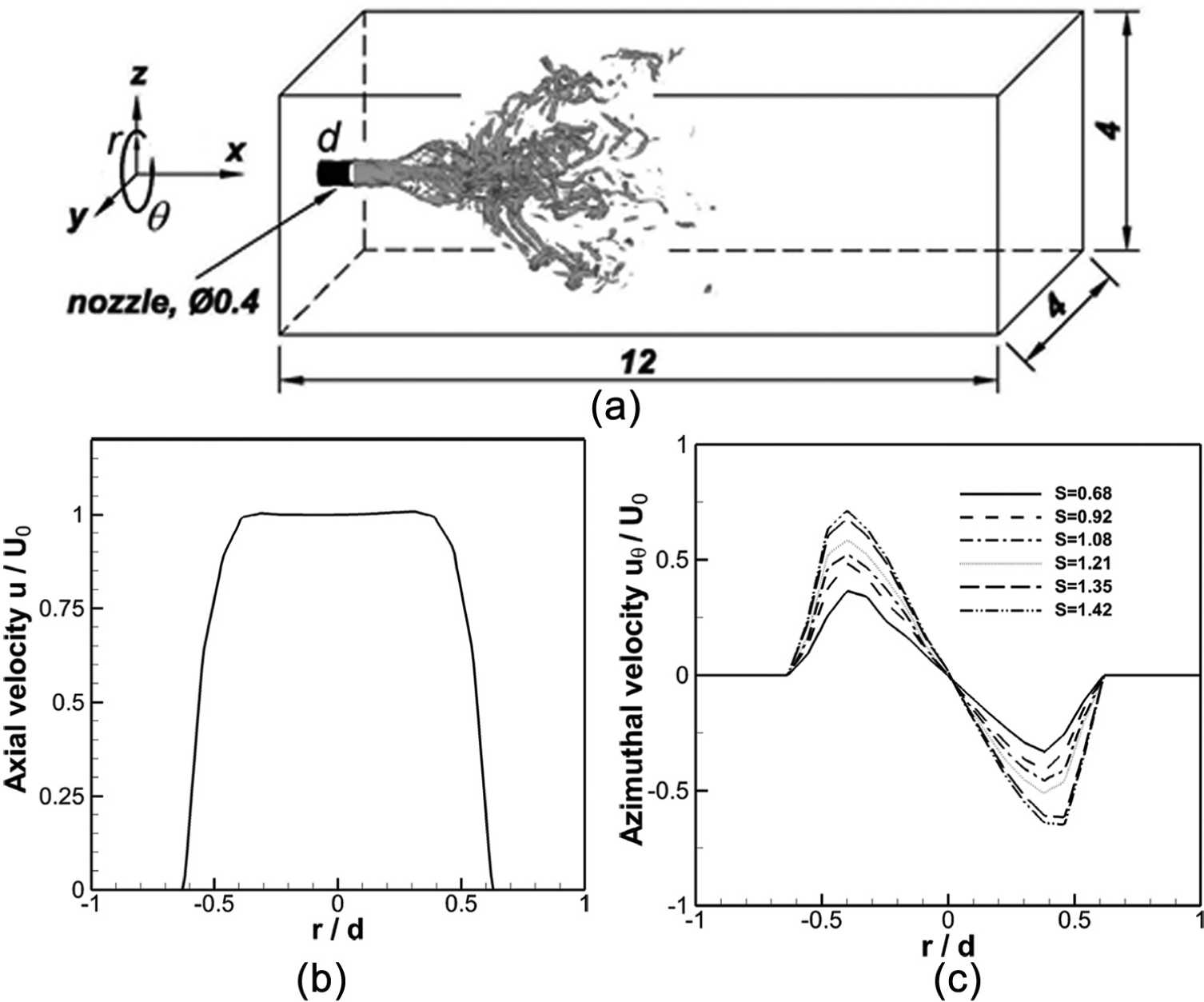
(a) The flow configuration, (b) axial inflow velocity, and (c) azimuthal inflow velocity for different levels of swirl.

Table 1.

Parameters used in the numerical simulation.

Scale of jet diameter d (mm)	0.4
Scales of the flow domain (X, Y, Z)	30d × 12d × 10d
Grid number Nx × Ny × Nz (–)	384 × 128 × 128
Mean inlet axial velocity U0 (–)	1.0
Reynolds number Re	606; 3000
Swirl number S	0.68, 0.92, 1.08, 1.35, and 1.42
Time step Δt (–)	0.005
Simulation time Ts (–)	100

To solve the governing equations (1) and (2), the finite volume method and the fractional-step projection technique¹⁴ are utilized. The central difference schemes are used for the spatial discretization, and an explicit low-storage, third-order Runge–Kutta scheme¹⁵ is used for temporal advancement. A direct fast elliptic solver is used to solve the Poisson equation. The validation for the current in-house code has been done by comparing the simulation results to the experiments in an early study.¹⁶

Boundary and operating conditions

As shown in Figure 1(b) and (c), the modeled profiles of the inlet velocities based on Billant et al.,⁸ that is, the axial and azimuthal velocities for different swirl numbers, respectively, are given. The velocities on the walls of the flow domain are set 0, except the outflow area where the non-reflecting boundary condition is applied.¹⁷

The swirl number S and the Reynolds number Re are the two important parameters. The swirl number is defined as the ratio of the maximum azimuthal velocity to the axial velocities here,⁸ which is

S = \frac{2 w_{\max}}{u_{a}}

(3)

where w_max and u_a are the azimuthal and axial inflow velocities, respectively. In this study, several levels of swirl are simulated, and the swirl numbers are included in Table 1.

For the spatial resolution requirement of direct numerical simulation, the vortex motion of the order of Kolmogorov length scales η = (ν³/ε)^1/4 is required to be captured.¹⁸ In the present simulation, 384×128× 128 mesh grids are used for spatial discretization. Under this condition, the mesh spacing is about 1.15η, which is of the order the Kolmogorov length scale. It has already been validated in a previous study at a low Reynolds number.¹⁶ Additionally, a moderate Reynolds number (Re = 3000) is also simulated. Although the mesh spacing is estimated about Δ≈ 3η,¹⁹ which is a bit larger than the Kolmogorov scale, they are still of the same order. Thus, the spatial resolution for direct numerical simulation is guaranteed, although not strictly. With this consideration, we used Re = 3000 in this study.

Simulation results

Structure of vortex cores

First, it is necessary to show the structure of vortex cores in swirling jets. The λ₂ definition is used to characterize vortex core in this section, which is the second eigenvalue (λ₁ < λ₂ < λ₃) of the symmetric tensor $S^{2} + Ω^{2}$ , where S and Ω are the symmetric and antisymmetric parts of the velocity gradient tensor, respectively.²⁰

Figure 2(a) and (c) illustrates the structures of vortex cores for S = 0.68 and 1.35 at Reynolds number Re = 606, respectively. Figure 2(b) and (d) shows the flux of radial velocities, through the cylindrical surface of r = d/2 from the jet axis for S = 0.68 and 1.35, respectively, which are used to indicate the corresponding vortex structures on the cylindrical surface. The conditions of S = 0.68 and 1.35 are categorized as the low level and the critical levels of swirl, respectively.⁸ It is observed from Figure 2(a) that helical vortex cores are formed symmetrically for the low swirl level of S = 0.68, that is, a cylindrical-helix pattern of four primary strong vortex core branches and four secondary weak helical vortex core branches encircling the jet axis (Figure 2(b)). The primary vortex cores are of a regular multi-cylindrical-helix configuration, whereas the secondary helical cores are so weak that they vanish in the downstream region (Figure 2(b)). In contrast, the VB takes place for the critical swirl level of S = 1.35, where stagnant fluids stay in the bubble VB (Figure 2(c), with zero velocity flux in the bubble VB region). In the downstream, the central vortex cores become spiral, rotating around the jet axis. It is so-called the processing of vortex cores (PVCs; Figure 2(d)). Moreover, the four primary helical vortex cores are broken down into more strongly spiral patterns, gradually divergent with respect to the jet axis, and vanish in the downstream due to the increased attenuation of helical motion.

Figure 2.

The three-dimensional structure of λ₂-vortex cores for (a) S = 0.68 and (c) S = 1.35 and flux of radial velocities through the cylindrical surface of r = d/2 for (b) S = 0.68 and (d) S = 1.35, respectively, at Reynolds number Re = 606.

In addition, when the level of swirl is supercritical (Figure 3(a), S = 1.42), a pattern of radiant processing vortex cores (RPVCs) is established (as sketched in Figure 3(b)). The primary helical vortex cores are generated from an upstream bubble. Due to viscous dissipation, the vortices are quickly attenuated in the downstream region. The helical vortex cores are kinked intensively because of the complicated flow pattern and interaction between vortex cores (Figure 3(a)). Moreover, it is necessary to mention that this kind of radiant pattern of processing vortex core has also been visualized in the experiments,⁸ where the cone type of VB is observed. In fact, the observation in the experiment is the projection of the RPVC onto the diagonal meridional plane.

Figure 3.

The λ₂-vortex cores for (a) S = 1.42 and (b) the corresponding sketch of the vortex structure at Re = 3000.

Velocity fields

To study the flow fields, Figure 4 shows the fields of mean fluid velocity in the near-field region. Figure 4(a)–(f) shows the axial variation in mean azimuthal velocity u_θ for S = 1.08 and Re = 3000 between x = 0.75d and x = 2.25d from the jet inlet. It is observed that small vortices are generated continuously from the inner rotating core. First, four vortices are generated due to the shearing effects and attached to the central core (Figure 4(a)). When these vortices are detached from the central core, new vortices are generated and attached then (Figure 4(b)). By repeating this procedure, the vortex core is processing downstream. Old vortices are detached from the central core into the periphery and become weakened, and new vortices are generated and attached to the central core (Figure 4(c)–(e)). Through the “detach–attach” cycle, new vortices are continuously originated until the central rotating core becomes so weak that it cannot maintain this cycle of vortex generation (Figure 4(f)). The “attach–detach” cycle indicates the general approach of vortex generation.

Figure 4.

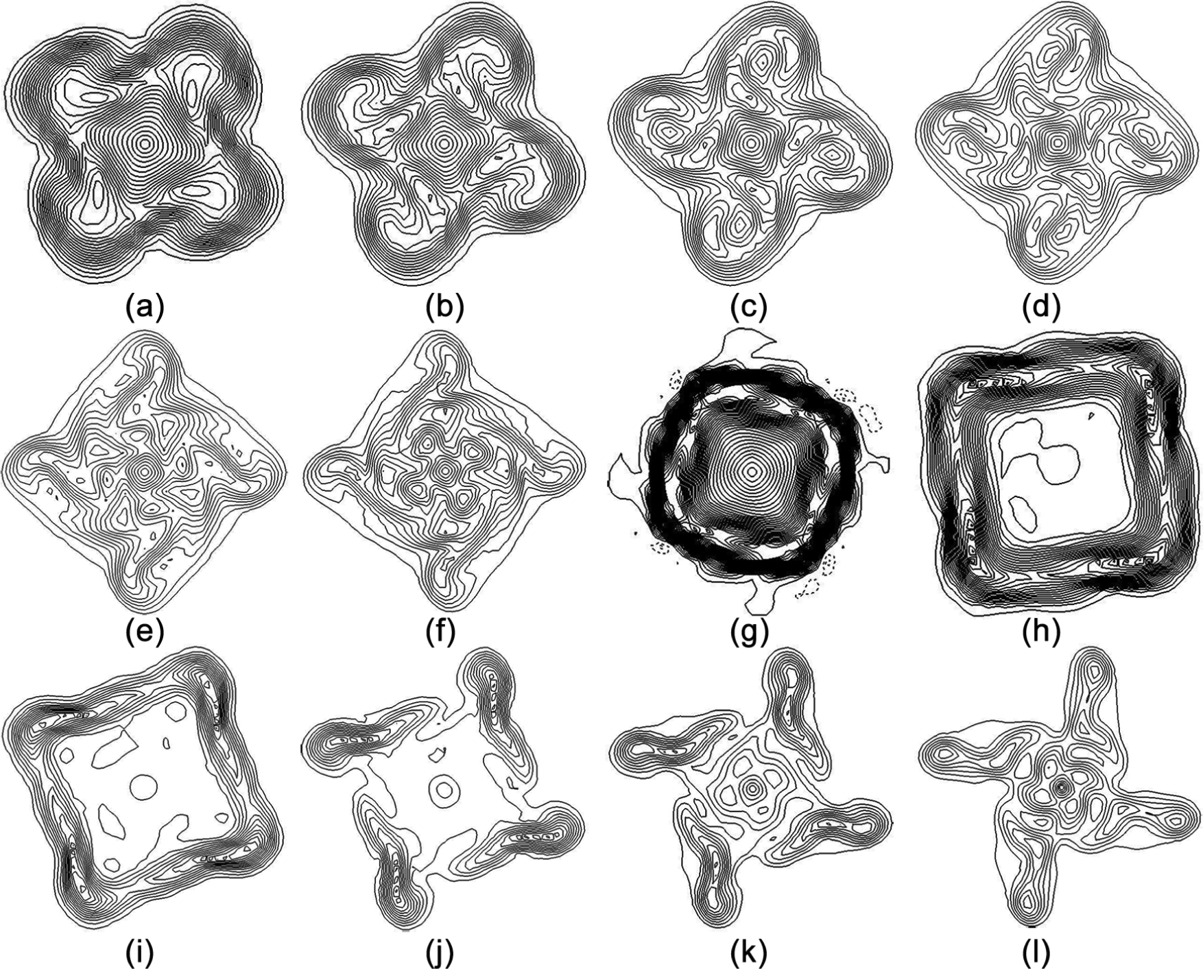
The axial variation in the mean azimuthal velocity u_θ for S = 1.08 ((a–f): x/d = 0.75–2.25 to the jet exit) and S = 1.35 ((g–l): x/d = 0–2.0 to the jet exit) in near-field region at Re = 3000.

Figure 4(h)–(l) corresponds to the azimuthal velocity u_θ for S = 1.35 and Re = 3000 from x = 0d to 2.25d. Unlike Figure 4(a)–(f) for S = 1.08, the central core vanishes, and the concentric rings of the azimuthal velocity occur (Figure 4(g)) due to the super centrifugal effect of rotation. In fact, these rings are the shearing layers. The inner rings correspond to the region with $\nabla_{r} u_{θ} > 0$ , and the outer rings correspond to the region with $\nabla_{r} u_{θ} < 0$ . A region of stagnant fluid ( $\nabla_{r} u_{θ} = 0$ ), that is, the location of the bubble VB (Figure 4(h) and (j)), is enclosed within the inner rings. At the tail of the bubble, the vortices are contracted, reproducing the central rotating core (Figure 4(k)). Then, the vortices are attached from the rings (Figure 4(l)), following the same mechanism of “detach–attach” cycle as before, although the strength of rotation is considerably attenuated due to the bubble VB.

In conclusion, the vortices are generated from the central rotating core through a “detach–attach” cycle for the low swirl level. The vortex cores are of a regular multi-cylindrical-helix configuration accordingly. Contrarily, the central rotating core is separated on the stagnation point into the concentric rotating rings due to the supercritical centrifugal effect for the high swirl level, and the fluid within the rotating rings is stagnant. In the downstream of the bubble, the vortices are contracted due to attenuation of the centrifugal effect. Then, the central rotating core appears again.

Microscopic rotating motion

In general, the velocity gradient tensor $\nabla V$ can be reformulated as

\nabla V = S + Ω = \frac{1}{2} (\nabla V + {(\nabla V)}^{T}) + \frac{1}{2} (\nabla V - {(\nabla V)}^{T})

(4)

where the symmetrical part $S = 1 / 2 (\nabla V + {(\nabla V)}^{T})$ denotes the deformation motion of fluids, whereas the antisymmetrical part $Ω = 1 / 2 (\nabla V - {(\nabla V)}^{T})$ denotes the microscopic rotation motion of fluids.

In swirling jets, the velocity gradient exists mostly between the azimuthal layers as well as the axial layers. It is common to use the probability density function (PDF) of vorticity components $ω_{i} = (\partial u_{k} / \partial x_{j}) - (\partial u_{j} / \partial u_{k}) (i, j, k = x, y, z)$ to evaluate the effect of microscopic rotating motion. Recalling that any instantaneous fluid motion is divided into the time-averaged and the fluctuation components, that is, $u_{i} = {\bar{u}}_{i} + u'_{i}$ , the vorticity component can be divided into two parts correspondingly, that is, the mean component ${\bar{ω}}_{i} = (\partial {\bar{u}}_{k} / \partial x_{j}) - (\partial {\bar{u}}_{j} / \partial u_{k})$ and the fluctuation component $ω'_{i} = (\partial u'_{k} / \partial x_{j}) - (\partial u'_{j} / \partial u_{k})$ . The mean component ${\bar{ω}}_{i}$ represents the microscopic rotating effects with regard to the mean fluid motions, whereas the fluctuation component $ω_{i}^{'}$ indicates the microscopic rotating effects with regard to the turbulent fluctuations.

For example, the PDFs of the mean and fluctuation components of the axial component of vorticity ω_x, which indicate the microscopic rotating effects in the cross-sectional plane, are shown in Figure 5. For comparison, the ω_x is normalized by the root mean square (r.m.s.) value of it. For clarity, these variables are formulated as

\begin{matrix} {〈 {\bar{ω}}_{x} 〉}_{r . m . s .} = {(\frac{1}{Σ} \int_{Σ} {(ω_{x} (r) - 〈 {\bar{ω}}_{x} 〉)}^{2} d r)}^{1 / 2}, \\ 〈 {\bar{ω}}_{x} 〉 = \frac{1}{Σ} \int_{Σ} ω_{x} (r) d r \end{matrix}

(5)

\begin{matrix} {〈 ω_{x}^{'} 〉}_{r . m . s .} = {(\frac{1}{Σ} \int_{Σ} {(ω_{x}^{'} (r) - 〈 ω_{x}^{'} 〉)}^{2} d r)}^{1 / 2}, \\ 〈 ω_{x}^{'} 〉 = \frac{1}{Σ} \int_{Σ} ω_{x}^{'} (r) d r \end{matrix}

(6)

where ${\bar{ω}}_{x} = {\bar{ω}}_{x} (r) = ((1 / T_{s}) \int_{T_{s}} ω_{x} (r, t) dt), ω_{x}^{'} = ω' (r) = {((1 / T_{s}) \int_{T_{s}} {(ω_{x} (r, t) - {\bar{ω}}_{x})}^{2} dt)}^{1 / 2})$ are the mean component and fluctuation components, respectively. T is the simulation time, and $Σ$ is the simulation domain. The operator “ $\bar{•}$ “ represents the temporal-average operator, whereas the operator “ $〈 • 〉$ ” represents the spatial-average operator.

Figure 5.

The probability density function of (a) the normalized mean vorticity component ${\bar{ω}}_{x} / {〈 {\bar{ω}}_{x} 〉}_{r . m . s .}$ and (b) the normalized fluctuation of vorticity component $ω'_{x} / {〈 ω'_{x} 〉}_{r . m . s .}$ .

Then, as shown in Figure 5(a), the normalized mean components of vorticity ${\bar{ω}}_{x}$ for different swirl levels are not clearly different from each other. By detailed comparison, it is observed that the PDFs of large swirl numbers (S = 1.35 and 1.42) are generally larger in the tails than that of small swirl numbers (S = 0.68 and 0.92). Remember that the effect of swirl level plays a predominate role in determination of the structure of vortex cores in swirling jets (Figures 2 –4). However, it changes few, if yes, of the PDFs of the mean microscopic rotating motion.

In contrast, it is observed from Figure 5(b) that the PDFs of the microscopic rotating effects with regard to the turbulent fluctuations $ω_{x}^{'}$ are closely related to the levels of swirls. The larger swirl numbers lead to the larger tails of the PDFs, and vice versa. As well known, the large tails of the PDFs indicate the intermittent characteristics. Thus, it is interesting to find that a large swirl level indicates the greater intermittent distribution of the microscopic rotating effect with respect to the turbulent fluctuation motions in the swirling jets. On the opposite side, a low swirl level indicates the less intermittent distribution of the microscopic rotating effect with respect to the turbulent fluctuation motion. Moreover, the results also show that the microscopic rotating motion with respect to turbulent motions is more sensitive upon the swirl levels than that for the mean motions.

The microscopic rotating effects with respect to the fluctuation motions are more significant than that of the mean flow fields due to the complicated characteristics of turbulence. Thus, the augmented intermittency of spatial distribution of the microscopic rotating effects with the increased swirl level indicates the strong dependency of intrinsic feature of anisotropic turbulence upon the swirl levels.

Macroscopic rotating motion

As the swirling flow is mainly characterized by the superposition of the macroscopic rotating motion upon the axial motion, it is necessary to evaluate the macroscopic rotating effects by the angular momentum with respect to the jet axis. Similarly, we used the PDFs of the angular momentum with respect to jet axis. In general, the total angular momentum is defined as the cross product of r(x,y,z) and u = (u,v,w): $Ω = r \times u$ . With respect to the jet axis, the x component of the total angular momentum is used in this study. Thus, the mean angular momentum ${\bar{Ω}}_{x}$ and the fluctuation of angular momentum $Ω_{x}^{'}$ are appropriately formulated, respectively, as

{\bar{Ω}}_{x} = {(r \times \bar{u})}_{x} = (r \times \bar{u}) • x^{0}

(7)

Ω'_{x} = {(r \times u')}_{x} = (r \times u') • x^{0}

(8)

where x⁰ is the unit vector in the axial direction.

The PDFs of the mean and fluctuation components of the macroscopic rotating motion are shown in Figure 6(a) and (b), respectively. In Figure 6(a), the normalized PDFs of the mean macroscopic rotating motion ${\bar{Ω}}_{x}$ are asymmetrical in the x-axis because the given macroscopic rotating motion is anticlockwise with respect to the jet axis. It is seen that the PDFs are larger for swirl numbers S = 1.35 and 1.42 than those for S = 0.68 and 0.92. Thus, the mean angular momentum increases with the levels of swirl. It is reasonable and reflects the definition of swirl level by equation (3).

Figure 6.

The probability density function of (a) the normalized mean angular moment ${\bar{Ω}}_{x} / {〈 {\bar{Ω}}_{x} 〉}_{r . m . s .}$ and (b) the normalized fluctuation of angular moment $Ω'_{x} / {〈 Ω'_{x} 〉}_{r . m . s .}$ .

However, more interestingly, the above conclusion is not true for the fluctuation of the angular momentum, that is, a large swirl level does not indicate the greater fluctuation of the macroscopic rotating motion. As seen in Figure 6(b), the PDFs of the fluctuation of angular momentum $Ω'_{x}$ are of relatively both low values for the largest swirl numbers (e.g. S = 1.42) and the smallest swirl numbers (e.g. S = 0.68). On the contrary, the largest PDFs of $Ω'_{x}$ occur at moderate swirl levels (S = 1.08). The reason is considered to be closely related to the pattern of vortex cores. It seems that the fluctuation of the macroscopic rotating motion becomes augmented with the increase in the swirl levels when the swirl level is below the critical swirl level (S < S_c = 1.35). Then, the fluctuation of the macroscopic rotating motion is attenuated for the supercritical swirl level (S = 1.42 ≥ S_c) due to the formation of stagnant fluids within the bubble VB (Figure 4(h)–(j)). With the stagnant fluid, the fluctuation of the macroscopic rotating motion is considerably dissipated and attenuated. It can neither maintain nor augment the turbulent rotation motion as before. However, in that case, the PDFs with respect to the fluctuation of macroscopic rotating motion are still large than the case for low swirl levels (S = 0.68 and 0.92).

The difference between the PDFs of the macroscopic and microscopic rotating motions with respect to the turbulent fluctuations indicates an important feature of anisotropic turbulence. The microscopic rotating effect is related to the local characteristics of turbulent fluctuation whereas the macroscopic rotating effect is related to the global motion characteristics. The local intermittency is clearly dependent on the swirl levels whereas the global distribution of rotation fluctuation is largely influenced by the structure of vortex cores.

Conclusion

The main findings of this study are briefly concluded in the following:

The structure of vortex cores in swirling jets is divided into two categories according to the levels of swirl, that is, the multi-cylindrical-helix pattern for the low swirl and the VB followed by the RPVC pattern for the high swirl level.

The microscopic rotating effects with respect to the mean and fluctuation components of turbulence are evaluated. A large swirl level leads to an augmented intermittency of the microscopic rotating effect with respect to the fluctuation motion and vice versa. But it is not evident for the microscopic rotating effect of the mean flow to depend on the swirl levels.

The fluctuation of the macroscopic rotating motion is closely related to the global pattern of vortex cores. The maximum fluctuation of the macroscopic rotating motion occurs at moderate swirl levels. It is true that the increase in swirl can lead to the increase in rotation fluctuation. But the formation of bubble VB and the stagnant fluid can counteract the increase in the fluctuation of rotation effects as well.

Footnotes

Academic Editor: Sandra Velarde Suarez

Declaration of conflicting interests

The authors declare that there is no conflict of interest.

Funding

This study was supported by the National Natural Science Foundation of China (51106180) and the Foundation for the Author of National Excellent Doctoral Dissertation of P.R. China (FANEDD, grant no. 201438).

References

Gupta

Lilley

Syred

. Swirl flows. New York: Abacus, 1984.

Saffman

. Vortex dynamics. Cambridge: Cambridge University Press, 1992.

Syred

Beer

. Combustion in swirling flows: a review. Combust Flame 1974; 23: 143–201.

Lambourne

Bryer

. The bursting of leading-edge vortices: some observations and discussion of the phenomenon. ARC R&M No. 3282. London: Her Majesty’s Stationery Office, 1961.

Sarpkaya

. On stationary and travelling vortex breakdowns. J Fluid Mech 1971; 45: 545–559.

Sarpkaya

. Turbulent vortex breakdown. Phys Fluid 1995; 7: 2301–2303.

Khoo

Yeo

Lim

. Vortex breakdown in an unconfined vortical flow. Exp Therm Fluid Sci 1997; 14: 131–148.

Billant

Chomaz

Huerre

. Experimental study of vortex breakdown in swirling jets. J Fluid Mech 1998; 376: 183–219.

Faler

Leibovich

. Disrupted states of vortex flow and vortex breakdown. Phys Fluid 1977; 20: 1385–1400.

10.

Mcllwain

Pollard

. Large eddy simulation of the effects of mild swirl on the near field of a round free jet. Phys Fluid 2002; 14: 653–661.

11.

Wang

Bai

Wessman

. Large eddy simulation and experimental studies of a confined turbulent swirling flow. Phys Fluid 2004; 16: 3306–3324.

12.

Serre

Bontonx

. Three-dimensional swirling flow with a processing vortex breakdown in a rotor-stator cylinder. Phys Fluid 2001; 13: 3500–3503.

13.

Ruith

Chen

Meiburg

. Three-dimensional vortex breakdown in swirling jets and wakes: direct numerical simulation. J Fluid Mech 2003; 486: 331–378.

14.

Chorin

. Numerical solution of the Navier-Stokes equations. Math Comput 1968; 22: 745–762.

15.

Williamson

. Low-storage Runge-Kutta schemes. J Comput Phys 1980; 35: 48–56.

16.

Gui

Fan

Cen

. A direct numerical simulation study of coherent oscillation effects of swirling flows. Fuel 2010; 89: 3926–3933.

17.

Orlanski

. A simple boundary condition for unbounded hyperbolic flow. J Comput Phys 1976; 21: 251–269.

18.

Moin

Mahesh

. Direct numerical simulation: a tool in turbulence research. Annu Rev Fluid Mech 1998; 30: 539–578.

19.

Gui

Fan