
Abstract
For the solution of geometrically nonlinear analysis of plates and shells, the formulation of a nonlinear nine-node refined first-order shear deformable element-based Lagrangian shell element is presented. Natural co-ordinate-based higher order transverse shear strains are used in present shell element. Using the assumed natural strain method with proper interpolation functions, the present shell element generates neither membrane nor shear locking behavior even when full integration is used in the formulation. Furthermore, a refined first-order shear deformation theory for thin and thick shells, which results in parabolic through-thickness distribution of the transverse shear strains from the formulation based on the third-order shear deformation theory, is proposed. This formulation eliminates the need for shear correction factors in the first-order theory. To avoid difficulties resulting from large increments of the rotations, a scheme of attached reference system is used for the expression of rotations of shell normal. Numerical examples demonstrate that the present element behaves reasonably satisfactorily either for the linear or for geometrically nonlinear analysis of thin and thick plates and shells with large displacement but small strain. Especially, the nonlinear results of slit annular plates with various loads provided the benchmark to test the accuracy of related numerical solutions.
Keywords
Introduction
Due to their attractive properties, shells are used in a variety of engineering structures, such as arch dams, dome structures, pressure-vessels, ship hulls, and aircraft fuel-ages. In order to fully utilize their special structural features, efficient and reliable analysis tools are needed for the prediction of their structural behaviors. Now the finite element method is a major tool for numerical analysis of shell structures because of their intrinsic complexities. Over the past 50 years, many shell elements have been developed. Many shell element formulations have been based on the so-called degenerate models introduced by Ahmad et al. 1 While such elements are capable of dealing with thick plate and shell problems, their performance deteriorates rapidly as the element thickness becomes thin, which is called shear locking. In order to overcome the shear locking problems, Huang and Hinton 2 developed a nine-node assumed strain shell element using the enhanced interpolation of the transverse shear strains in the natural coordinate system. The assumed natural strain method can be traced to MacNeal 3 and Dvorkin and Bathe. 4 Many finite elements employing the assumed strain method were then reported by other research groups independently.5,6 Furthermore, some applications of the assumed strain method have been made in the field of large deformation analysis. In particular, assumed strain has been expressed in the form of natural strain because of its simplicity. In order to avoid shear locking in the plate and shell elements, Nguyen-Xuan et al. 7 and Nguyen-Thanh et al. 8 proposed a smoothed finite element, respectively. Recent years, Rodrigues et al. 9 developed smoothed finite element for analysis of composite plates. In this study, the element-based Lagrangian formulation (ELF) by Kanok-Nukulchai and Wong 10 is used and it makes implementation simpler and easier than the traditional Lagrangian formulations, especially when the assumed natural strain method is involved.
Zhang and Kim 11 developed a refined non-conforming triangular plate/shell element for linear and geometrically nonlinear analysis of plates and shells. The drilling rotation constraint (RC) equation was used in the work 12 with the Hu–Washizu (HW) functional. Various forms of governing functionals modified by the RC are presented in Wisniewski. 12 Defining the assumed representations of stress and strain in the four-node HW elements, Wisniewski and Turska13,14 used the skew coordinates instead of the natural ones. Firl and Bletzinger 15 studied the shape optimization of thin-walled structures. Shin and Lee 16 proposed a three-node triangular flat shell element based on the assumed natural deviatoric strain with drilling degrees of freedom. Also, a three-dimensional (3D) nonlinear analysis using a resultant eight-node solid element is presented by Kim et al. 17 and Ahmed et al. 18
The first-order shear deformable shell elements are usually capable of also producing good results for the in-plane strain and stress distribution, but their formulation results in constant transverse shear strains as opposed to the realistic parabolic distribution. As a result, the traction conditions at the shell surfaces are violated. They also require shear correction coefficients to correct the corresponding strain energy terms and these coefficients are problem dependent and are not always easy to determine. Numerous efforts have been made to overcome this disadvantage of the first-order formulation, most of which result in a higher order shear deformation theory.19–21 The equilibrium approach suggested by Rolfes and Rohwer 22 was used for the calculation of the transverse shear stiffness in Kim at al. 5 Tanov and Tabiei 23 presented an approach for treating the transverse shear strains and stresses in homogeneous shells resulting in parabolic distribution for both strains and stresses and, therefore, it eliminates the need of any shear correction factors. It requires only minor changes in the first-order shear deformation formulation. The implementation in shell element was shown to be quite simple and straightforward in Han et al.24,25 and Jung and Han. 26 The proposed nine-node shell element will consider parabolic through-thickness distribution of the refined transverse shear stresses and strains based on simple corrections to the first-order theory proposed by Han et al. 24
In large deformation analysis, two steps are involved in obtaining the linearized nonlinear equations. First, nonlinear equations of the structural system have to be derived via Lagrangian formulations. Second, the linearization of the nonlinear equations is required to solve nonlinear equations by an iterative method such as the arc-length control method. So far, traditional Lagrangian formulations, which are total Lagrangian formulation (TLF) and updated Lagrangian formulation (ULF), have been extensively used for deriving the nonlinear equation. Unlike two formulations of the above, new Lagrangian formulation was introduced and it was referred to as the ELF since the fundamental element serves as a deformation reference in ELF. 7 It means that all equations governing a deformed body can be expressed with respect to natural coordinate systems. For the large deformation analysis of shells, the expression of rotations plays an important role to define a proper position of shell normal vector. In this study, three successive finite rotations are introduced since the drilling degree of freedom is used for the present shell element.27,28
The objective of this research work is the development of a finite element for geometrically nonlinear shells with emphasis on the generality, robustness, and efficiency. The proposed element is a nine-node Lagrangian-type degenerated shell element. The element is based on the refined first-order shear deformation theory, and therefore is independent of the need of any shear correction factors. In the element formulation, an appropriate strain interpolation is employed to avoid both the shear and the membrane locking phenomena. Also, a suitable scheme is pursued for the expression of the rotational degrees of freedom so that the limitation on magnitude of the rotational increment in each load step can be removed. A full Gauss integration scheme is applied for the evaluation of the torsional stiffness.
The proposed formulation is computationally efficient and the test results showed good agreement. More specifically, the numerical examples of annular plate presented herein show good validity, efficiency, and accuracy for the developed nonlinear shell element.
Geometry and kinematics of the shell element
In Figure 1, the geometry of a nine-noded shell element with 6 degrees of freedom is illustrated.

Geometry of nine-node shell element with 6 degrees of freedom.
The position vector and the displacement vector of the refined first-order shear deformation theory of nine-node shells can be simplified into 24

where
Using the tensor transformation relationship of Green strain tensor and the natural strain, the transverse natural shear strains can obtain 24

When the effective transverse shear energy (

where

The refined first-order shear deformation theory can then be presented as a function of

The limitation of modified first-order shear deformation theory 24 is overcome using equation (5) for the correct analysis of thin and thick shells. Equation (5) is different from the usual natural strain relations of first-order shear deformation theory and the results in parabolic through-thickness distribution for the transverse shear strains.
The incremental displacement field within the element can be expressed as
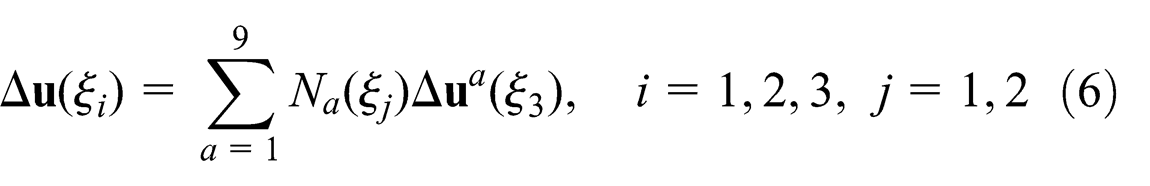
where
The shell element displays resultant membrane forces, moments, and transverse shear forces obtained by integration of stresses through the thickness using the equivalent constitutive equations


where
Assumed natural strains
Ma and Kanok-Nukulchai 27 suggested the procedure for classifying the optimal locations of the sampling points to avoid locking phenomena. It was utilized by Han et al. 24 The membrane and transverse shear strain fields are interpolated with the following sampling points in Figure 2.

Sampling points for assumed strains of (a) membrane normal and transverse shear and (b) membrane shear.
Static equilibrium equation
The static equilibrium equation can be derived as
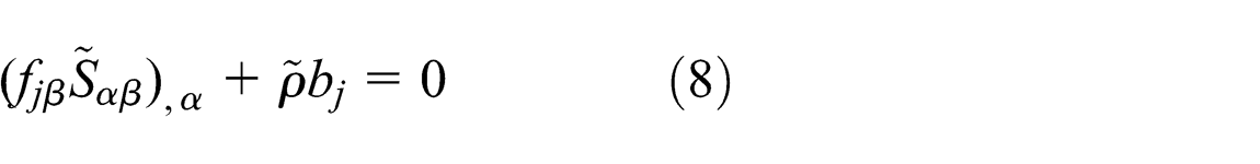
where

and

in which
The weak form of the static problem can be constructed by Galerkin’s weighted residual method as

where

The weight field of Galerkin’s method has the same function space as the displacement field, so the weight field can be expressed as

where
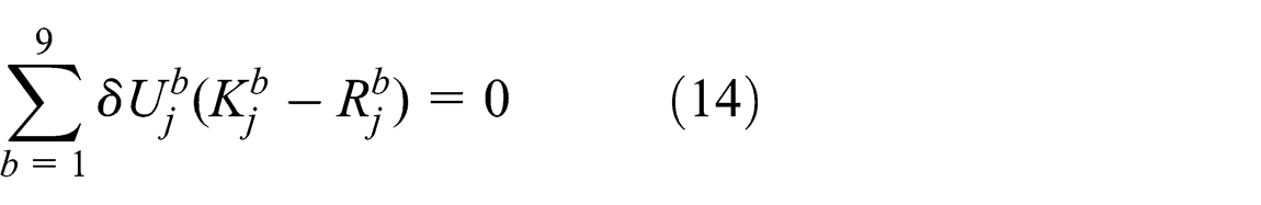
in which
Since

The drilling degree of freedom will be linked to the in-plane twisting mode of the mid-surface by a penalty functional. 29
Tangent stiffness and arc-length control method
To solve the nonlinear equation by the Newton–Raphson method, the linearization is required, and the result is the element tangent stiffness matrix in the form
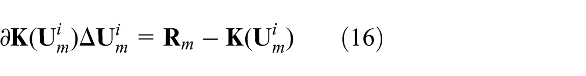
where

In order to trace the full path of load–displacement, it is necessary to use the arc-length control method, since the postbuckling study involves a highly distorted load–displacement path. With consideration of the incremental load step, equation (15) can be rewritten in the following form which has (n + 1) unknowns

where

where
Linearization of equation (18) and the constraint equation
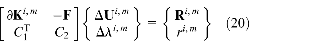
where
Numerical examples
Several numerical examples are solved to test the performance of the shell element in geometrically nonlinear applications. Examples included isotropic plates to check some crucial features and shells for the comparisons and further developments. Before the various sections, nonlinear examples of hemispherical shells are treated. First, nonlinear isotropic hemispherical shell with
Nonlinear analysis of hemispherical shell
The problem configuration of hemispherical shell with an

Definition of loading points and initial configuration of
Load–deflection curves for
Initial configuration and deformed configuration of
The next example considered is the full pinched hemispherical shell under two inward and two outward opposite forces (Figure 6). In this case, we consider a full hemisphere with no hole. The radial displacement at points A and B is monitored in Figure 7. Comparisons of the present results with those of Arciniega and Reddy
33
are in close agreement, but the reference results are slightly stiffer. Arciniega and Reddy
33
used a regular mesh of

Definition of loading points and initial configuration of hemispherical shell.

Load–deflection curves for a full hemispherical shell.

Initial configuration and deformed configuration of full hemispherical shell: (a) initial configuration and (b) deformed configuration.
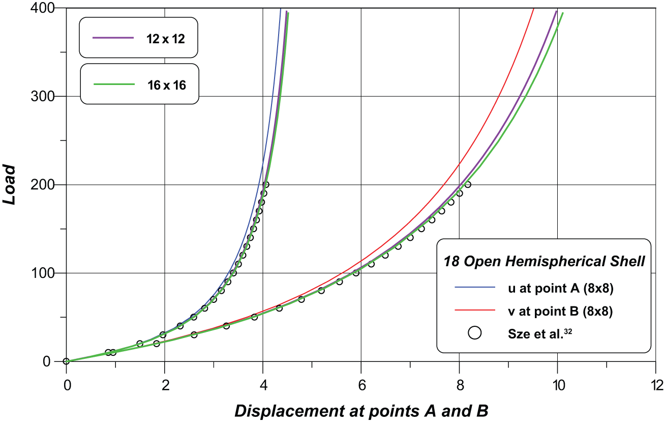
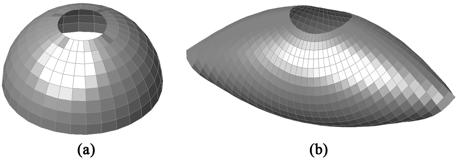
The third example considered is the hemispherical shell with an 18° circular cutout at its pole. In the first example, the thickness
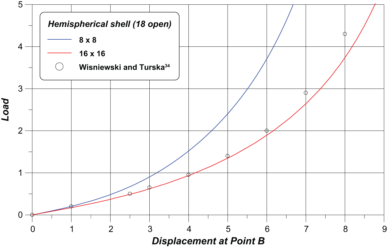
Load–deflection curves for
Nonlinear analysis of twisted beam
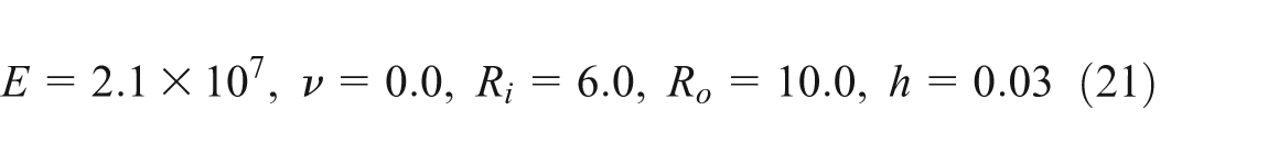
The initial geometry of the beam is twisted, but the initial strain is equal to 0. The beam is clamped at one end and loaded by a unit force at the other. The force is applied either along the y-axis (in-plane) or along the x-axis (out-of-plane), see Figure 10. Here, we provide the results for the latter case only. The data are as follows:
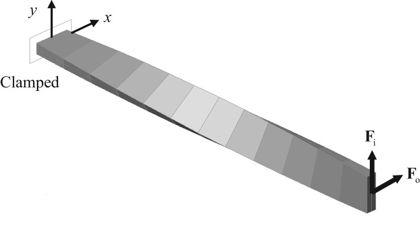
Definition of loading points and initial configuration of twisted beam.
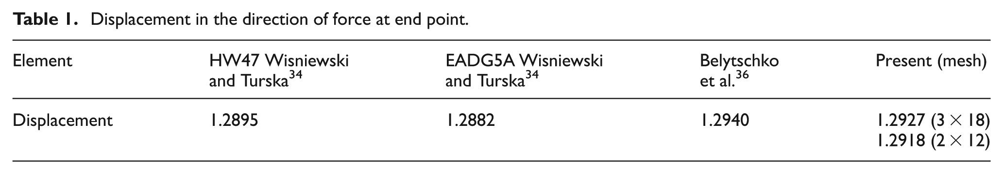
Displacement in the direction of force at end point.
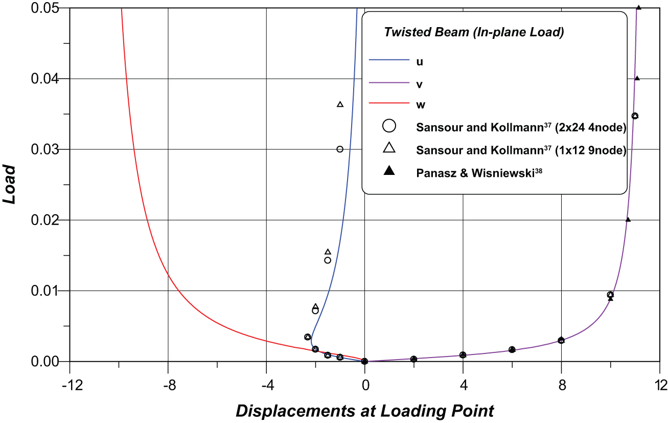
Load–deflection curves for a twisted beam under in-plane load.

Load–deflection curves for a twisted beam under out-of-plane load.
Nonlinear analysis of C-shape narrow plate
The C-shape narrow plate problems are shown in Figure 13 with sequence of deformed configuration with tip bending moment. The total length of C-shape narrow plate is

Sequence of deformed finite element meshes corresponding to the increasing loads of C-shape narrow plate. End B is fixed. End A is free with bending moment.
Nonlinear analysis of pinched cylinder of a clamped cylinder
Another well-known benchmark problem of finite deformation is the pinched cylindrical shell under a point load (Figure 14(a)). This problem has been investigated by Balah and Al-Ghamedy,
39
Sze et al.,
32
and Arciniega and Reddy.
33
The material properties are as follows: Young’s modulus

Problem definition and a deformed configuration of pinched cylinder with free edge: (a) initial configuration and (b) deformed configuration.

Load–deflection curve of clamped cylindrical shell under pinching point load.
Nonlinear analysis of slit annular plate
Annular plate under end out-of-plane shear force
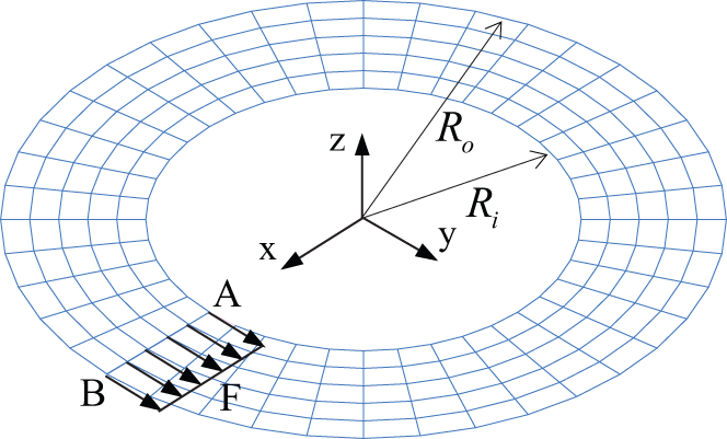
In order to validate the present shell element, a numerical example of annular plate under end shear force is solved. We examine an annular clamped plate subjected to a distributed transverse shear force (Figure 16). This beautiful benchmark problem was considered by Sansour and Kollmann 37 and Arciniega and Reddy, 33 among others, and Sze et al. 32 presented ABAQUS results for the problem. In particular, we use the ABAQUS results presented in a recent article of Sze et al. 32 for popular benchmark problems of nonlinear shell analysis (because of the tabulated data). The geometry and elastic material properties for the isotropic case are given by

Slit annular plate loaded with various end forces F.
for a maximum distributed force of

Load–deflection curves for the slit annular plate lifted by line force F.

Load–deflection curves for the slit annular plate lifted by line force F.

Deformed configuration of the slit annular plate (5 × 40 mesh) for F = 1.45.
Annular plate under end moment
We examine an annular clamped plate subjected to end loads (Figure 20). The load versus displacement curves for two characteristic points are depicted in Figure 21. Figure 22 shows the deformed configuration of the isotropic annular plate for load level

Slit annular plate loaded with various end forces F.

Load–deflection curves for the slit annular plate deformed by two point forces.
Deformed configuration of the slit annular plate (5 × 40 mesh) for F = 10.0.
Annular plate under end in-plane force (
)
We examine an annular clamped plate subjected to end loads (Figure 23). To activate the postbuckling equilibrium path we have to include a small perturbation in the system. Otherwise, only in-plane displacements in the plate will occur (which is called the fundamental equilibrium path beyond which the critical load will be unstable). For the secondary path, we assume that the annular plate is presented with an imperfect displacement of
Slit annular plate loaded with various end forces F.

Load–deflection curves for the slit annular plate lifted by line force F.

Deformed configuration of the slit annular plate (5 × 40 mesh) for F = 0.38.
Annular plate under end in-plane force (
)
We examine an annular clamped plate subjected to end loads (Figure 26). The load versus displacement curves for two characteristic points are depicted in Figure 27. Figure 28 shows the deformed configuration of the isotropic annular plate for load level

Slit annular plate loaded with various end forces F.

Load–deflection curves for the slit annular plate lifted by line force F.

Deformed configuration of the slit annular plate (5 × 40 mesh) for F = 0.55.
Annular plate under end in-plane shear force (
)
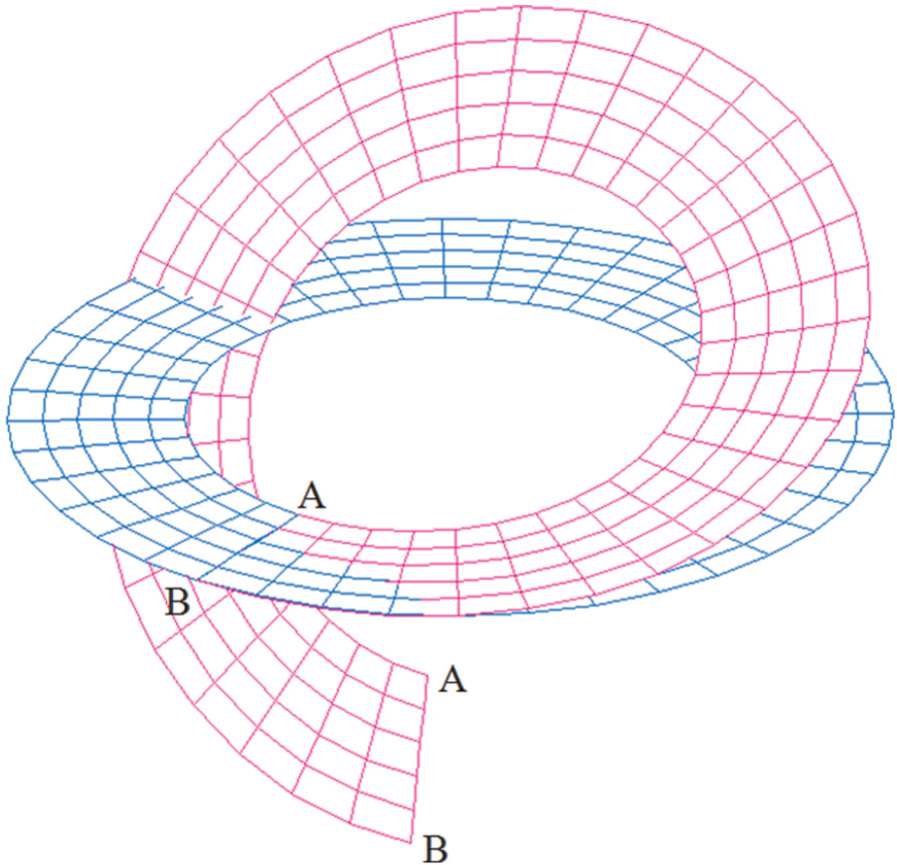
We examine an annular clamped plate subjected to end loads (Figure 29). The load versus displacement curves for two characteristic points are depicted in Figure 30. Figure 31 shows the deformed configuration of the isotropic annular plate for load level

Slit annular plate loaded with various end forces F.

Load–deflection curves for the slit annular plate lifted by line force F.

Deformed configuration of the slit annular plate (5 × 40 mesh) for F = 1.40.
Annular plate under end in-plane shear force (
)
We examine an annular clamped plate subjected to end loads (Figure 32). The load versus displacement curves for two characteristic points are depicted in Figure 33. Figure 34 shows the deformed configuration of the isotropic annular plate for load level

Slit annular plate loaded with various end forces F.

Load–deflection curves for the slit annular plate lifted by line force F.
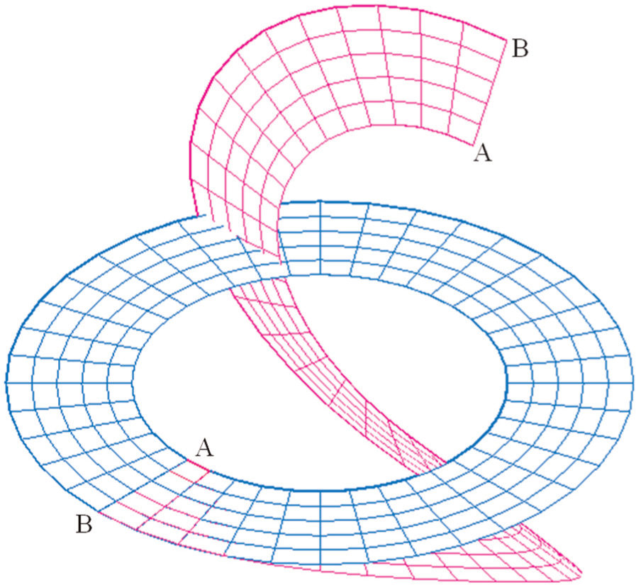
Deformed configuration of the slit annular plate (5 × 40 mesh) for F = 0.2875.
Nonlinear analysis of hinged shell
This is a widely used example for testing geometrically nonlinear shell elements. In this study, a quadrant of the shell is modeled with

Hinged cylindrical shell; curved edges are free, straight edges are hinged (P = 1000).
For the case of h = 12.7 mm, the average number of iterations is 5, and the curve of the central deflection versus load is given in Figure 36, showing the good correlation between the present solution and the reference solutions.

Load–deflection curves for the hinged shell (h = 12.7 mm).
For the case of h = 6.35 mm, the solution derived with

Load–deflection curves for the hinged shell (h = 6.35 mm).
In the third case of this analysis, even a further reduction in the panel thickness was presumed taking h = 3.175 mm, what resulted in a rather complicated shape of the equilibrium path. The curve of the central deflection versus load is given in Figure 38.
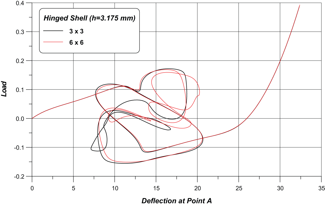
Load–deflection curves for the hinged shell (h = 3.175 mm).
Nonlinear analysis of pullout of an open-ended cylindrical shell
The example consists of a cylindrical shell with open ends, which is pulled by a pair of radial forces. The geometrical data and material properties are presented in Figure 39. The problem has been considered in Sansour and Kollmann, 37 Sze et al., 32 and Arciniega and Reddy, 33 among others. Owing to symmetry, one-eighth of the shell is modeled and a mesh with six elements along the circumferential direction and four elements along the longitudinal direction is adopted. Points A, B, C, and D are monitored in terms of radial displacement in Figure 40. The displacements for points A–D are compared with the results obtained by Sze et al. 32 It is noticed that the response of the shell has two different regions: the first is dominated by bending stiffness with large displacements; the second, at load level of P = 20,000, is characterized by a very stiff response of the shell. The deformed configuration under the load level of P = 40,000 is portrayed in Figure 41.
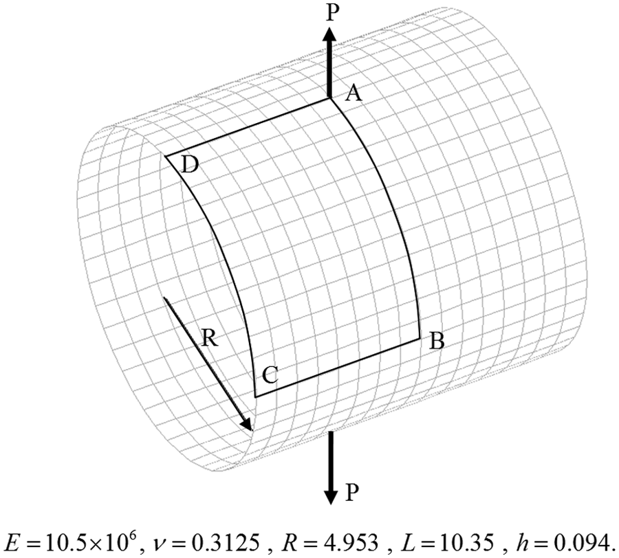
Open-end cylindrical shell subjected to radial pulling forces (P = 40,000).
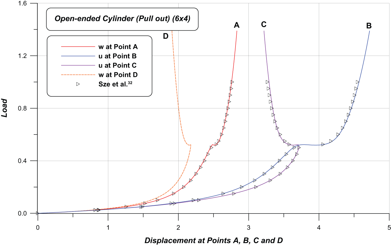
Load–deflection curves for the open-end cylindrical shell.

Deformed configuration of the cylindrical shell (6 × 4 mesh) for P = 40,000.
Nonlinear analysis of pinched cylindrical shell
The pinched cylindrical shell mounted on rigid end diaphragms is shown in Figure 42. The example consists of a cylindrical shell subjected to two radial opposite forces. The dimensions and the material properties for one-eighth of the shell are illustrated in Figure 42. Due to symmetry, one-eighth of the shell is modeled and the employed mesh for nine-node shell elements is
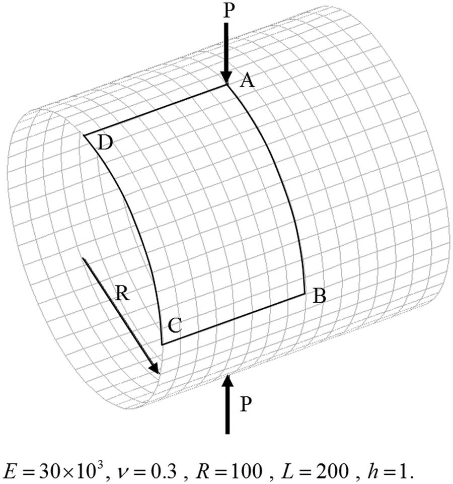
Pinched cylindrical shell mounted on rigid end diaphragms (P = 12,000).
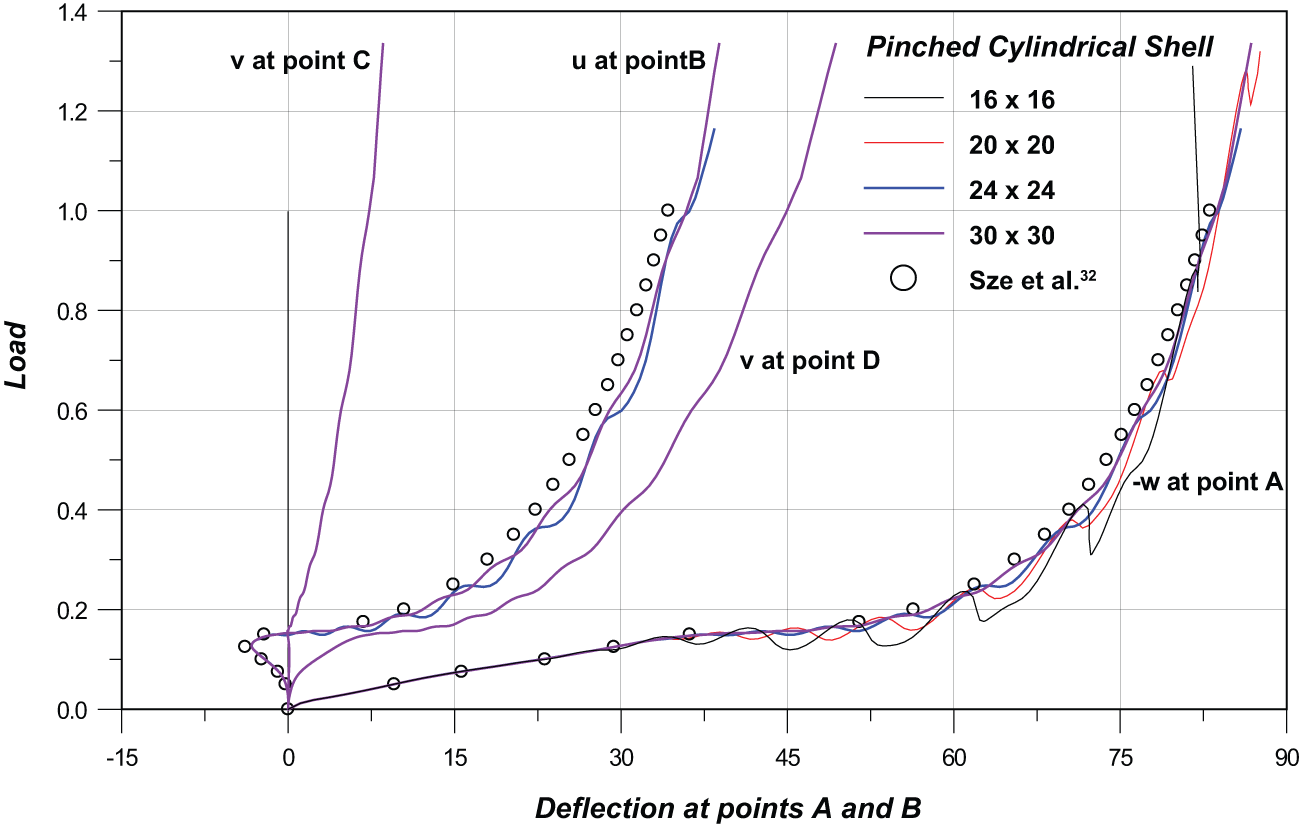
Load–deflection curves for the pinched cylindrical shell.
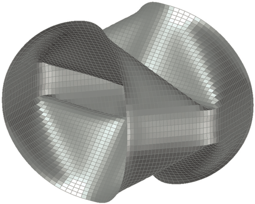
Deformed configuration of the pinched cylindrical shell (24 × 24 mesh) for
Conclusion
The finite element formulation of an improved nine-node shell element is presented for the solution of geometrically nonlinear problems of annular plates, cylindrical, and spherical shells. Geometrically nonlinear analysis of shells using an ELF is proposed. To overcome the limit in the very thin plates and shells, shear and membrane locking is avoided using assumed natural strains. The stress values are required in the formation of the internal force vector and the element tangent stiffness matrix. To avoid the adverse effect of inaccurate stresses on the finite element solution, better stress evaluation method should be adopted. To achieve this goal, strain interpolation scheme similar to the one used in the computation of linear stiffness matrix is first employed for the strain evaluation. Then, based on the interpolated strain field, stresses at integration points are calculated. The numerical results available show that due to such a treatment, the element performance in solving nonlinear problems with distorted mesh can be greatly improved. The present shell element formulation is based on refined first-order transverse shear deformation theory, which results in parabolic through-thickness distribution of the transverse shear strains and stresses. It eliminates the need for shear correction factors in the first-order theory. The scheme for finite rotation of shell normal is used to remove the limitation on magnitude of the rotational increment in each load step in geometrically nonlinear analysis. A full Gauss integration scheme is applied for the evaluation of the membrane, bending, shear, and torsional stiffness. The present solutions show very good agreement with the other numerical solutions. Especially, the annular plate and cylindrical shells may provide the benchmark to test the results of geometrically nonlinear analysis for shell structures.
It should be pointed out that the development of an “absolutely” good element is impossible and one has to be satisfied with those possessing certain desirable properties. It can be expected that the study reported will contribute to further investigation of different approaches for finite element improvement, and thereby to the development of more effective finite elements for engineering applications.
Footnotes
Acknowledgements
The authors would like to express profound gratitude to Prof. W. Kanok-Nukulchai in AIT for his encouragement while preparing this article.
Academic Editor: Stephane PA Bordas
Declaration of conflicting interests
The authors declare that there is no conflict of interests regarding the publication of this article.
Funding
This work was supported by the National Research Foundation of Korea (NRF) grant funded by the Korea Government (MEST) (No. 2011-0028531).