Research on robot manipulator uncalibrated visual serving under two-camera bi-axial parallel vision configuration

Abstract

This article presents a two-camera bi-axial parallel vision configuration to realize robot manipulator uncalibrated visual serving. The intrinsic and extrinsic parameters of the camera and the model of robot manipulator are not known, as well as without real-time computes the inverse of image Jacobian when image-based dynamic control of a robot manipulator in this article. First, the proposed vision configuration is applied to transform the Cartesian posture information into the point and angle parameters in the two image planes. After that, a qualitative mathematical model was established which analyzes the relationship between the feature point and line of the robot manipulator in the Cartesian space and the corresponding specific point and angle in the image plane. In addition, the monotonic property of the point and line features in the mathematic model has been proved. Then, the controller was designed based on image and realized the five-degrees of freedom of the robot manipulator uncalibrated visual serving control in the simulation platform. Moreover, the Lyapunov theory was used to prove the global asymptotic stability of proposed method in the image plane. Finally, the proposed method was compared with the method of image Jacobian matrix in the actual platform experiment, and the comparative experiment results show the effectiveness of the robot manipulator uncalibrated visual serving under the proposed vision configuration.

Introduction

Robot manipulator uncalibrated visual serving is the method that drives the robot manipulator move to the desired posture through real-time accessing and updating image feature changes in the image plane of camera, as well as it has no explicit to calculate the internal and external parameters of the camera. ¹ According to the posture relations between the camera and the robot manipulator in the Cartesian space, the visual serving relationship has been divided into eye-in-hand and eye-to-hand. The eye-in-hand is a camera mounted on the end of the robot manipulator and the eye-to-hand is the camera fixed in the Cartesian space. Moreover, the visual serving system can be divided into monocular vision system, binocular vision system, and multi-purpose vision system on the basis of the number of cameras.^2,3 The vision configuration can directly affect the point and line feature projecting on the image plane in binocular vision system. In our experience, a suitable two-camera configuration can transform the Cartesian posture information into the image feature information in the two image planes, and then it can reduce the difficulty of robot manipulator uncalibrated visual serving control in the Cartesian space.

The two-camera orthogonal vision configuration can obtain the posture information of robot manipulator in the Cartesian space. Meanwhile, the orthogonal vision configuration has many successful application cases. For instance, Wang et al. ⁴ decomposed robot manipulator movement into the position parameter in two-camera planes and the robot manipulator succeeded in tracking the circular path. In the article by Chen et al., ⁵ the automatic marking control system with the orthogonal vision configuration is successfully applied for the automatic marking of gas bottles. In the article by Xu et al., ⁶ Harbin Institute of Technology used the orthogonal vision configuration to develop the microscopic visual micro-manipulator control system, and it has been successfully used in optical fiber butt. Although the orthogonal vision configuration can avoid estimating depth information from the image feature of the camera image plane, but it need to be strictly orthogonal in order to guide the robot manipulator to complete the task. Qian et al. ⁷ achieved robot manipulator precisely tracking the moving object under the eye-in-hand and eye-to-hand vision configurations. Pan et al. ⁸ established the nonlinear visual mapping model between the Cartesian space and the image plane, and they designed a controller based on artificial neural network to eliminate the tracking error. Recently, Liu et al. ⁹ used Kalman filter algorithm to estimate image Jacobian matrix and realized the five-degrees of freedom of robot manipulator uncalibrated visual serving control in MATLAB simulation. Assa et al. ¹⁰ employed the weighted average data fusion method and the extended Kalman filter algorithm to estimate the posture of robot manipulator in the Cartesian space in order to improve the robustness of the controller. Obviously, previous works^7–10 can achieve robot manipulator uncalibrated visual serving control, but it requires a lot of math or complex nonlinear mapping model. Chang et al. ¹¹ calibrated the relationship between the camera and robot manipulator in advance, and robot manipulator realized automated assembly cell phone’s cover with eye-in-hand vision configuration. Wang et al. ¹² used stereo vision to obtain the target depth information and to grab any object in the Cartesian space. However, the articles by Chang et al. ¹¹ and Wang et al. ¹² calibrated the relationship between camera and robot manipulator, and the relationship is related to the controller whether it is able to stabilize convergence or not.

This article proposed a two-camera bi-axis parallel vision configuration, which neither needs two cameras strictly orthogonal nor calculates the image Jacobian or estimates nonlinear mapping model. Moreover, the simulation and experiment realized the five-degrees of freedom of robot manipulator uncalibrated visual serving control.

Vision configuration

Two-camera bi-axial parallel vision configuration

Ideally, two cameras use orthogonal vision configuration, as shown in Figure 1, in which camera 1 and camera 2 are mutually orthogonal in the xy plane of the Cartesian space. But in Figure 1, vision configuration has certain limitations in some engineering applications, for instance, two cameras cannot be completely orthogonal in the same plane. Therefore, this article proposed a two-camera bi-axial parallel vision configuration, as shown in Figure 2, which is based on the orthogonal vision configuration. In the proposed vision configuration, the x axis of camera 1 is parallel to the x axis of the Cartesian space and the x axis of camera 2 is parallel to the y axis of the Cartesian space. besides, camera 1 rotating around x axis is ψ₁ and camera 2 rotating around y axis is ψ₂. It should be pointed out that the proposed vision configuration is not to reconstruct the posture of robot manipulator in the Cartesian space, but to compensate the depth information of the target feature and decompose robot manipulator movement in the Cartesian space into the image feature information in the two image planes. Compared with the orthogonal vision configuration, the proposed vision configuration is still able to realize robot manipulator uncalibrated visual serving control task and achieve an excellent control effect.

Figure 1.

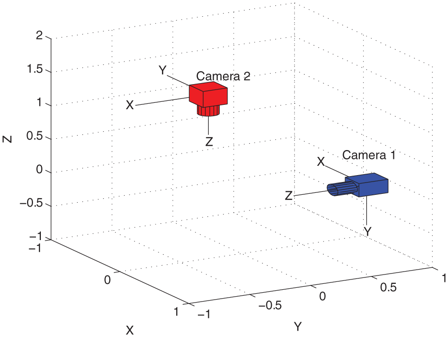
The orthogonal vision configuration.

Figure 2.

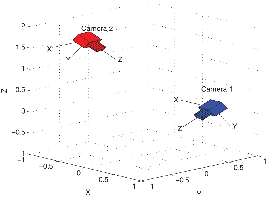
The bi-axial parallel vision configuration.

Camera model

The pinhole image model is commonly used to represent the camera model in machine vision, as shown in Figure 3, which is referred to the central perspective projection model.^6,13 Denote point P coordinates in the Cartesian space as (X_w, Y_w, Z_w) and the coordinates in the camera coordinate as (X_c, Y_c, Z_c).

Figure 3.

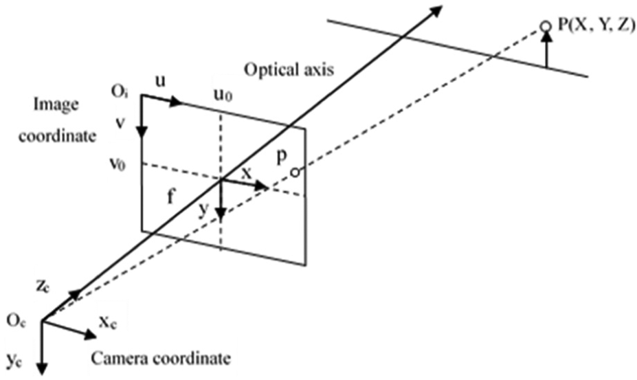
The central perspective model.

Denote the coordinates of point in the imaging plane as (x, y) and f as the focal length of the camera. Represent the pixel coordinates of the image plane by (u, v), and (u₀, v₀) indicates the main center point of the pixel coordinates. According to the central perspective projection model, equation (1) stands for the point P (X_c, Y_c, Z_c) projected onto the imaging plane

$$x=f\frac{X_c}{Z_c},y=f\frac{Y_c}{Z_c}$$

(1)

Note that each pixel’s physical size in the u axis and v axis of the image plane is d_x and d_y, respectively. Then, the imaging plane’s coordinates (x, y) change into the pixel coordinates of image plane (u, v)

$$u=\frac{x}{\mathrm{dx}}+u_0,v=\frac{y}{\mathrm{dy}}+v_0$$

(2)

By equations (1) and (2), the transformation from the imaging plane’s coordinates to the pixel coordinates in the image plane can be represented by equation (3)

$$u={\alpha }_x\frac{X_c}{Z_c}+u_0,v={\alpha }_y\frac{Y_c}{Z_c}+v_0$$

(3)

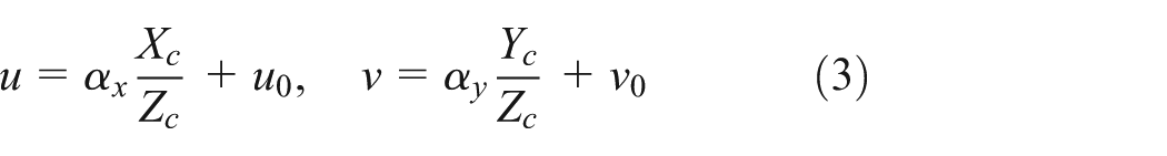
where a_x = f/d_x and a_y = f/d_y are the amplification factors in the x axis and y axis from the imaging plane to the image plane, respectively. The parameters (a_x, a_y, u₀, v₀) are the structural parameters only related to the camera itself.

In this article, the xyz order’s rotation matrix of Euler angle was selected to stand for rigid body’s posture in the Cartesian space. ¹⁴ The parameters (ψ, θ, φ) are defined to represent the angle of rigid body rotating around the x, y, and z axes, respectively. ¹⁴ Therefore, the rotation matrixes R_x , R_y , and R_z in OpenCv are shown in equation (4)

$$\begin{array}{c}{R}_x=\left[\begin{array}{ccc}1\hfill & 0\hfill & 0\hfill \\ \multicolumn{1}{c}{0}& \cos \psi \hfill & \sin \psi \hfill \\ \multicolumn{1}{c}{0}& -\sin \psi \hfill & \cos \psi \hfill \end{array}\right],\hfill \\ R_y=\left[\begin{array}{ccc}\cos \theta \hfill & 0\hfill & -\sin \theta \hfill \\ \multicolumn{1}{c}{0}& 1\hfill & 0\hfill \\ \multicolumn{1}{c}{\sin \theta }& 0\hfill & \cos \theta \hfill \end{array}\right],\hfill \\ R_z=\left[\begin{array}{ccc}\cos \varphi \hfill & \sin \varphi \hfill & 0\hfill \\ \multicolumn{1}{c}{-\sin \varphi }& \cos \varphi \hfill & 0\hfill \\ \multicolumn{1}{c}{0}& 0\hfill & 1\hfill \end{array}\right]\hfill \end{array}$$

(4)

According to equation (4) and the vision configuration in Figure 2, the rotation matrix and translation vector of camera 1 are R_cam1 and T_cam1 , respectively, which were expressed as equation (5)

$$\begin{array}{c}\multicolumn{1}{c}{R_{\mathrm{cam}1}=R_x(-90\circ -{\psi }_1)R_z(-180\circ )}\\ =\left[\begin{array}{ccc}-1\hfill & 0\hfill & 0\hfill \\ \multicolumn{1}{c}{0}& \sin {\psi }_1\hfill & -\cos {\psi }_1\hfill \\ \multicolumn{1}{c}{0}& -\cos {\psi }_1\hfill & -\sin {\psi }_1\hfill \end{array}\right],\hfill \\ \multicolumn{1}{c}{T_{\mathrm{cam}1}=[x_1,y_1,z_1]}\end{array}$$

(5)

where ψ₁ is the tilt angle of camera 1 and the parameters (x₁, y₁, z₁) are the position of camera 1 in the Cartesian space. Similarly, the rotation matrix and translation vector of camera 2 are referred to as R_cam2 and T_cam2 , which were expressed by equation (6)

$$\begin{array}{c}{R}_{\mathrm{cam}2}=R_x(-180\circ +{\psi }_2)R_z(-90\circ )\hfill \\ =\left[\begin{array}{ccc}0\hfill & -1\hfill & 0\hfill \\ \multicolumn{1}{c}{-\cos {\psi }_2}& 0\hfill & -\sin {\psi }_2\hfill \\ \multicolumn{1}{c}{\sin {\psi }_2}& 0\hfill & -\cos {\psi }_2\hfill \end{array}\right],T_{\mathrm{cam}2}=[x_2,y_2,z_2]\hfill \end{array}$$

(6)

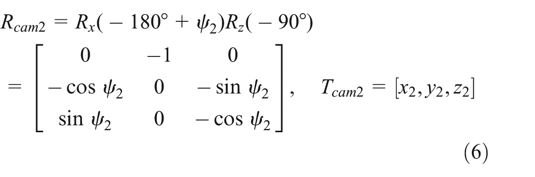
where ψ₂ is the angle that camera 2 rotates around the y axis and the variables (x₂, y₂, z₂) are the position of camera 2 in the Cartesian space.

Therefore, the homogeneous coordinate transformation from the Cartesian coordinates (X_w, Y_w, Z_w) to the camera coordinates (X_c, Y_c, Z_c) can be represented by equation (7)

$$\left[\begin{array}{c}{X}_c\hfill \\ \multicolumn{1}{c}{Y_c}\\ \multicolumn{1}{c}{Z_c}\\ \multicolumn{1}{c}{1}\end{array}\right]=\left[\begin{array}{cc}{R}_{\mathrm{cam}}\hfill & T_{\mathrm{cam}}\hfill \\ \multicolumn{1}{c}{0}& 1\hfill \end{array}\right]\left[\begin{array}{c}{X}_w\hfill \\ \multicolumn{1}{c}{Y_w}\\ \multicolumn{1}{c}{Z_w}\\ \multicolumn{1}{c}{1}\end{array}\right]$$

(7)

where R_cam is a 3 × 3 matrix determined by the intrinsic parameters of the camera and T_cam is a 1 × 3 vector composed by the external parameters of the camera.

Image feature selection

Image feature’s selection and extraction directly determine the controller design and the robustness of the closed-loop control system. Image feature frequently used is point, line, angle, area, optical flow field, or Fourier descriptor. Local image feature, for instance, point or angle, is relatively easy to extract and adapt to changing environment. Hence, this article selects a point and an angle as the image feature to indicate that robot manipulator moves in the Cartesian space. However, the number of image features in this article must be greater than or equal to the degrees of freedom controlled by the robot manipulator in order to achieve robot manipulator uncalibrated visual serving control task. Therefore, this article needs to select five image features at least for the purpose of realizing the five-degrees of freedom of robot manipulator uncalibrated visual serving control. According to the above discussion, the image feature set of this article is (u1_p1, v1_p1, u2_p1, v2_p1, θ₁, θ₂). The parameters (u1_p1, v1_p1) are the pixel coordinates of point P in camera 1 and θ₁ is the angle θ between line p₁p₂ and u axis in camera 1. In addition, the parameters (u2_p1, v2_p1) are the pixel coordinates of point P in camera 2 and θ₂ is the angle θ between line p₁p₂ and u axis in camera 2. The abstract projection model of image feature set is shown in Figure 4. Moreover, we selected the magenta and orange color block on the robot manipulator end in order to represent the image feature of a point and an angle in the actual platform experiment, and the actual projection model of image feature set is shown in Figure 5.

Figure 4.

The abstract projection model of image feature set.

Figure 5.

The actual projection model of image feature set.

Vision model analysis and controller design

Vision model analysis

Robot manipulator movement is synthesized by the translational component of the x or y or z axis in the Cartesian space. Thus, it is of great significance to analyze the changing trend of the specific feature in the image plane when robot manipulator translates along the x or y or z axis of the Cartesian space. Denote the robot manipulator end’s point by P and its coordinates as P_w = (X_w, Y_w, Z_w) in the Cartesian space. The parameters P_c1 =  (X_c1, Y_c1, Z_c1) and P_c2 =  (X_c2, Y_c2, Z_c2) are the coordinates of point P in camera 1 and camera 2 coordinates, respectively, as well as P_img1 =  (u₁,v₁) and P_img2 =  (u₂,v₂) are the projection coordinates of point P in the image plane of camera 1 and camera 2. Note that the parameters (P′_w, P′_c1, P′_c2, P′_img1, P′_img2) represent the feature point coordinates of robot manipulator end in the previous time and the parameters (P_w, P_c1, P_c2, P_img1, P_img2) are the feature point’s coordinates of the current time. To guarantee the image feature always within the visual area of camera 1 and camera 2, the parameters Z_c and Z′_c must satisfy Z_c >  0 and Z′_c >  0. With reference to the camera model, a_x and ay are the physical parameters of the camera, and they meet the condition a_x and a_y. According to the two-camera bi-axis parallel vision configuration, a qualitative mathematical model has been established in this article and it has the following properties.

Property 1

The pixel coordinate function u₁ = f (X_w) of camera 1 image plane has a monotonically increasing or decreasing nature when the robot manipulator end’s feature point translates ΔX_w along the X_w axis of the Cartesian space.

Proof

The current coordinates of feature point are P_w = (X′_w+ΔX_w, Y′_w, Z′_w) after the robot manipulator translates ΔX_w along the X_w axis of the Cartesian space. Then, equation (2), equation (3), and point coordinates P_w are substituted into equation (7). After that, the feature point’s coordinates P_c1 and P_c2 in camera 1 and camera 2 coordinate can result in formula (8)

$$\begin{array}{c}{P}_{c1}=({X\prime }_{c1}-\mathrm{\Delta }{X}_w,{Y\prime }_{c1},{Z\prime }_{c1})\hfill \\ \multicolumn{1}{c}{P_{c2}=({X\prime }_{c2},{Y\prime }_{c2}-\mathrm{\Delta }{X}_w\cos {\psi }_2,{Z\prime }_{c2}+\mathrm{\Delta }{X}_w\sin {\psi }_2)}\end{array}$$

(8)

By combining equations (5) and (8), the difference between the previous and the current pixel coordinates in the image plane of camera 1 is formula (9)

$$\{\begin{array}{c}\mathrm{\Delta }{u}_1=u_1-{u\prime }_1={\alpha }_{x1}(\frac{X_{c1}}{Z_{c1}}-\frac{{X\prime }_{c1}}{{Z\prime }_{c1}})={\alpha }_{x1}\frac{-\mathrm{\Delta }{X}_w}{{Z\prime }_{c1}}\hfill \\ \multicolumn{1}{c}{\mathrm{\Delta }{v}_1=v_1-{v\prime }_1={\alpha }_{y1}(\frac{Y_{c1}}{Z_{c1}}-\frac{{Y\prime }_{c1}}{{Z\prime }_{c1}})=0}\\ \multicolumn{1}{c}{\mathrm{\Delta }{u}_2=u_2-{u\prime }_2={\alpha }_{x2}(\frac{X_{c2}}{Z_{c2}}-\frac{{X\prime }_{c2}}{{Z\prime }_{c2}})={\alpha }_{x2}\frac{-{X\prime }_{c2}\mathrm{\Delta }{X}_w\sin {\psi }_2}{{Z\prime }_{c2}({Z\prime }_{c2}+\mathrm{\Delta }{X}_w\sin {\psi }_2)}}\\ \multicolumn{1}{c}{\mathrm{\Delta }{v}_2=v_2-{v\prime }_2={\alpha }_{y2}(\frac{Y_{c2}}{Z_{c2}}-\frac{{Y\prime }_{c2}}{{Z\prime }_{c2}})={\alpha }_{y2}\frac{(-{Z\prime }_{c2}\cos {\psi }_2-{Y\prime }_{c2}\sin {\psi }_2)\mathrm{\Delta }{X}_w}{{Z\prime }_{c2}({Z\prime }_{c2}+\mathrm{\Delta }{X}_w\sin {\psi }_2)}}\end{array}$$

(9)

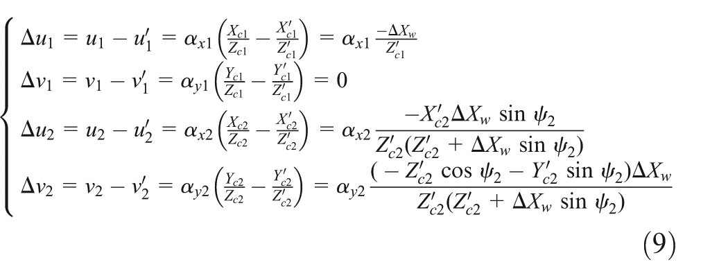
For a_x1> 0 and Z′_c1> 0, there is

$$\begin{array}{cc}\forall X_w,\hfill & \mathrm{\Delta }{X}_w>0\Rightarrow \mathrm{\Delta }{u}_1<0\hfill \\ \mathrm{\Delta }{X}_w<0\Rightarrow \mathrm{\Delta }{u}_1>0\hfill \end{array}$$

(10)

Therefore, the function u₁ = f (X_w) has a monotonically increasing or decreasing nature which is analyzed by formula (10).

Property 2

The pixel coordinates function u₂ = f (Y_w) of camera 2 image plane has a monotonically increasing or decreasing nature when robot manipulator end’s feature point translates ΔY_w along the Y_w axis of the Cartesian space.

Proof

Similarly, the current coordinates of feature point are P_w = (X′_w, Y′_w+ΔY_w, Z′_w) after the robot manipulator translates ΔY_w along the Y_w axis of the Cartesian space. Afterward, equation (2), equation (3), and point coordinates P_w are substituted into equation (7). Then, the feature point’s coordinates P_c1 and P_c2 in camera 1 and camera 2 can be expressed by formula (11)

$$\begin{array}{c}{P}_{c1}=({X\prime }_{c1},{Y\prime }_{c1}+\mathrm{\Delta }{Y}_w\sin {\psi }_1,{Z\prime }_{c1}-\mathrm{\Delta }{Y}_w\cos {\psi }_1)\hfill \\ \multicolumn{1}{c}{P_{c2}=({X\prime }_{c2}-\mathrm{\Delta }{Y}_w,{Y\prime }_{c2},{Z\prime }_{c2})}\end{array}$$

(11)

From equations (5) and (11), the difference pixel coordinates of camera 2 between the previous position and the current position can be related as formula (12)

$$\{\begin{array}{c}\mathrm{\Delta }{u}_1=u_1-{u\prime }_1={\alpha }_{x1}(\frac{X_{c1}}{Z_{c1}}-\frac{{X\prime }_{c1}}{{Z\prime }_{c1}})={\alpha }_{x1}\frac{{X\prime }_{c1}\mathrm{\Delta }{Y}_w\cos {\psi }_1}{{Z\prime }_{c1}({Z\prime }_{c1}-\mathrm{\Delta }{Y}_w\cos {\psi }_1)}\hfill \\ \multicolumn{1}{c}{\mathrm{\Delta }{v}_1=v_1-{v\prime }_1={\alpha }_{y1}(\frac{Y_{c1}}{Z_{c1}}-\frac{{Y\prime }_{c1}}{{Z\prime }_{c1}})={\alpha }_{y1}\frac{({Z\prime }_{c1}\sin {\psi }_1+{Y\prime }_c\cos {\psi }_1)\mathrm{\Delta }{Y}_w}{{Z\prime }_{c1}({Z\prime }_{c1}-\mathrm{\Delta }{Y}_w\cos {\psi }_1)}}\\ \multicolumn{1}{c}{\mathrm{\Delta }{u}_2=u_2-{u\prime }_2={\alpha }_{x2}(\frac{X_{c2}}{Z_{c2}}-\frac{{X\prime }_{c2}}{{Z\prime }_{c2}})={\alpha }_{x2}\frac{-\mathrm{\Delta }{Y}_w}{{Z\prime }_{c2}}}\\ \multicolumn{1}{c}{\mathrm{\Delta }{v}_2=v_2-{v\prime }_2={\alpha }_{y2}(\frac{Y_{c2}}{Z_{c2}}-\frac{{Y\prime }_{c2}}{{Z\prime }_{c2}})=0}\end{array}$$

(12)

For a_x2> 0 and Z′_c2> 0, there is

$$\begin{array}{cc}\forall Y_w,\hfill & \mathrm{\Delta }{Y}_w>0\Rightarrow \mathrm{\Delta }{u}_2<0\hfill \\ \mathrm{\Delta }{Y}_w<0\Rightarrow \mathrm{\Delta }{u}_2>0\hfill \end{array}$$

(13)

Thus, the function u₂ = f (Y_w) has a monotonically increasing or decreasing nature according to formula (12).

Property 3

The pixel coordinates function v₁ = f (Z_w) of camera 1 image plane has a monotonically increasing or decreasing nature when robot manipulator end’s feature point translates ΔZ_w along the Z_w axis of the Cartesian space.

Proof

The proof process is similar to property 1 and property 2. First, the current coordinates of feature point are P_w = (X′_w, Y′_w, Z′_w+ΔZ_w) after robot manipulator translates ΔZ_w along the Z_w axis of the Cartesian space. After that, there is formula (14) to indicate the feature point’s coordinates P_c1 and P_c2 in camera 1 and camera 2 coordinates by substituting equation (2), equation (3), and point coordinates P_w into equation (7)

$$\begin{array}{c}\multicolumn{1}{c}{P_{c1}=({X\prime }_{c1},{Y\prime }_{c1}-\mathrm{\Delta }{Z}_w\cos {\psi }_1,{Z\prime }_{c1}-\mathrm{\Delta }{Z}_w\sin {\psi }_1)}\\ \multicolumn{1}{c}{P_{c2}=({X\prime }_{c2},{Y\prime }_{c2}-\mathrm{\Delta }{Z}_w\sin {\psi }_2,{Z\prime }_{c2}-\mathrm{\Delta }{Z}_w\cos {\psi }_2)}\end{array}$$

(14)

By combining equations (5) and (14), the difference pixel coordinates of camera 1 between the previous position and the current position can be given by formula (15)

$$\{\begin{array}{c}\mathrm{\Delta }{u}_1=u_1-{u\prime }_1={\alpha }_{x1}(\frac{X_{c1}}{Z_{c1}}-\frac{{X\prime }_{c1}}{{Z\prime }_{c1}})={\alpha }_{x1}\frac{{X\prime }_{c1}\mathrm{\Delta }{Z}_w\sin {\psi }_1}{{Z\prime }_{c1}({Z\prime }_{c1}-\mathrm{\Delta }{Z}_w\sin {\psi }_1)}\hfill \\ \multicolumn{1}{c}{\mathrm{\Delta }{v}_1=v_1-{v\prime }_1={\alpha }_{y1}(\frac{Y_{c1}}{Z_{c1}}-\frac{{Y\prime }_{c1}}{{Z\prime }_{c1}})={\alpha }_{y1}\frac{({Y\prime }_{c1}\sin {\psi }_1-{Z\prime }_{c1}\cos {\psi }_1)\mathrm{\Delta }{Z}_w}{{Z\prime }_{c1}({Z\prime }_{c1}-\mathrm{\Delta }{Z}_w\sin {\psi }_1)}}\\ \multicolumn{1}{c}{\mathrm{\Delta }{u}_2=u_2-{u\prime }_2={\alpha }_{x2}(\frac{X_{c2}}{Z_{c2}}-\frac{{X\prime }_{c2}}{{Z\prime }_{c2}})={\alpha }_{x2}\frac{{X\prime }_{c2}\mathrm{\Delta }{Z}_w\cos {\psi }_2}{{Z\prime }_{c2}({Z\prime }_{c2}-\mathrm{\Delta }{Z}_w\cos {\psi }_2)}}\\ \multicolumn{1}{c}{\mathrm{\Delta }{v}_2=v_2-{v\prime }_2={\alpha }_{y2}(\frac{Y_{c2}}{Z_{c2}}-\frac{{Y\prime }_{c2}}{{Z\prime }_{c2}})={\alpha }_{y2}\frac{({Y\prime }_{c2}\cos {\psi }_2-{Z\prime }_{c2}\sin {\psi }_2)\mathrm{\Delta }{Z}_w}{{Z\prime }_{c2}({Z\prime }_{c2}-\mathrm{\Delta }{Z}_w\cos {\psi }_2)}}\end{array}$$

(15)

Assuming the camera’s resolution is R₁ × R₂ and the camera sensor size is S₁ × S₂, there is formula (16) according to the pinhole image model

$$\{\begin{array}{c}{v}_0=R_2/2\hfill \\ \mathrm{dy}=S_2/R_2\hfill \\ a_y=f/\mathrm{dy}=f\times R_2/S_2\hfill \end{array}$$

(16)

From formulas (3) and (16), we obtain

$$\frac{Y_c}{Z_c}=\frac{((v-R_2/2)\times S_2)}{(R_2\times f)};v\in [0,R_2]$$

(17)

where (v, v₀) are the pixel coordinates and f is the focal length of the camera. It should be pointed out that the molecular of formula (17) is far greater than the denominator with respect to the parameter of the high-resolution industrial camera. Besides, the tilt angle of camera 1 ψ₁(0 ≤ ψ₁ ≤ 20) is small and ΔZ_w is a very small amount of translation. Therefore, the simplification of formula (18) exists when the tilt angle of camera 1 ψ₁ is small

$$\begin{array}{c}\frac{({Y\prime }_{c1}\sin {\psi }_1-{Z\prime }_{c1}\cos {\psi }_1)}{{Z\prime }_{c1}}\approx -\cos {\psi }_1\hfill \\ {Z\prime }_{c1}-\mathrm{\Delta }{Z}_w\sin {\psi }_1\approx {Z\prime }_{c1}\hfill \end{array}$$

(18)

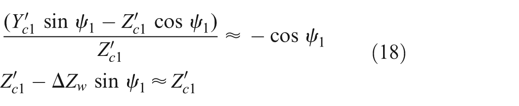
By submitting formula (18) into formula (15), formula (15) can be re-written as follows

$$\{\begin{array}{c}\mathrm{\Delta }{u}_1=u_1-{u\prime }_1={\alpha }_{x1}(\frac{X_{c1}}{Z_{c1}}-\frac{{X\prime }_{c1}}{{Z\prime }_{c1}})={\alpha }_{x1}\frac{{X\prime }_{c1}\mathrm{\Delta }{Z}_w\sin {\psi }_1}{{Z\prime }_{c1}^2}\hfill \\ \multicolumn{1}{c}{\mathrm{\Delta }{v}_1=v_1-{v\prime }_1={\alpha }_{y1}(\frac{Y_{c1}}{Z_{c1}}-\frac{{Y\prime }_{c1}}{{Z\prime }_{c1}})={\alpha }_{y1}\frac{-\mathrm{\Delta }{Z}_w\cos {\psi }_1}{{Z\prime }_{c1}}}\\ \multicolumn{1}{c}{\mathrm{\Delta }{u}_2=u_2-{u\prime }_2={\alpha }_{x2}(\frac{X_{c2}}{Z_{c2}}-\frac{{X\prime }_{c2}}{{Z\prime }_{c2}})={\alpha }_{x2}\frac{{X\prime }_{c2}\mathrm{\Delta }{Z}_w\cos {\psi }_2}{{Z\prime }_{c2}({Z\prime }_{c2}-\mathrm{\Delta }{Z}_w\cos {\psi }_2)}}\\ \multicolumn{1}{c}{\mathrm{\Delta }{v}_2=v_2-{v\prime }_2={\alpha }_{y2}(\frac{Y_{c2}}{Z_{c2}}-\frac{{Y\prime }_{c2}}{{Z\prime }_{c2}})={\alpha }_{y2}\frac{({Y\prime }_{c2}\cos {\psi }_2-{Z\prime }_{c2}\sin {\psi }_2)\mathrm{\Delta }{Z}_w}{{Z\prime }_{c2}({Z\prime }_{c2}-\mathrm{\Delta }{Z}_w\cos {\psi }_2)}}\end{array}$$

(19)

For a_y1> 0 and Z′_c1> 0, there is

$$\begin{array}{cc}\forall Z_w,\hfill & \mathrm{\Delta }{Z}_w>0\Rightarrow \mathrm{\Delta }{v}_1<0\hfill \\ \mathrm{\Delta }{Z}_w<0\Rightarrow \mathrm{\Delta }{v}_1>0\hfill \end{array}$$

(20)

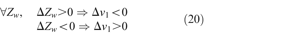
According to formula (19), the function v₁ = f (Z_w) has a monotonically increasing or decreasing nature.

Property 4

The line feature of the robot manipulator end composed by two feature points, and between the line feature and the z axis of the Cartesian space has an angle $\theta$ . The unit vector v is the projection of line feature in the xoy plane of the Cartesian space, and between the unit vector and the i axis of the Cartesian space has an angle $\alpha$ . When the angle $\alpha$ changes monotonously, the angle θ has a piecewise monotonic characteristic.

Proof

The posture of the line can use the spherical coordinates ϕ and θ $(0\le \phi <2\pi ,0\le \theta <\pi )$ to represent in the Cartesian space. ¹⁵ The spherical coordinate is shown in Figure 6.

Figure 6.

The spherical coordinate.

Note that unit vector u represents the posture of the target line in the Cartesian space

$$\mathit{u}=\left[\begin{array}{c}\cos \varphi \sin \theta \hfill \\ \multicolumn{1}{c}{\sin \varphi \sin \theta }\\ \multicolumn{1}{c}{\cos \theta }\end{array}\right]$$

(21)

Denote the projection vector of unit vector u in the yoz plane of the spherical coordinate as $v=(\sin \varphi \sin \theta ,\cos \theta )$ and the angle between vector v and the z axis of the Cartesian space as a. Then, the vector angle formula (22) is as follows

$$\cos \alpha =\frac{1}{\sqrt{(\sin \varphi \tan \theta {)}^2+1}}$$

(22)

Suppose that the angle θis a function of a, formula (22) can be re-written as

$$\theta =f(\alpha )=\mathrm{arctg}\left(\frac{\tan \alpha }{\sin \varphi }\right)$$

(23)

The function y = arctg(x) is a monotonically increasing function, and the monotonic of $x=\tan a/\sin \varphi$ is decided by the quadrant of angle φ. Thus, there is formula (24) according to the defined region of function tan(a) and the monotonicity of the composite function

$$\begin{array}{c}\begin{array}{cc}\forall \varphi \in (0,\pi ),\hfill & \mathrm{\Delta }\alpha >0\Rightarrow \mathrm{\Delta }\theta >0\hfill \\ \mathrm{\Delta }\alpha <0\Rightarrow \mathrm{\Delta }\theta <0\hfill \end{array}\hfill \\ \begin{array}{cc}\forall \varphi \in (\pi ,2\pi ),\hfill & \mathrm{\Delta }\alpha >0\Rightarrow \mathrm{\Delta }\theta <0\hfill \\ \mathrm{\Delta }\alpha <0\Rightarrow \mathrm{\Delta }\theta >0\hfill \end{array}\hfill \end{array}$$

(24)

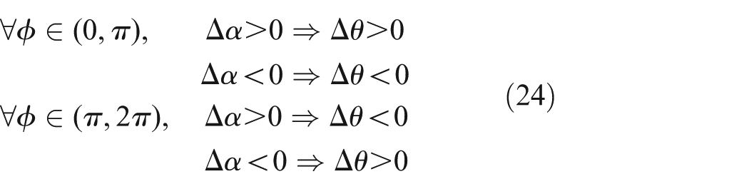
Hence, the monotonicity of function v₁ = f (Z_w) is related to the quadrant of angle φ and it has piecewise monotonic nature.

According to the homogeneity of spherical coordinate notation, between the line feature and the x axis of the Cartesian space has an angle $\theta$ . The unit vector v is the projection of line feature in the xoz plane of the Cartesian space, and between the unit vector and the x axis of the Cartesian space has an angle $\alpha$ . When the angle $\alpha$ changes monotonously, the angle $\theta$ has a piecewise monotonic characteristic. Similarly to be proved, between the line feature and the y axis of the Cartesian space has an angle u. The unit vector v is the projection of line feature in the xoy plane of the Cartesian space, and between the unit vector and the y axis of the Cartesian space has an angle $\alpha$ . When the angle $\alpha$ changes monotonously, the angle $\theta$ has a piecewise monotonic characteristic.

Controller design

Taking the above discussions into account, the robot manipulator translates along the X_w or Y_w or Z_w axis and rotates around the X_w or Z_w in the Cartesian space. After that, the trajectory of feature point in the image plane is shown in Figures 7 and 8. As we have seen in Figure 7, the variables (u₁, u₂, v₁) are the main characteristic variation to reflect robot manipulator translating along the X_w or Y_w or Z_w axis, respectively. Besides, the feature point’s trajectory in the image plane demonstrated the correctness of property 1, property 2, and property 3. Similarly, the angles (θ₁, θ₂) are the main characteristic variation when robot manipulator rotates around the X_w or Z_w axis, respectively, in Figure 8. Moreover, the monotonic of the trajectory in the image plane also proves the validity of property 4.

Figure 7.

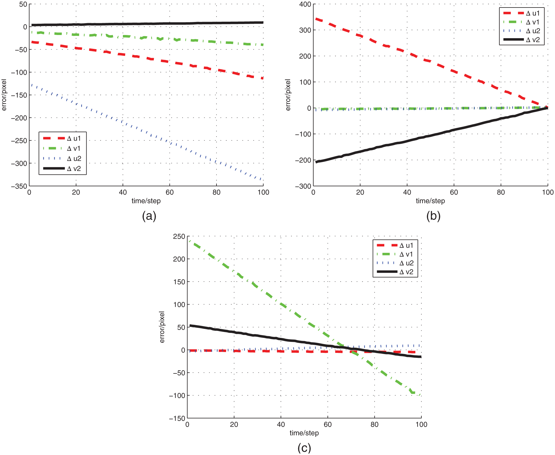
Robot manipulator translates along the (a) x, (b) y, and (c) z axes.

Figure 8.

Robot manipulator rotates around the (a) x and (b) z axes.

According to the experiment trajectory in Figures 7 and 8, the controller selects a main characteristic variation to reflect the robot manipulator translating along or rotating around the X_w or Y_w or Z_w axis in the Cartesian space. Thus, the controller selects the variables (u₁, u₂, v₁) to represent the robot manipulator to translate along the X_w, Y_w, and Z_w axes respectively, and chooses the angles θ₁ and θ₂ to reflect the robot manipulator rotating around the X_w and Z_w axes. For simplicity, the quantitative control model based on the two-camera bi-axial parallel vision configuration can be described by formula (25)

$$\{\begin{array}{c}\mathrm{\Delta }{X}_w=a_1\mathrm{\Delta }{u}_1\hfill \\ \mathrm{\Delta }{Y}_w=a_2\mathrm{\Delta }{u}_2\hfill \\ \mathrm{\Delta }{Z}_w=a_3\mathrm{\Delta }{v}_1\hfill \\ \mathrm{\Delta }{\mathrm{RotX}}_w=a_4\mathrm{\Delta }{\theta }_1\hfill \\ \mathrm{\Delta }{\mathrm{RotZ}}_w=a_5\mathrm{\Delta }{\theta }_2\hfill \end{array}$$

(25)

Based on the quantitative control model above, this article proposed the following controller

$$\tau =K_{p}E+K_i\int {\mathrm{Ed}}_t-K_{d}q\prime (t)+G(q(t))$$

(26)

where E is the 6 × 1 posture error vector in the Cartesian space. The coefficients K_p , K_i , and K_d are the 6 × 6 diagonal matrix. The term q ′(t) is a 6 × 1 vector that represents the joint velocity feedback in the joint space. The last term is to cancel the gravitational force in the robot dynamics.

Stability analysisa

This section analyzes the stability of the robot manipulator under the control of the proposed vision configuration and the controller. According to the analysis and proof in section “Vision model analysis,” we can conclude that the image error asymptotic converge to 0 meaning that the robot manipulator can stably converge to the desired posture in the Cartesian space. Thus, the stability in the image plane is equivalent to the stability of the robot manipulator in the Cartesian space. For simplicity, we assume that the feature point is visible during the motion. Following is the process of stability proof in the Cartesian space.

Proof

It is well-known that the dynamic equation of robot manipulator is equation (27).^16–18

$$H(q(t))q″(t)+V(q(t),q\prime (t))+G(q(t))=\tau$$

(27)

where q(t) is the joint angle of robot manipulator and q ′(t) is a joint velocity vector. H(q(t)) is the mass matrix of the robot manipulator and V(q(t), and q ′(t)) is a centrifugal and coriolis force matrix.

The proposed controller in this article is

$$K_{p}E+K_i\int {\mathrm{Ed}}_t-K_{d}q\prime (t)+G(q(t))=\tau$$

(28)

Introduce the following non-negative energy function V(t)

$$V(t)=\frac{1}{2}q\prime (t{)}^{T}H(q(t))q\prime (t)+\frac{1}{2}(E^T{K}_{p}E+\int E^T{K}_i{\mathrm{Ed}}_t)$$

(29)

From formula (29), the value of V(t) is always positive or 0 when the value of t satisfies t ≥ 0.

By combining formulas (27) and (28), the closed-loop dynamics equation is obtained

$$H(q(t))q″(\mathrm{t})+V(q(t),q\prime (t))=K_{p}E+K_i\int {\mathrm{Ed}}_t-K_{d}q\prime (t)$$

(30)

Multiplying the q ′(t) ^T from the left to formula (27) results in

$$\begin{array}{c}q\prime (t{)}^{T}H(q(t))q″(t)+q\prime (t{)}^{T}V(q(t),q\prime (t))\hfill \\ =q\prime (t{)}^T{K}_{p}E+q\prime (t{)}^T{K}_i\int {\mathrm{Ed}}_t-q\prime (t{)}^T{K}_{d}q\prime (t)\hfill \end{array}$$

(31)

Differentiating the function V(t) in formula (29) results in

$$\begin{array}{c}\multicolumn{1}{c}{V(t)\prime =q\prime (t{)}^{T}H(q(t))q″(t)+\frac{1}{2}q\prime (t{)}^{T}H\prime (q(t))q\prime (t)}\\ -E^T{K}_{p}q\prime (t)-q\prime (t{)}^T{K}_i\int {\mathrm{Ed}}_t\hfill \end{array}$$

(32)

The following equation was established through the structural analysis of Lagrange motion equation^19–21

$$\frac{1}{2}q\prime (t{)}^{T}H\prime (q(t))q\prime (t)=q\prime (t{)}^{T}V(q(t),q\prime (t))$$

(33)

By combining formulas (31)–(33), the derivation of Lyapunov function can be simplified

$$V(t)\prime =-q\prime (t{)}^T{K}_{d}q\prime (t)$$

(34)

Because the parameter of K_d matrix is always positive, the function V’(t) will be always negative. Thus, V(t) meets asymptotically stable in the Cartesian space. In addition, the vectors q ″(t) and q ′(t) should meet with q ″(t) = 0 and q ′(t) = 0 so that V(t) is constant and equal to 0. Then, formula (30) can be re-written as

$$K_{p}E+K_i\int {\mathrm{Ed}}_t=0$$

(35)

Because the matrix K_p and K_i are have non-singularity, there is

$$E=0$$

(36)

Therefore, this article can achieve the global asymptotic stability of robot manipulator in the Cartesian space under the proposed vision configuration and the controller.

Simulation and experiment

Simulation

This article developed the simulation platform in order to verify the validity of the proposed controller under the two-camera bi-axis parallel vision configuration. The simulation platform is shown in Figure 9, which is composed of the three-dimensional (3D) scene platform model in the Open Inventor, the vision module in the OpenCv, and the robot control module in the Orocos. All its modules are open software source that are widely used by scholars. Moreover, the graphical user interface module and the human–machine interaction module are developed by the MFC and DirectInput development kit.

Figure 9.

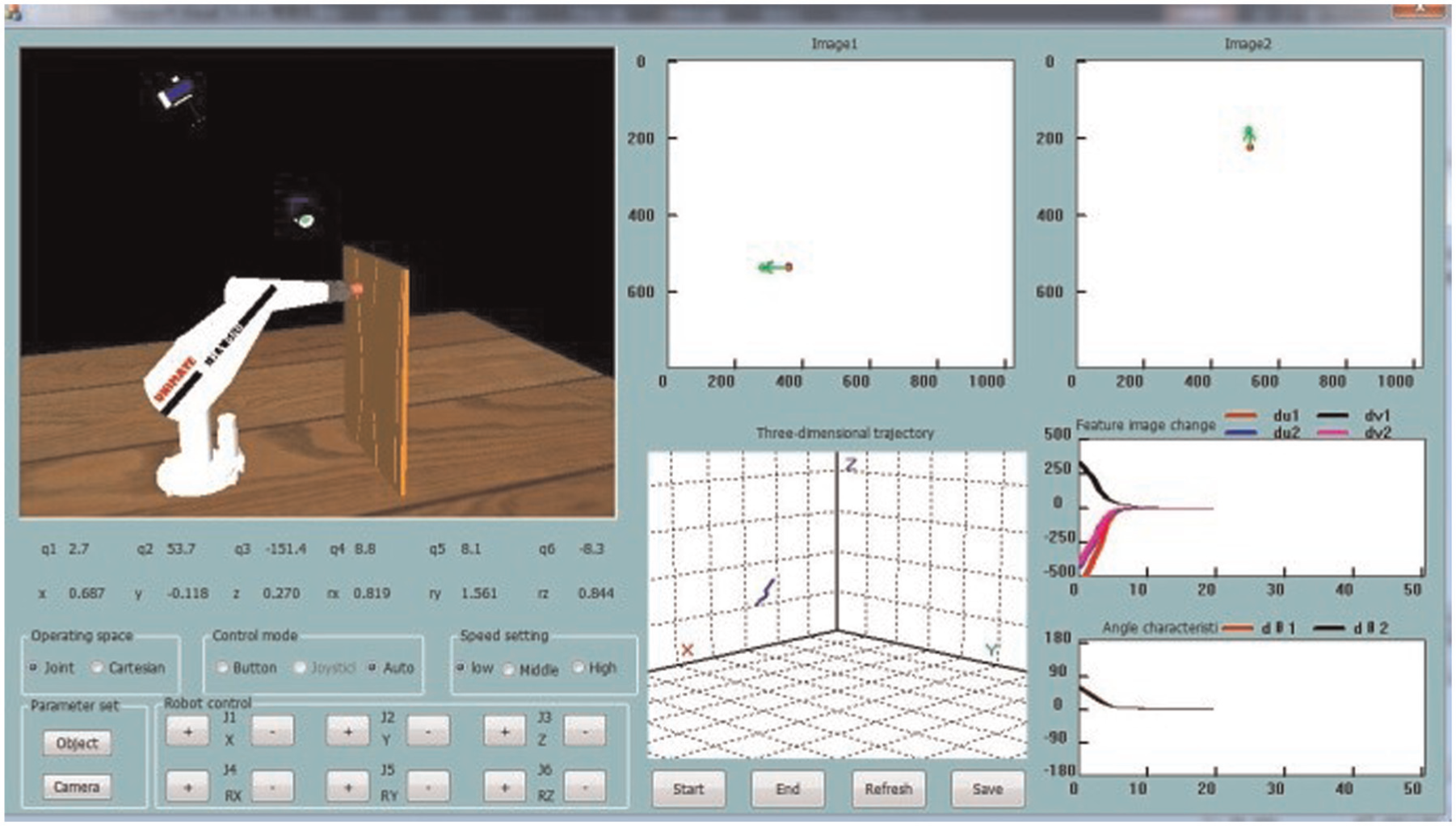
The simulation platform.

The robot manipulator model used in the simulation platform is Puma560. The intrinsic parameters of two cameras are reference to the actual industrial camera that the image resolution is 1024 × 768, the camera sensor size is 4.8 × 3.6, and the focal length is 12 mm. The camera 1 counter-rotates around the x axis of the Cartesian spaceŁ20 degrees and the camera 2 rotates around the y axis of the Cartesian space Ł60 degrees. The extrinsic parameters of two cameras are T_cam1  = (0.4, 0.38, 1.14) and T_cam2  = (0.0, 0.58, 1.40), respectively. In addition, the flow chart of the simulation program is shown in Figure 10, and the actual platform experiment also uses the same flow chart like this.

Figure 10.

The flow chart of the simulation program.

Denote the initial image feature vector in the image plane as (970.9, 178.9, −121.8, 961.0, 624.9, −36.1) and the initial posture of the robot manipulator in the Cartesian space as (242.8, −439.6, 368.7, 46.9, 36.0, 0.0) in the simulation experiment. The desired image feature vector is (387.2, 522.3, 177.4, 527.1 226.4, −96.6) and the expectation posture of robot manipulator is (680.3, −114.1, 269.5, 46.9, 89.2, 52.2). After the simulation, the error curves of image feature and robot manipulator’s posture are as shown in Figures 11 and 12, respectively.

Figure 11.

Image feature error’s curve.

Figure 12.

Robot manipulator pose error’s curve.

After the simulation, the final image feature vector is (386.9, 522.2, 177.4, 527.8, 226.4, −96.7) and the final posture of the robot manipulator in the Cartesian space is (680.6, −114.8, 269.0, 46.9, 89.5, 52.1). As a result, the error vector with respect to the desired image feature is (−0.3, −0.1, 0.0, 0.7, 0.0, −0.1) and the error vector compared with the expectation posture of robot manipulator is (0.3, −0.7, −0.5, 0.0, 0.3, −0.1). According to the error vector, the image feature’s error in the image plane is within 1 pixel or degree and the posture error in the Cartesian space is less than 1 mm or 1°. Besides, the point trajectory in the Cartesian space is shown in Figure 13. In conclusion, the simulation result shows that robot manipulator realized the five-degrees of freedom of robot manipulator uncalibrated visual serving control with minimal error both in the image plane and in the Cartesian space.

Figure 13.

Point trajectory in Cartesian space.

Experiment

This article conducts a comparison experiment in the actual platform in order to verify the effectiveness of the proposed vision configuration. The actual physical platform is shown in Figure 12, which composed by the Denso robot VS-6556, the MV-VS078FC industrial camera, and the Advantech IPC 610L industrial PC. Similar to the simulation platform, the graphical user interface module and the human–machine interaction module in the actual physical platform are based on the MFC and VS2008. Moreover, the intrinsic parameters of the industrial camera are identical to the intrinsic parameters of the camera in the simulation platform, and the posture of the two industrial cameras in the Cartesian space is shown in Figure 14.

Figure 14.

The actual platform.

Similarly, the two-camera bi-axial parallel vision configuration was used in this actual platform experiment. Denote the initial image feature vector in the image plane as (204.7, 257.1, 22.0, 790.4, 579.7, 66.6) and the initial posture of the robot manipulator in the Cartesian space as (257.7, −190.3, 406.0, −68.3, 35.3, 166.4). Beyond that, the desired image feature vector in the image plane is (676.2, 442.8, −1.4, 422.6, 340.3, 88.3) and the desired posture of robot manipulator in the Cartesian space is (333.4, −275.7, 408.6, −91.8, 35.5, 175.0). After the experiment, the image feature vector is (676.1, 442.5, −1.3, 423.0, 339.8, 88.3) and the robot manipulator’s posture is (333.9, −276.0, 409.0, −92.3, 35.7, 174.1) under the method of image Jacobian matrix. On this basis, the image error vector is (0.1, −0.3, −0.1, −0.4, 0.5, 0) compared with the desired image feature, as well as the posture error vector is (−0.5, 0.3, −0.4, 0.5, −0.2, 0.9) with respect to the expectation posture. However, it should be pointed out that the image feature vector is (676.1, 442.5, −1.3, 423.0, 339.8, 88.3) and robot manipulator’s posture is (333.4, −275.8, 409.0, −91.9, 35.4, 175.0) under the method of the two-camera bi-axis parallel vision configuration. Moreover, the image error vector is (0.3, 0.3, 0.2, 0.8, 0.4, 0) with respect to the desired image feature and the posture error vector (0, −0.1, −0.4, 0.1, 0.1, 0) compared with the desired posture. In addition, the point and angle feature error’s contrast curves in camera 1 are shown in Figures 15 and 16, respectively, and the point and angle feature error’s contrast curves in camera 2 are shown in Figures 17 and 18, respectively. For convenience, the symbol KP represents the method of image Jacobian matrix and the symbol DP stands for the proposed vision configuration in the figure of this article.

Figure 15.

Point error’s contrast curve in camera 1.

Figure 16.

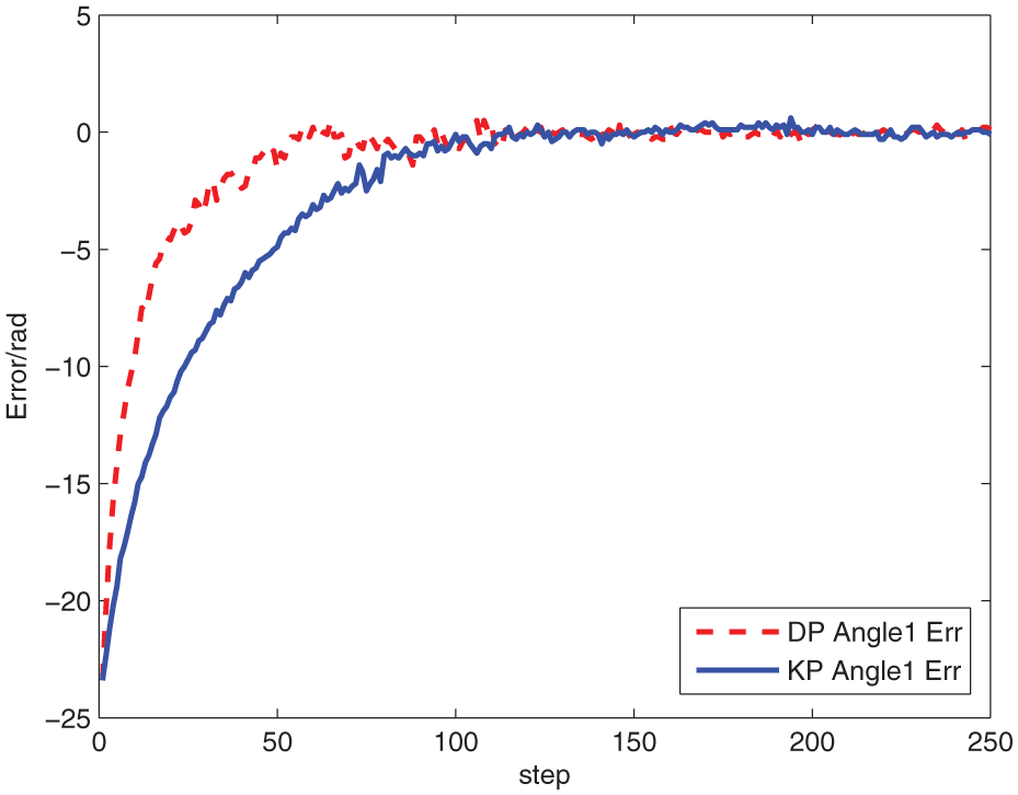
Angle error’s contrast curve in camera 1.

Figure 17.

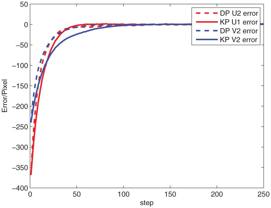
Point error’s contrast curve in camera 2.

Figure 18.

Angle error’s contrast curve in camera 2.

According to the comparison of experiment data, the image feature error in the image plane is within 1 pixel or degree and the posture error in the Cartesian space is less than 1 mm or 1° under any of the two methods. Figure 19 shows the two methods’ error contrast curve in the Cartesian space, as well as Figure 20 indicates the contrast trajectory of the robot manipulator in the Cartesian space. Therefore, the effectiveness of the two methods has little difference. But the image Jacobian matrix method requires real-time to estimate the image Jacobian matrix and to calculate the inverse of the image Jacobian matrix. Thus, the disadvantage of this method is the calculation of the complex matrix and the irreversible of the image Jacobian matrix. For comparison, the proposed method can completely avoid complex mathematical operations and the irreversible of matrix.

Figure 19.

Posture error curve in Cartesian space.

Figure 20.

Point contrast curve in Cartesian space.

Conclusion

In this article, the two-camera bi-axial parallel vision configuration was proposed to realize robot manipulator uncalibrated visual serving. The qualitative mathematical model was established under the proposed vision configuration, and the relationship between the feature point and line in the Cartesian space and the corresponding point and angle in the image space has been analyzed. Then, the controller was designed by selecting the specific feature point and line in the image plane. By taking the nonlinear dynamic forces of the robot manipulator into account, the Lyapunov theory was used to prove that the robot manipulator can achieve global asymptotic stability in the Cartesian space. Finally, the simulation and physical experiments realized the robot manipulator five-degrees of freedom uncalibrated vision positioning, and the experimental results verify the validity of the proposed control method and vision configuration.