Sage Journals: Discover world-class research

Abstract

The constant-frequency double-rotor generator has the potential to be used in the marine energy conversions, such as tides and marine current power generation system due to the advantages. However, there are two different rotational speed movement boundaries in the constant-frequency double-rotor generator, especially the inner moving part boundary between the inner wound rotor and outer permanent magnet rotor. This complicates the finite element analysis and greatly increases the analysis time. In this article, a new finite element analysis method based on double boundaries interpolation multiple reference frame is proposed. The principle of the interpolation multiple reference frame method is introduced, and the analysis and comparison with the traditional method are carried out. The analysis results show that the interpolation multiple reference frame method simplifies the preprocessing procedure, reduces computation time, ensures high calculation accuracy, and has the potential to be applied in all kinds of multiple mechanical port machines.

Keywords

Double-rotor generator marine energy electromagnetic field analysis time-stepping finite element method

Introduction

The constant-frequency double-rotor (CFDR) generator is a kind of variable-speed constant-frequency (VSCF) generator, which may be used in the application of ocean energy harvesting.¹ The CFDR generator outputs a fixed frequency electrical power, so it can be directly integrated with the grid.^2,3 The CFDR generator has the advantages of no gearbox, high efficiency, and flexible regulation of active and reactive power. Then the CFDR generator is very suitable for large-scale conversion of marine energy.

The finite element method (FEM) is one of the most commonly used methods in electrical machine design and analysis. The static as well as the transient FEM are commonly used to analyze the performance of the electric machine. The time-stepping FEM based on field-circuit-mechanical equation coupling is one of the most effective transient FEMs. In electrical machines, there is a relative movement between the stator and rotor. The meshing must be executed in every step of the finite element analysis, which will take a lot of computing time. And the shape of the new mesh will be distorted, which may lead to reduced calculation accuracy. Hence, how to deal with the motion problem of the electrical machine is very important.

In previous literatures, there are several effective methods to treat the movement of the electrical machines. The conception of an air-gap element for the dynamic analysis of the electromagnetic field in electric machines is proposed in Abdel-Razek et al.⁴ In this air-gap element method, the entire air-gap region is one macro element and its field is calculated analytically using a Fourier series expansion of the vector potential. The movement is accomplished by a simple recalculation of the Fourier series without any modification of the mesh structure, resulting in simple and efficient time-stepping.^5–7 The results can be very accurate because of the high order of the field representation in the air-gap region.⁸ But for the insertion of dense matrix blocks into the sparse finite element matrices, the computational time is substantially increased.^9,10 The moving band method is proposed in Davat et al.¹¹ There is no need of the special elements or coupling techniques; no dense blocks are generated in the system matrix and the system dimension is not increased.¹² For this reason, the moving band method should be superior to the air-gap element method in terms of computational speed. However, re-meshing the air-gap region is inevitable, and thus the numbering as well as the amount of nodes in the mesh are not constant. The conditioning of the system matrix is not maintained and preprocessing must be rerun when the mesh changes. Also, because the elements in the air-gap are geometrically distorted or re-meshed to accommodate arbitrary movement, the results often have an oscillating error component.⁵ It has been shown that this problem can be drastically reduced by using higher order elements in the moving band.¹³ However, the use of higher order elements increases the density of the element, and the computational time will substantial increase as the case of the air-gap element method.

A hybrid finite element–boundary integral method is proposed in Salon and Schneider.¹⁴ Using this method, users can represent any region by either finite elements or boundary elements. There are many advantages, such as the number of equations can be reduced by using boundary, open boundary problems are easily formulated, and non-linear regions can be represented by finite elements.¹⁵ However, this method increases the bandwidth of the system matrix and increases the computational time. An interpolation slip surface method is proposed in Yan et al.¹⁶ It effectively treats the single movement boundary. But for the multiple mechanical port machines, there are different speed movement boundaries, which complicate the preprocessing procedure and increase the analysis time. In this article, a new finite element analysis method based on double boundaries interpolation multiple reference frame (DBIMRF) method suitable for the CFDR generator is proposed. The proposed method simplifies the preprocessing procedure, reduces computation time, ensures high calculation accuracy, and has the potential to be applied in all kinds of multiple mechanical port machines. The DBIMRF method could be implemented in ANSYS by ANSYS Parametric Design Language. Through the combination of the IMRF method and ANSYS, the simulation time may be greatly decreased.

DBIMRF method

During the design of the electrical machines, the simplest way to analyze the static electromagnetic field is re-meshing the machine domain in every step of the movement, and it can obtain the most accurate calculation result. However, this may greatly increase the simulation time. The moving band method is commonly used in the transient electromagnetic field simulation, which only needs re-meshing the air-gap between the rotor and the stator in every step, so that it can reduce the simulation time, but the re-meshing will produce distorted elements and the distorted element will lead to the calculation accuracy decreasing.

The slip surface method

The slip surface method is proposed in Yan et al.¹⁶ It does not need to re-mesh and would not change the shape of the element. So it ensures the calculation accuracy, greatly reduces the simulation time, and it is easy to realize.¹⁷

The theory of the slip surface method is as follows. First, two independent coordinate systems, namely, a static coordinate system and a rotating coordinate system, are used for the stator and the rotor, respectively. Second, the electromagnetic field equations of the stator and the rotor are set up, respectively. Then the equations of stationary parts and rotating parts are solved in parallel through the movement boundary condition. Finally, the whole field solution can be obtained. The specific implementation tips are presented as shown in Figure 1.

Figure 1.

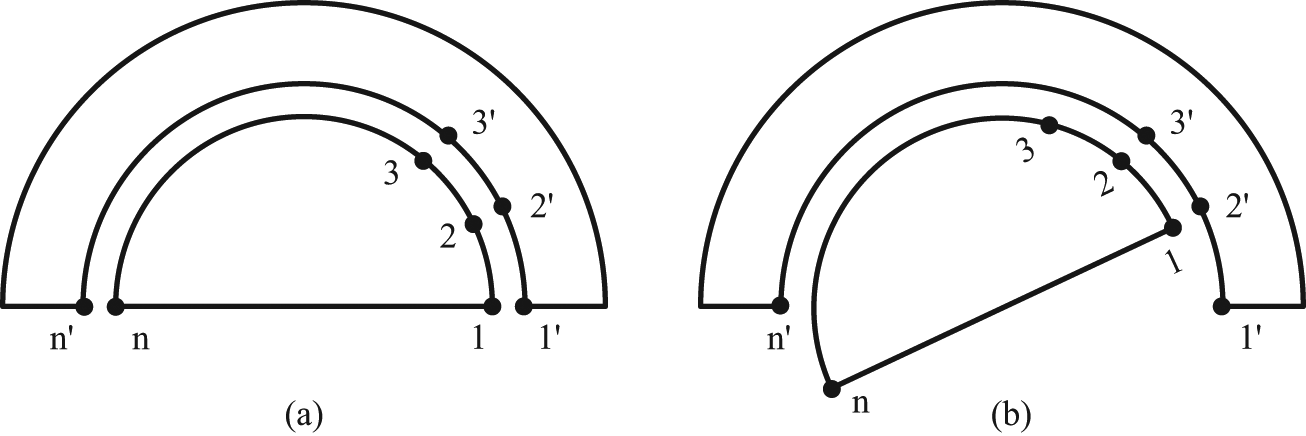
Specific implementation tips of slip surface method.

As shown in Figure 1, a movement boundary that consists of two overlapping arcs belonging to the stator and the rotor, respectively, is set up inside the air-gap between the stator and the rotor. There are n equidistant nodes on each arc, and each arc is divided into n − 1 segments. In the initial position, the nodes on the two arcs coincide. The radian of each curve segment or its integral multiple is equal to the rotor rotation step size. So the nodes belonging to the stator and the rotor on the movement boundary are overlapped in every step and the meshes of the stator and the rotor do not need to be changed.

The slip surface method can reduce computation time and ensure high calculation accuracy. In the design of the CFDR generator, this method can improve the efficiency and accuracy very well, but for the transient performance simulation, it is not suitable.

Figure 2 shows the structure of the CFDR generator. It consists of three parts: wound stator, inner wound rotor, and outer permanent magnet (PM) rotor. The freely rotating outer rotor is located between the stator and the inner rotor. There are two air-gaps and two movement boundaries in CFDR generator where the inner movement boundary is between two rotating parts. For the different rotational speed of two movement boundaries, the time step size is not easy to determine. The nodes on the boundaries of slip surface method might be too dense in analyzing the CFDR generator. It will lead to longer calculation time, lower calculation accuracy, and even not convergence. So the slip surface method must be improved for the analysis of CFDR generator.

Figure 2.

Structure of CFDR generator.

The DBIMRF method

The first-order linear triangle-shaped element is selected in the finite element model. The triangle-shaped element has six nodes, as shown in Figure 3. The vector magnetic potential (A_Z) of the node m is equal to (A_Zi + A_Zk)/2. According to the principle of finite element, the A_Z of the point on the side of element satisfies linear equation, and the A_Z of node on the movement boundary can be similar to the A_Z of the point on the side of element. So the Lagrangian interpolation method can be used to deal with the movement boundary and do not need to request the space step length and node distance matching.

Figure 3.

Triangle-shaped element.

Figure 4 shows that there are two movement boundaries, L₁ and L₂. For the existence of L₂ which is between two rotating parts, the difficulty of dealing with the boundary problem is increased. In order to reduce the complexity and difficulty of programming, improve the portability of the program; double boundaries method is used.

Figure 4.

Movement boundaries and boundary conditions of CFDR generator.

The implementation of DBIMRF method is as follows. Three independent coordinate systems, namely, the Euler coordinate system (static coordinate system) and two Lagrangian coordinate systems (servo) are set up for the stator, inner rotor, and outer rotor, respectively. The magnetic fields of the three parts are solved, respectively. And the magnetic fields are coupled through the vector magnetic potential (A_Z) of the nodes on the movement boundaries. The nodes, boundary conditions, and movement boundaries of the CFDR generator in the IMRF method are shown in Figure 4. The moving boundary L₁ is composed of two overlapping circular arcs, which belong to the stator and the rotor, respectively. Lagrange interpolation coupling method is used to couple A_Z of the nodes by periodic boundary condition, as

{\begin{matrix} A_{ZK} = K_{1} A_{Z (j + 1)} + K_{2} A_{Z} \\ K_{1} = \frac{θ_{j, k}}{θ_{j, j + 1}}, K_{2} = \frac{θ_{k, j + 1}}{θ_{j, j + 1}} \end{matrix}

(1)

where K₁ and K₂ are the Lagrangian interpolation coefficient. So it is easy in preprocessing where the space step length has no relationship with the node distance.

Not same as L₁, the boundary L₂ between the outer and the inner rotor is not treated as the active boundary. Using double moving boundary method, two movement boundaries, L₃ and L₄, are defined. Then the air-gap between the outer and the inner rotor is divided into three parts. The part between L₃ and L₄ is treated as a static part where the boundary of the moving part and the static part is realized. In this case, L₃ and L₄ may be treated in the way as L₁. Using this method, the finite element preprocessing procedure is greatly simplified.

The DBIMRF method is the improvement of the slip surface method in the application of the transient electromagnetic field analysis. The distance between the nodes is determined by the space step length as the CFDR generator running in the steady state. So the high accuracy of the CFDR static performance analysis and the effectiveness of transient performance analysis all may be achieved.

Element stiffness matrix

The shape and size of the element are not changed in every step by using the DBIMRF method. Because the shape and size of the element are not changed, the element stiffness matrix will not be changed. So the calculation accuracy will not be reduced and it can be proved as follows.

Figure 3 shows that the numbers of three vertices of the triangle-shaped element are i, j, and k, which are arranged in counterclockwise direction. And their coordinates are (x_i, y_i), (x_j, y_j), and (x_k, y_k), respectively. The side lengths of the three sides are l_i, l_j, and l_k, respectively

{\begin{matrix} a_{i} = x_{k} - x_{j} = Δ x_{kj} \\ a_{j} = x_{i} - x_{k} = Δ x_{ik} \\ a_{k} = x_{j} - x_{i} = Δ x_{ji} \end{matrix}

(2)

{\begin{matrix} b_{i} = y_{j} - y_{k} = Δ y_{jk} = - Δ y_{kj} \\ b_{j} = y_{k} - y_{i} = Δ y_{ki} = - Δ y_{ik} \\ b_{k} = y_{i} - y_{j} = Δ y_{ij} = - Δ y_{ji} \end{matrix}

(3)

K_{st} = \frac{1}{4 μ S_{e}} (a_{s} a_{t} + b_{s} b_{t}), s, t = i, j, k

(4)

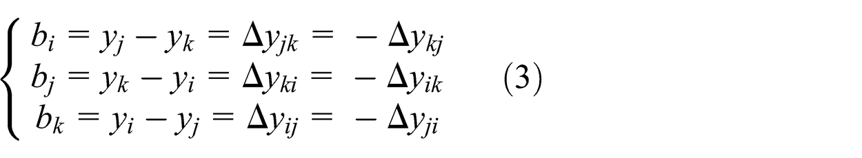
where S_e is the area of the element and µ is the permeability of the element material. Then the element stiffness matrix can be obtained as equation (5)

K = [\begin{matrix} K_{ii} & K_{ij} & K_{ik} \\ K_{ji} & K_{jj} & K_{jk} \\ K_{ki} & K_{kj} & K_{kk} \end{matrix}]

(5)

K_{ss} = \frac{1}{4 μ S_{e}} (a_{s}^{2} + b_{s}^{2}) = \frac{1}{4 μ S_{e}} l_{s}^{2} s, s = i, j, k

(6)

\begin{matrix} K_{ji} = K_{ij} = \frac{1}{4 μ S_{e}} (a_{s} a_{t} + b_{s} b_{t}) \\ = \frac{1}{4 μ S_{e}} (Δ x_{kj} Δ x_{ik} + Δ y_{kj} Δ y_{ik}) \\ = \frac{1}{4 μ S_{e}} (\frac{{(Δ x_{kj} + Δ x_{ik})}^{2} - Δ x_{kj}^{2} - Δ x_{ik}^{2}}{2} \\ + \frac{{(Δ y_{kj} + Δ y_{ik})}^{2} - Δ y_{kj}^{2} - Δ y_{ik}^{2}}{2}) \\ = \frac{1}{4 μ S_{e}} (\frac{Δ x_{ij}^{2} - Δ x_{kj}^{2} - Δ x_{ik}^{2}}{2} + \frac{Δ y_{ij}^{2} - Δ y_{kj}^{2} - Δ y_{ik}^{2}}{2}) \\ = \frac{1}{8 μ S_{e}} (l_{k}^{2} - l_{i}^{2} - l_{j}^{2}) \end{matrix}

(7)

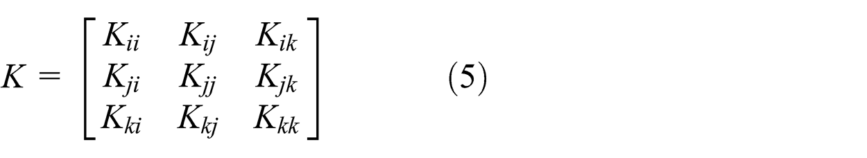
Similarly, the other elements of the element stiffness matrix can be obtained

K_{ik} = K_{ki} = \frac{1}{8 μ S_{e}} (l_{j}^{2} - l_{k}^{2} - l_{i}^{2})

(8)

K_{jk} = K_{kj} = \frac{1}{8 μ S_{e}} (l_{i}^{2} - l_{j}^{2} - l_{k}^{2})

(9)

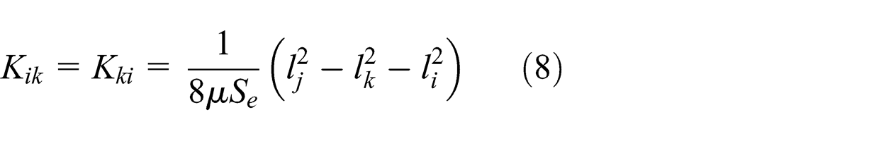
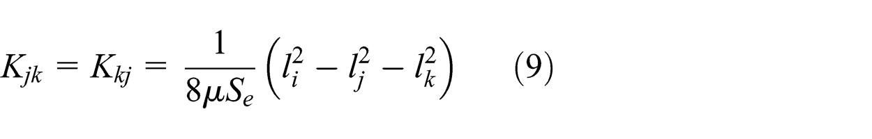
From equations (6)–(9), it can be seen that the element stiffness matrix is only dependent on the shape and size of the element, no matter with the position and rotation angle of the element. So, using the slip surface and DBIMRF method, the element stiffness matrix will not be changed in every step. So the global stiff matrix will not be changed and the high calculation accuracy can be achieved.

Electromagnetic field analysis

The static electromagnetic field analysis

In order to verify the effectiveness of DBIMRF method, the IMRF method in static electromagnetic field simulation is used for analyzing a specific CFDR generator model. The main dimensions of the CFDR generator are shown in Table 1. Considering the symmetry of CFDR generator structure, the geometrical model of half CFDR generator is established as shown in Figure 5, where the material properties are displayed by different colors.

Table 1.

The main dimensions of the CFDR generator.

Item	Stator	Outer PM rotor	Inner rotor
OD (mm)	210	153.2	132.2
ID (mm)	154.4	133.2	41

OD: outer diameter; ID: inner diameter.

Figure 5.

Geometrical model of CFDR generator.

The accuracy of FEM largely depends on the level of meshing. For achieving high accuracy calculation, high level of meshing for the CFDR generator is adopted, as shown in Figure 6. Then, according to Figure 4, the boundary conditions are implemented on the finite element model, as shown in Figure 7.

Figure 6.

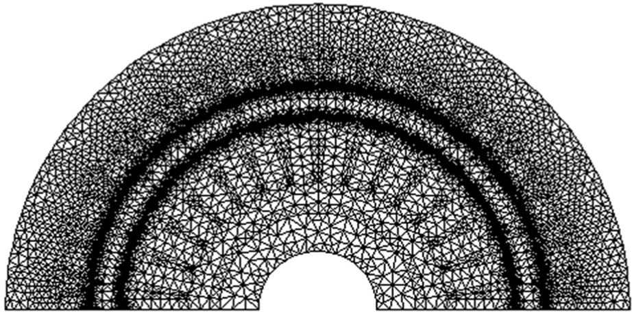
Mesh model of CFDR generator.

Figure 7.

Finite element model of CFDR generator with boundary conditions.

The flux distributions and magnetic flux density of the CFDR generator only under PM excitation are shown in Figure 8. It is shown that most of the PM flux goes through the stator and inner rotor; meanwhile, the magnetic field of the corresponding stator and rotor tooth is saturated, and the excitation of the generator is provided by the PM. The result is consistent with the actual situation.

Figure 8.

Magnetic field of CFDR generator: (a) magnetic flux distribution in CFDR generator and (b) magnetic flux density in CFDR generator.

The calculation accuracy and time of the IMRF method are studied and compared with the re-meshing method. The same number and shape of element are selected. Here, the number of the element is 48,363. For comparing fairly, two methods are carried out on the same computer, which has a configuration as shown in Table 2.

Table 2.

Computer configuration.

CPU	Operating system	Memory	Primary hard drive
Intel(R) Core(TM) i5-2400 at 3.10 Hz	Windows 7 UltimateSP1 64Bit	4GB KingstonDDR31333 MHz	1TB/7500 r/min Western Digital Corp

The un-alignment of boundary nodes may influence the calculation accuracy of the IMRF method. In order to analyze calculation accuracy of the IMRF method in the disadvantage conditions, the rotor rotation angle is set not equal to the integer times of node spacing. In the static electromagnetic field analysis, only the no-load electromotive force (EMF) of the inner rotor is studied. So the inner rotor is seen as a static part, and only the outer rotor rotates. Using the IMRF method and the re-meshing method, the no-load EMF at rated speed can be obtained, respectively. Figure 9 shows the no-load EMF waveforms of phase A winding of the inner rotor. It can be seen that the result agrees very well. Figure 10 shows the relative error caused by the DBIMRF method. The relative error is calculated based on the result of the re-meshing method as truth value. According to Figure 10, it can be seen that the impact caused by nodes un-alignment is very small and can be ignored in the DBIMRF method. So the IMRF method can keep the high calculation accuracy.

Figure 9.

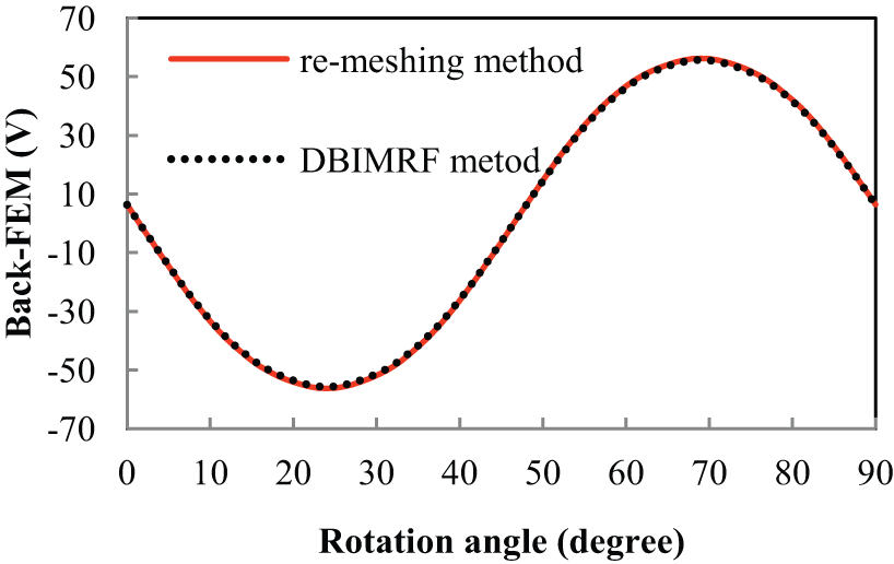
No-load EMF of phase A winding of the inner rotor.

Figure 10.

Relative error caused by the double boundaries IMRF method.

There are 90 steps which are set up in analysis, and the calculation times by using IMRF method and re-meshing method are 42.5 and 68 min, respectively. It is shown that the DBIMRF method may greatly reduce the calculation time. And with the step number increasing, the proportion of the saved time will be increased.

Time-stepping FEM simulation

In this section, the DBIMRF method is used in the time-stepping FEM to analysis the no-load start-up process of the CFDR generator. The electromagnetic field and the mechanical movement equation should be coupled during the calculation. There are two coupling methods: direct coupling method and indirect coupling method.^18,19 The direct method directly plugs the angular velocity into the electromagnetic field finite element equation (10), which will result in asymmetrical matrix and lead to the difficulty of solving finite element equations. So the indirect coupling method is adopted in this article

\nabla \times (\frac{1}{μ} \nabla \times A) + σ (\frac{\partial A}{\partial t} - V \times (\nabla \times A)) = J

(10)

where µ is the reluctivity, A is the magnetic vector potential, V is the velocity, and J is the current density in the coils.

The basic idea of indirect coupling method is as follows. The position of the rotor at kth step is replaced by the position of the rotor at (k − 1)th step. The coefficient matrix of the field-circuit coupling finite element equations will keep constant during the solution. After the kth step calculation of the electromagnetic field is finished, the torque can be obtained and the rotor position of kth step will be obtained by combining the rotor mechanical motion equation. Then the continued calculation of (k+1)th step might be carried out in the same way. By this method, the solution of the field-circuit-mechanical motion coupled equations will be obtained.

The mechanical motion equation of the outer PM rotor is

{\begin{matrix} J_{m} \frac{d Ω}{dt} = T_{em} - T_{L} \\ Ω = \frac{d θ}{dt} \end{matrix}

(11)

where the Ω is the rotating speed of the outer PM rotor, θ is the position of the PM rotor, J_m is the rotational inertia of the PM rotor, T_em is the electromagnetic torque, and T_L is the load torque.

When the space step size Δθ is fixed, forward-difference (explicit Euler method) is used for the discretization of the mechanical motion equation (12). Assuming that the rotor rotates at a constant velocity in every step, the mechanical motion equation is

{\begin{matrix} Ω^{(n)} = Ω^{(n - 1)} + \frac{T_{em}^{(n - 1)} - T_{L}}{J_{m}} Δ t^{(n - 1)} \\ Δ t^{(n)} = \frac{Δ θ}{Ω^{(n)}} \end{matrix}

(12)

Fixed space step size is suitable for slip surface method, but it is not suitable for analyzing the start-up process of CFDR generator, since the generator runs in a wide range of speed. The transient process in a short time is concerned in transient analysis, and the fixed space step size limited the time step, that is inconvenient.

When the time step size is fixed, backward-difference (implicit Euler method) is used for the discretization of the mechanical motion equation (11). Assuming that the rotor rotates as uniformly accelerated motion in every step, the mechanical motion equation can be expressed as

{\begin{matrix} Ω^{(n)} = Ω^{(n - 1)} + \frac{T_{em}^{(n)} - T_{L}}{J_{m}} Δ t \\ Δ θ^{(n)} = Ω^{(n)} Δ t + \frac{1}{2} \frac{T_{em}^{(n)} - T_{L}}{J_{m}} Δ t^{2} \end{matrix}

(13)

After knowing the electromagnetic torque, the current speed Ω⁽ⁿ⁾ can be calculated by equation (13), and then the Δθ⁽ⁿ⁾, which is the space step size of the next step, can be obtained. The position of the rotor can also be calculated. Through this method, the dynamic change in electromagnetic torque and current of the CFDR generator may be calculated.

The DBIMRF method adopts the fixed time step size, which overcomes the difficulty in selection of the time step size and does not cause any increase in the calculation time and the complexity of the pre-treatment procedure. This effectively guarantees the calculation accuracy. The analysis result of the CFDR generator start-up process is shown in Figure 11. For verifying correctness of the result, the result is compared with high-order moving band method, which has been proved highly accurate. It can be seen from Figure 11 that the accuracies of the two methods are closing. So the IMRF method guarantees the calculation accuracy. And according to Figure 11, the transient stability of the CFDR generator is well where the speed, torque, and current only have slight perturbation around the ideal value. The CFDR generator has the potential to be applied in ocean energy harvesting.

Figure 11.

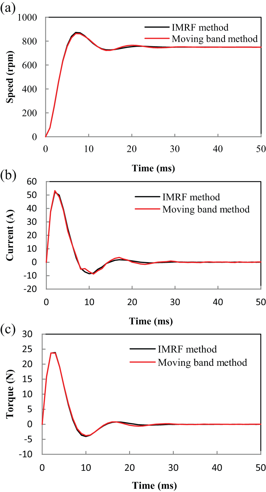
Analysis result of start-up process: (a) out rotor speed, (b) inner rotor current, and (c) torque.

Conclusion

The CFDR generator has two rotors with different rotation speeds and brings difficulties to the electromagnetic field finite element analysis. To deal with this problem, a DBIMRF method is introduced and studied in this article. Due to cancellation of the constraint that the nodes on the movement boundaries must be constantly overlapped, a fixed time step size is adopted without considering the space step size. The space step size is obtained by calculation. It is verified that the method solves the difficulty in choosing the time step without increasing the density of the elements, greatly shortens the calculation time, and effectively guarantees the calculation accuracy.

Footnotes

Academic Editor: Fabrizio Marignetti

Declaration of conflicting interests

The authors declare that they have no conflict of interest.

Funding

This work was supported, in part, by the National Key Basic Research Program of China (973 Program of China) (2013CB035603) and the National Natural Science Foundation of China (51137001, 51320105002).

References

Zhang

Cheng

Zhu

. A constant-frequency double-rotor generator for wind power application. In: 2010 International conference on electrical machines and systems (ICEMS), Incheon, South Korea, 10–13 October 2010, pp.583–587. New York: IEEE.

Thresher

. A commercialization path and challenges for marine hydrokinetic renewable energy. In: 2011 IEEE power and energy society general meeting, San Diego, CA, 24–29 July 2011, pp.1–8. New York: IEEE.

Santos-Mugica

Robles

Endegnanew

. Grid integration and power quality testing of Marine Energy Converters: research activities in the MARINET project. In: 2014 Ninth international conference on ecological vehicles and renewable energies (EVER), Monte-Carlo, 25–27 March 2014, pp.1–9. New York: IEEE.

Abdel-Razek

Coulomb

Feliachi

. Conception of an air-gap element for the dynamic analysis of the electromagnetic field in electric machines. IEEE Trans Magn 1982; 18(2): 655–659.

Silwal

Rasilo

Perkkio

. Evaluation and comparison of different numerical computation methods for the electromagnetic torque in electrical machines. In: 2013 International conference on electrical machines and systems (ICEMS), Busan, South Korea, 26–29 October 2013, pp.837–842. New York: IEEE.

De Gersem

Weiland

. Reformulation and generalisation of the air-gap element. International COMPUMAG Society Newsletter (ICS) 2005; 12(1): 2–8.

De Gersem

Weiland

. A computationally efficient air-gap element for 2D FE machine models. IEEE Trans Magn 2005; 41(5): 1844–1847.

Aliprantis

. Optimal design of electromechanical devices using a hybrid finite element/air-gap element method. In: IEEE power and energy conference at Illinois (PECI), Champaign, IL, 22–23 February 2013, pp.106–113. New York: IEEE.

Flack

Volschenk

. Computational aspects of time-stepping finite element analysis using an air-gap element. In: Proceedings of the international conference on electrical machines, Paris, France, September 1994, pp.158–163. Paris: Comite d’ICEM–94.

10.

Lee

DeBortoli

Lee

. Coupling finite elements and analytical solution in the air gap of electrical machines. IEEE Trans Magn 1991; 27(5): 3955–3957.

11.

Davat

Ren

Lajoie-Mazenc

. The movement in field modeling. IEEE Trans Magn 1985; 21(6): 2296–2298.

12.

Dular

Geuzaine

Ferreira

Luz

. Connection boundary conditions with different types of finite elements applied to periodicity conditions and to the moving band. COMPEL 2001; 20(1): 109–119.

13.

Rodger

Lai

Leonard

. Coupled elements for problems involving movement. IEEE Trans Magn 1990; 26(2): 548–550.

14.

Salon

Schneider

. A hybrid finite element-boundary integral formulation of Poisson’s equation. IEEE Trans Magn 1981; 17(6): 2574–2576.

15.

Sadowski

Lefevre

Lajoie-Mazenc

. Finite element torque calculation in electrical machines while considering the movement. IEEE Tras Magn 1992; 28(2): 1410–1413.

16.

Yan

Liu

. A new method to deal with the motion problem in electromagnetic field finite element analysis. Proc CSEE 2003; 23(8): 163–167.

17.

Preston

Reece

ABJ

Sangha

. Induction motor analysis by time-stepping techniques. IEEE Trans Magn 1988; 24(1): 471–474.

18.

Bedrosian

. A new method for coupling finite element field solutions with external circuits and kinematics. IEEE Trans Magn 1993; 29: 1664–1668.

19.

. A novel approach to circuit-field-torque coupled time stepping finite element modeling of electric machines. IEEE Trans Magn 2000; 36(4): 1886–1889.

The treatment of moving problem for constant-frequency double-rotor generator in finite element analysis