
Abstract
Lattice Boltzmann method combined with large eddy simulation is developed in the article to simulate fluid flow at high Reynolds numbers. A subgrid model is used as a large eddy simulation model in the numerical simulation for high Reynolds flow. The idea of subgrid model is based on an assumption to include the physical effects that the unresolved motion has on the resolved fluid motion. It takes a simple form of eddy viscosity models for the Reynolds stress. Lift and drag evaluation in the lattice Boltzmann equation takes momentum-exchange method for curved body surface. First of all, the present numerical method is validated at low Reynolds numbers. Second, the developed lattice Boltzmann method/large eddy simulation method is performed to solve flow problems at high Reynolds numbers. Some detailed quantitative comparisons are implemented to show the effectiveness of the present method. It is demonstrated that lattice Boltzmann method combined with large eddy simulation model can efficiently simulate high Reynolds numbers’ flows.
Introduction
Recently, the lattice Boltzmann method (LBM) has emerged as a well-known alternative of computational technique in fluid dynamics for modeling fluid flow in a way that is consistent with the Navier–Stokes equation,1,2 due to its intrinsic advantages over conventional Navier–Stokes schemes. The LBM is an innovative numerical method based on kinetic theory to simulate various hydrodynamic systems; it is a reasonable candidate for simulation of turbulence, flow-induced noise, and sound propagation.
The development of the lattice Boltzmann equation (LBE) was independent of the continuous Boltzmann equation. It was introduced to solve some of the difficulties of the lattice gas automata (LGA). A parameter matching procedure based on the Chapman–Enskog analysis of the LGA needs to construct a set of relaxation equations so that the correct hydrodynamic equations are derived.
Compared to the second-order Navier–Stokes equations, the LBM is derived from a set of first-order partial differential equations the LBM formulation does not include nonlinear convection term while Navier–Stokes solvers have to treat such nonlinear one. Moreover, it is necessary for the incompressible Navier–Stokes equations to solve the Poisson’s equation, and then the pressure can be obtained. However, the pressure in the LBM is determined directly from the state equation; the computing cost can be decreased. Furthermore, it has been shown that complex boundary geometries are treated easily in LBM. As a result, LBM has widely emerged as a computational tool for practical engineering applications in the simulations of fluid flows3,4 and aerospace industries. 5
It is well known that the LBM is often used as a direct numerical simulation tool without any assumptions for the relationship between the turbulence stress tensor and the mean strain tensor. Thus, the smallest captured scale in the LBM is the lattice unit, and the largest scale depends on the characteristic length scale in the simulation. These scales are often determined by the available computer memory. Consequently, the LBM is able to resolve relatively low Reynolds number flows. Numerical studies 6 have shown that LBM can result in the numerical instability for simulating high Reynolds number flows if unresolved small-scale effects on large-scale dynamics are not considered. A better option is to combine the LBM and large eddy simulation (LES) model in order to solve the problem at high Reynolds numbers. A subgrid model is often used as an LES model in the numerical simulation for traditional Navier–Stokes equation. The idea of subgrid model 7 is based on an assumption to include the physical effects that the unresolved motion has on the resolved fluid motion. The model often takes a simple form of eddy viscosity models for the Reynolds stress.
Smagorinsky model 7 is one of all subgrid models, including the standard Smagorinsky model and dynamic subgrid model. The standard Smagorinsky model uses a positive eddy viscosity to represent small-scale energy damping. Nevertheless, the shortcoming of the standard one is that the eddy viscosity could be large and positive at some scales smaller than test grids, while it can be large and negative at others sometimes. 7 Compared with the standard one, dynamic subgrid models 8 could include the dependence of the subgrid model coefficients on local quantities to overcome these side effects.
LBM
The governing equation of LBM for describing fluid flows is Boltzmann equation modeled by adopting the Bhatnagar, Gross, and Krook 9 (BGK) collision model. In contrast to the traditional schemes of solving the discretized Navier–Stokes equations, LBM approach focuses on the microscopic scales via the discrete Boltzmann equation and tracks particle distributions on a lattice. The standard LBE involving BGK model can be written into the following form
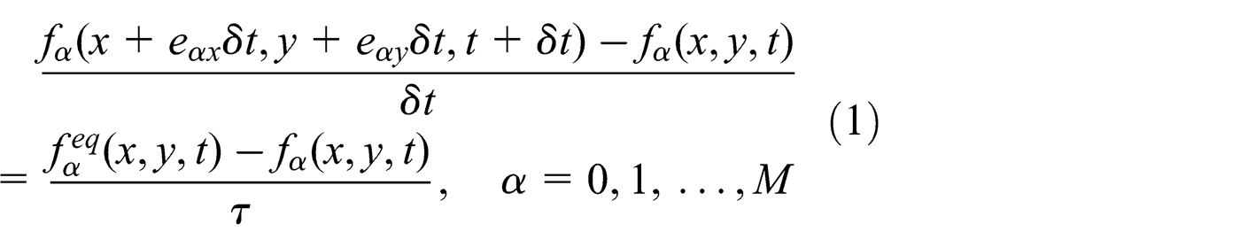
where

The macroscopic quantities, density and momentum density, can be obtained directly from the distribution function

The pressure
In the simulation, the particle velocity model D2Q9
10
is used in the present code. The discrete velocity set


For the treatment of boundary condition, Zou and He’s 11 non-equilibrium bounce-back scheme is applied on the far-field boundary in the computational domain due to its second-order accuracy. The boundary condition for the particle distribution functions on the curved wall is handled with second-order accuracy based on Mei et al.’s 12 work. Lift and drag evaluation in the LBE takes momentum-exchange method for curved boundary. Mei has shown that it is reliable, accurate, and easy to implement for both two-dimensional and three-dimensional flows.
Subgrid model for LES
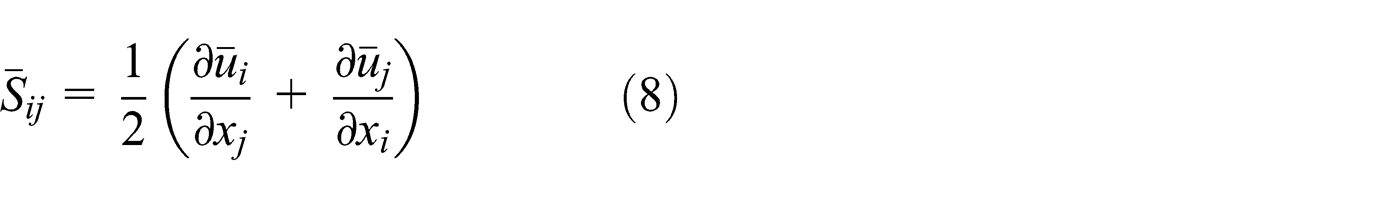
In the LES, the most common subgrid model is the Smagorinsky one, where the anisotropic part of the Reynolds stress term is modeled as

in which
Next, LBM is modified to simulate the filtered physical variables in the LBE. First, the filtered particle distribution

Then the LBE can be written into a kinetic equation for the filtered particle distribution function

The above equation for
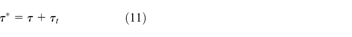
Then the total viscosity can be denoted as follows

where
Numerical results
Circular cylinder in low Reynolds numbers’ flow
To validate the program developed in the article, low Reynolds numbers’ flow around a circular cylinder is first simulated here. As depicted in Figure 1, the fluid with the velocity
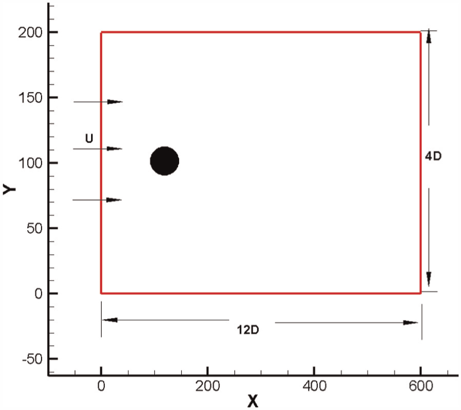
Computational domain.

Computational mesh.
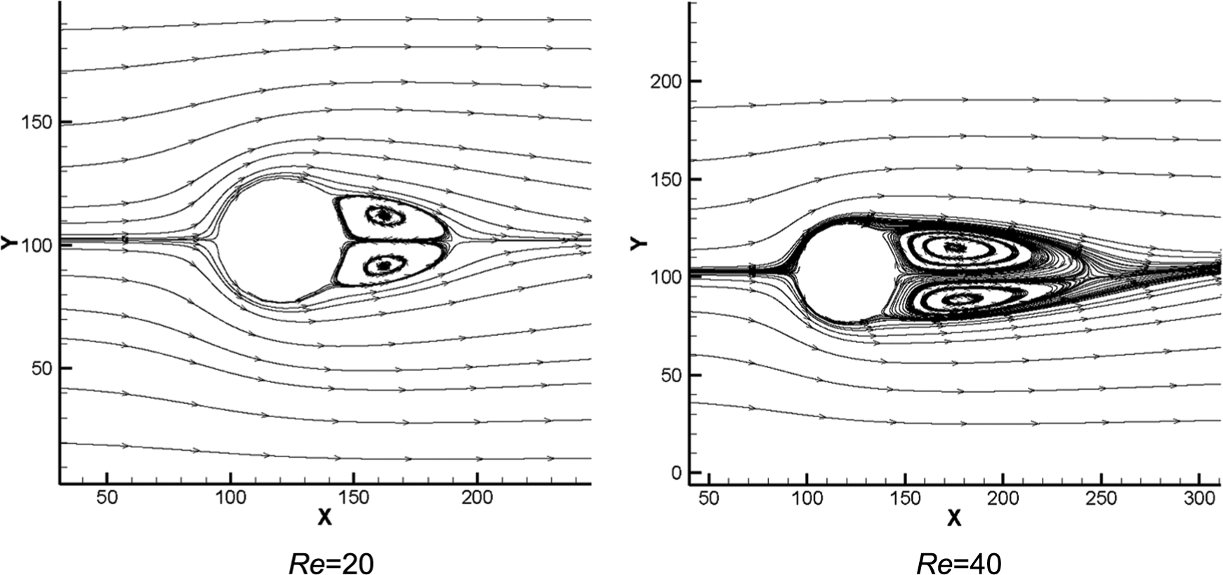
Stream line for Re = 20 and 40.

Vortex contours for cylinder.
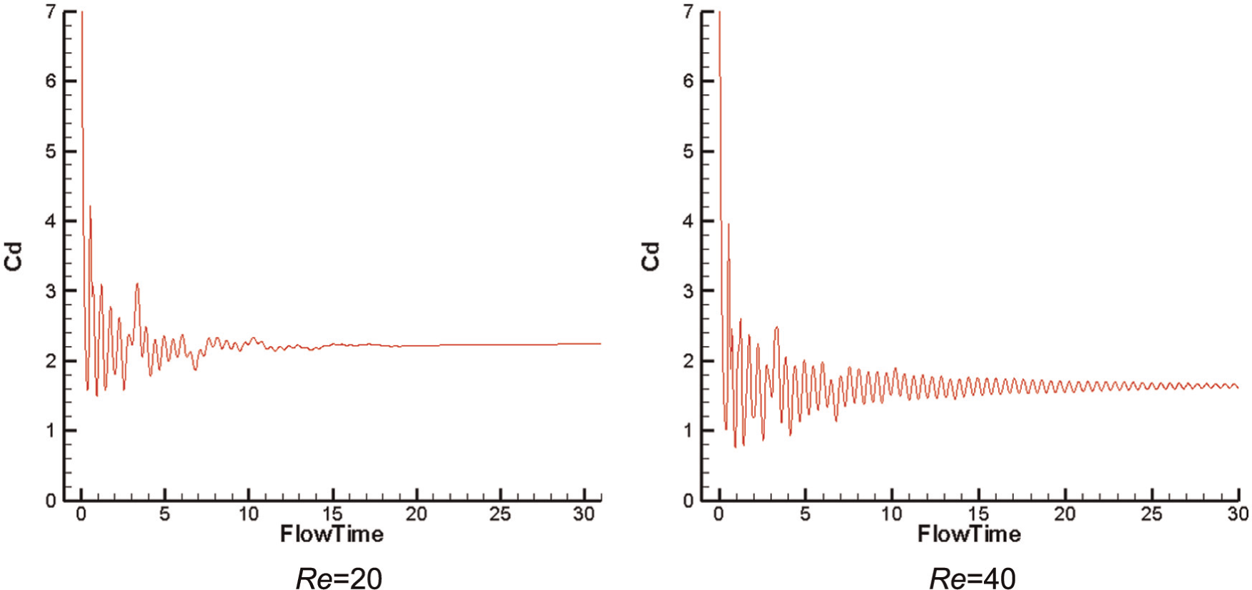
Time history of Cd for cylinder.
Comparisons of lift and drag.

Lid-driven cavity flow at high Reynolds numbers
Lid-driven cavity flow is considered here to validate the simulation for high Reynolds flow using the present developed LBM/LES model. It is a classic problem for studying the complex flow in a simple geometry. As shown in Figure 6, flow is driven by the uniform velocity U on the top boundary of square cavity; vortex will be formed inside the cavity depending on the different Reynolds number Re. A uniform grid is used in the present simulation in Figure 6.
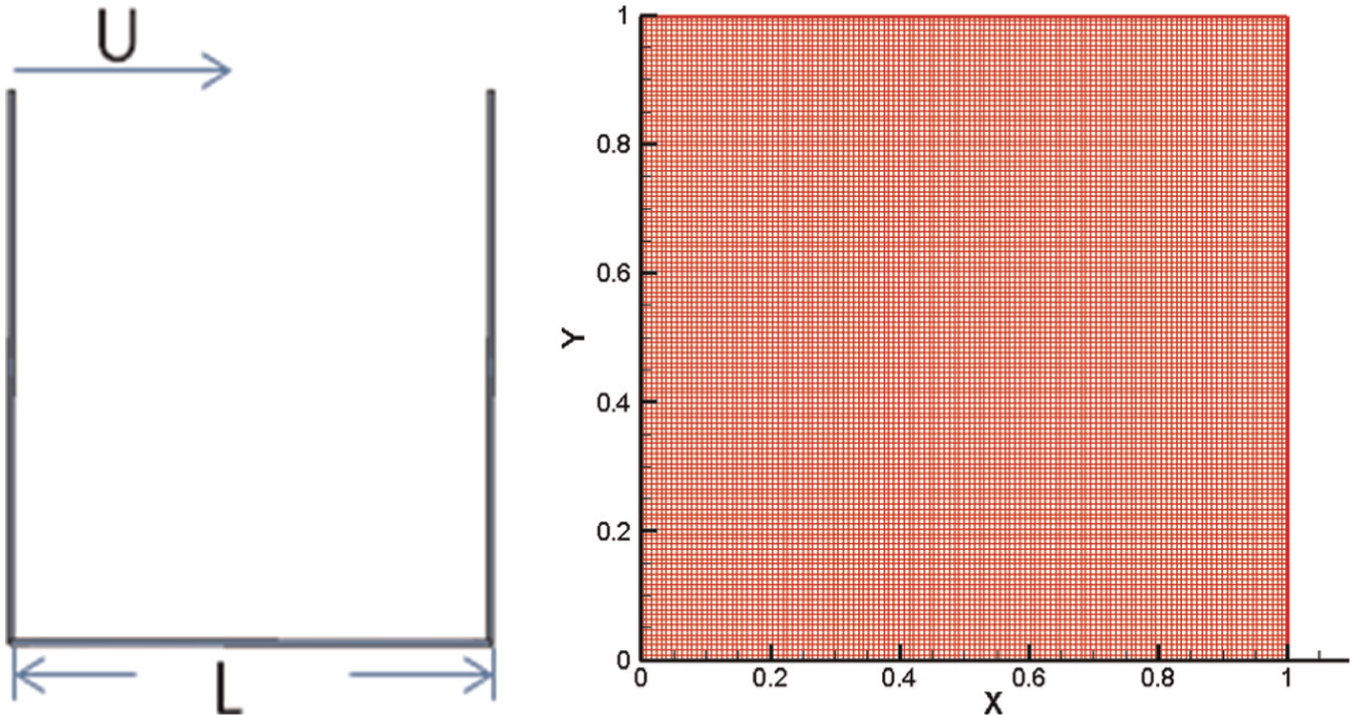
Computational domain and grids.
Figure 7 reveals the stream line and vortex contours at Reynolds number 7500 and U = 0.1. From this figure, the complex vortex structures are found, main vortex lies in the center of the cavity, small vortex also exists in the corner of the cavity around the main vortex, and a second vortex is also clearly seen in the lower right of the cavity. Detailed quantitative comparisons of the vortex position can be found in Table 2 in order to show the ability of the present LBM/LES for simulating high Reynolds flow. Compared with Ghia et al.’s 15 results, the calculated results in the article can keep consistent with them for the different vortex positions. It is expected that LBM/LES is used to simulate high Reynolds number flow around the complex bodies.

Stream lines and vortex contours for cavity flow.
Comparisons of vorticity positions inside the cavity.

NACA0012 airfoil at high Reynolds numbers
NACA0012 airfoil at high Reynolds flow is simulated at

Computational domain, boundary, and grid.
Table 3 shows the comparison of lift and drag coefficients between the present and the referred results for
Detailed comparisons of Cl
and Cd
at

B-L model: Baldwin-Lomax model; LBM: lattice Boltzmann method; LES: large eddy simulation; S-A model: Spalart-Allmaras model.
Detailed quantitative comparisons are performed to compare with the experimental results at
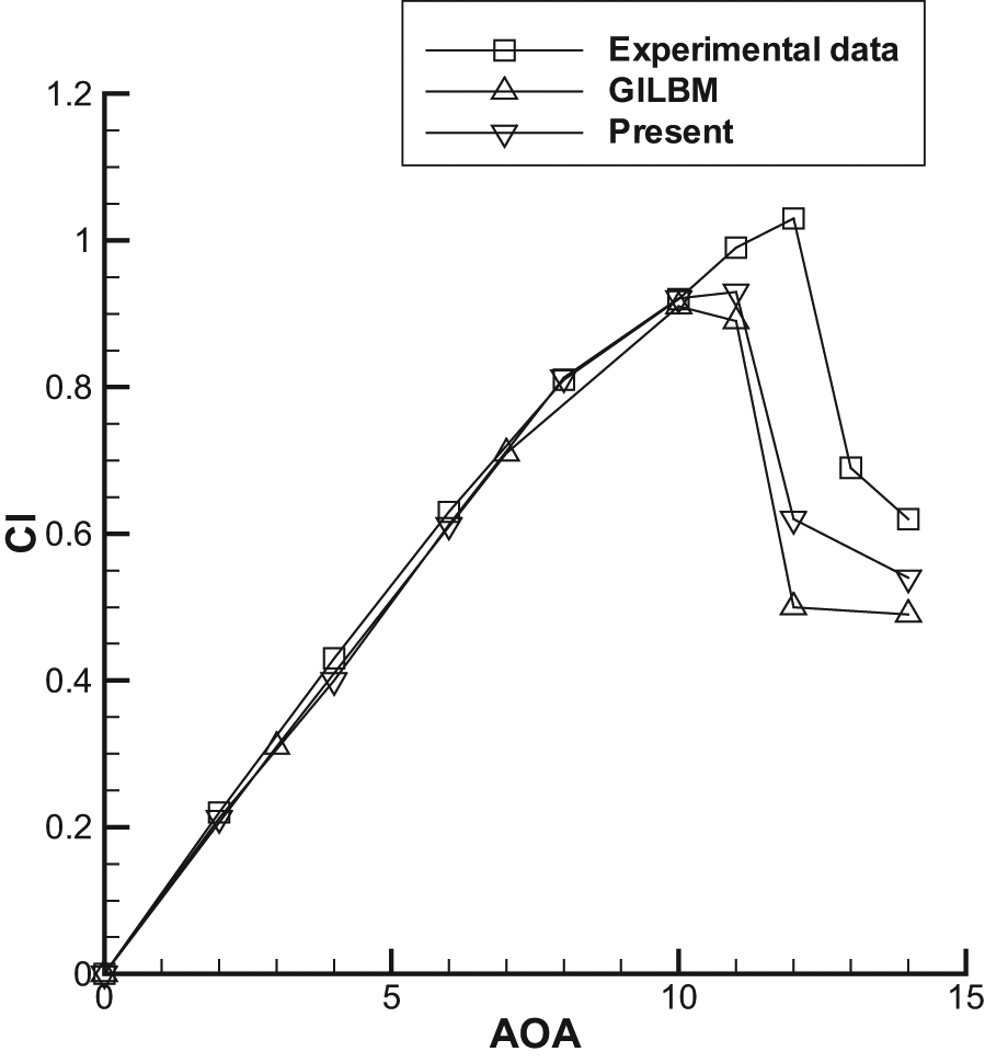
Lift coefficient versus different AOA at

Drag coefficient versus different AOA at
Conclusion
Compared with the other methods, the present method combining the LBM and LES model could solve the problem at high Reynolds numbers’ flows. As one of all subgrid models, Smagorinsky model can provide a positive eddy viscosity to represent small-scale energy damping. For the treatment of boundary condition, non-equilibrium bounce-back scheme has been applied on the far-field boundary in the computational domain. The boundary condition for the particle distribution functions on the curved wall is handled using second-order accuracy scheme. Lift and drag evaluation in the LBE takes momentum-exchange method for curved boundary. The developed program is first to simulate low Reynolds number circular cylinder flow field; it proves that it could provide a possibility to model high Reynolds problems using the present method. Next, lid-driven cavity flow and NACA0012 airfoil flow are calculated to show the ability of combining LBM with LES for simulating high Reynolds number flow. Some comparisons demonstrate that the present calculated results could obtain good agreement with the experimental ones.
Footnotes
Academic Editor: Oronzio Manca
Declaration of conflicting interests
The authors declare that there is no conflict of interests.
Funding
This work was supported by Special Foundation of China Postdoctoral Science (grant no. 201104565), National Natural Science Foundation of China (grant no. 11272151), and the Fundamental Research Funds for the Central Universities (grant no. NS2015063).