
Abstract
Dissipative particle dynamics is a particle-based mesoscopic simulation method. Classic dissipative particle dynamics cannot be used to simulate heat transfer in fluids since the total energy of the system is not conserved. In this article, two-dimensional unsteady heat conduction is first investigated using dissipative particle dynamics with energy conservation. The energy conservative dissipative particle dynamics results are compared with the FLUENT simulation data, and it demonstrates that they are in good agreement with each other. Then, forced convection heat transfers in microchannel of the same wall temperature and different wall temperatures are simulated, respectively, by using periodic boundary condition of dimensionless temperature. The results show that the velocity, temperature, and dimensionless temperature distributions are consistent with theoretical results. Finally, we give a qualitative analysis about the applicability of the energy conservative dissipative particle dynamics approach in simulating flow and heat transfer in rough microchannel.
Introduction
In recent years, with the rapid development of microelectro mechanical systems (MEMS), the demand for probing the mechanism of the microscale flow and heat transfer problems is increased, in which the Knudsen number is probably larger or equal to unity. This restricts the applicability of continuum mechanics in these types of problems. The most straightforward and accurate approach is probably the molecular dynamics (MD). Sofos et al. 1 studied how wall properties control diffusion in grooved nanochannel by using MD method and achieved some valuable conclusions. However, MD is too inefficient for mesoscale simulations due to the vast computing resources required. 2 A number of “coarse-grained” approaches have been suggested and developed to simplify the underlying microscopic model while retaining the essential physics. Although Brownian dynamics simulations (BDS), lattice gas automata (LGA), and lattice Boltzmann method (LBM) are mesoscale simulation methods, it is difficult for BDS to deal with a complex flow field and for LGA and LBM to cope with complex fluids. 3 Dissipative particle dynamics (DPD) has emerged as a promising new mesoscale simulation technique introduced by Hoogerbrugge and Koelman. 4 It is a coarse-grained, particle-based simulation method. 5 In the DPD system, the basic unit is a set of discrete momentum carriers called particles, moving in continuous space and in discrete time steps. The momentum carrier is a coarse-grained entity of mass m in a three-dimensional simulation domain. The particle’s motion represents the collective dynamic behavior of a large number of molecules (a fluid “particle”). 6 DPD conserves not only the number of particles but also the total momentum of the system and satisfies Galilean invariance and the detailed balance equations. Since its introduction, DPD has been widely used for simulations of various complex fluids and complex flows, such as porous flow, 3 colloidal suspensions,7–9 polymer suspensions, 10 or multicomponent flows. 11
However, classic DPD can only be applied to simulate isothermal systems, and modeling of thermal systems was not possible since the total energy of the classic DPD system is not conserved. 12 In order to solve this energy conservation drawback, Español 12 and Avalos and Mackie 13 introduced an internal energy variable and a temperature for each particle in the DPD system, which enabled the modeling of heat transfer. This DPD model with energy conservation is called energy conservative dissipative particle dynamics (eDPD). Each particle in eDPD system is associated with its internal energy in addition to other quantities such as mass, position, and momentum.
The eDPD has been used to model a few of heat transfer problems. By using eDPD, Ripoll et al. 14 studied the model of eDPD for the simple case of thermal conduction, and it is shown that the model displays correct equilibrium fluctuations and reproduces Fourier law. Chaudhri and Lukes 15 presented a multicomponent framework of the eDPD; the framework was validated for the special case of identical components in one and two dimensions. Abu-Nada 16 used eDPD to investigate conduction heat transfer in two dimensions under steady-state condition. Various types of boundary conditions were implemented to the conduction domain. It was found that DPD appropriately predicts the temperature distribution in the conduction regime. Abu-Nada 17 also used eDPD to study natural convection via Rayleigh–Benard problem and a differentially heated enclosure problem. The eDPD results were compared with the finite volume solutions, and it was found that the eDPD method predicts the temperature and flow fields throughout the natural convection domains properly. The eDPD model recovered the basic features of natural convection. Abu-Nada 18 further studied natural convection in liquid domain over a wide range of Rayleigh numbers. By using eDPD, Yamada et al. 19 simulated forced convection in parallel-plate channels with boundary conditions of constant wall temperature and constant wall heat flux. The periodic boundary condition of the dimensionless temperature in the flow direction was adopted. The results agreed well with the exact solutions to within 2.3%. Yamada et al. 20 also applied eDPD to heat conduction in nanocomposite. The effects of the interfacial thermal resistance and the Brownian motion of nanoparticles were incorporated in the model. The results agreed well with the experimental results. Qiao and He21,22 simulated heat conduction in nanocomposite materials and nanofluids by using eDPD. Their simulation results indicate that the eDPD method can be a versatile method for studying thermal transport in heterogeneous materials and complex systems. More recently, Cao et al. 23 used eDPD to simulate natural convection in eccentric annulus. A numerical strategy is presented for dealing with irregular geometries in DPD system. And it was found that the temperature and flow fields for the natural convection in complex geometries are correctly predicted using eDPD. Cao et al. 24 also adopted eDPD to simulate the mixed convection in eccentric annulus. The results show that the forced, natural, and mixed convection flow and heat transfer in complex geometries are correctly predicted using eDPD. Furthermore, Li et al. 25 verified the eDPD model for reproducing correctly the temperature-dependent properties including Schmidt number and Prandtl number and analyzed the relationships between the dynamic properties of eDPD fluid and the parameters in the dissipative and random forces. Moreover, Willemsen et al. 26 used the eDPD method to model phase change with the consideration of energy equation.
In the classic DPD method, particles may penetrate the wall because of the soft potentials used. Several methods have been proposed for the wall boundary condition to reintroduce these particles back. In general, there exist two main approaches. In the first approach, the fluid–wall interactions are represented by certain effective forces with the combination of proper reflections to prevent particle penetration. 27 The second and the most widely used approach is based on the representation between the fluid and the wall particles that combine freezing particles along the walls of the physical domain with different wall reflection laws, for example, simple fluid, 28 colloidal suspension, 8 and a polymer solution between bounded walls. 29 No matter which methods they take, the aim is to achieve the no-slip boundary condition. In this work, we implement the no-slip boundary condition to the fluid flow in microchannel.
Although quite a number of investigations have been carried out to study the heat transfer problems by using eDPD, it is still necessary to further examine the potential of the eDPD method. In this study, the eDPD was used to simulate fluid flow and forced convective heat transfer in microchannel. The article is organized as follows. In section “Numerical method,” we give a brief review of eDPD schemes. In section “Results and discussion,” we present the validation of the eDPD model by the simulation of two-dimensional (2D) heat conduction. Numerical results for forced convection in microchannel channels are also presented. We conclude with a brief summary in section “Conclusion.”
Numerical method
eDPD
Similar to the classic DPD method, each eDPD particle is still considered as a coarse-grained particle, which represents a cluster of actual fluid molecules instead of atom/molecule directly.
25
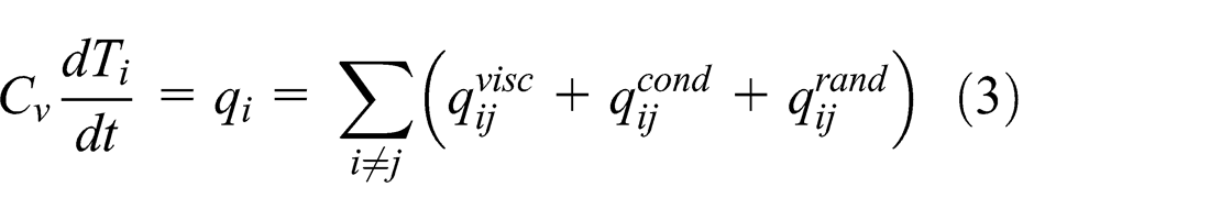
The time-evolution of eDPD particles is governed by conservation of momentum and energy. For a simple eDPD particle
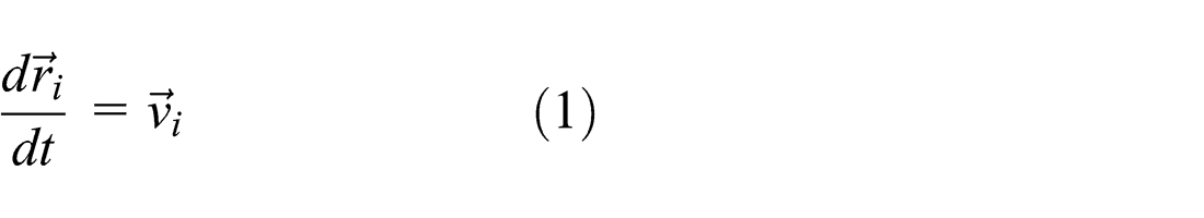

where


The energy equation (3) includes three parts, in which viscous heat flux


where
All of the weight functions decrease monotonically with the increase in the particle–particle separation distance and vanish for

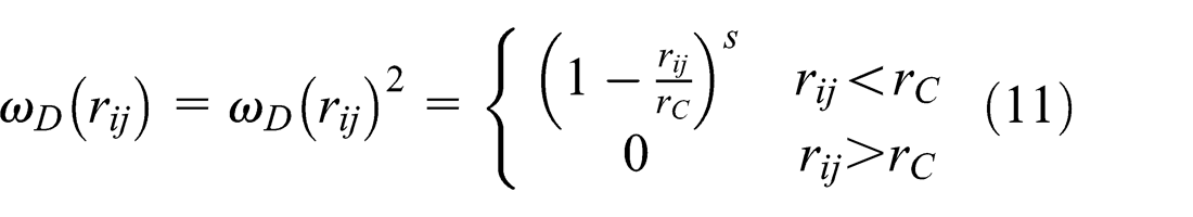
In order to improve the viscosity of the fluid,
The weight functions

where


where

where
Initial and boundary conditions
The simple eDPD particles are initially generated at the face-centered cubic (FCC) lattice cites, and it is expected that the density of the fluid is 4. The initial velocities of the fluid particles are set randomly according to the given temperature, but the wall particles are frozen.
For the nanoscales, since the continuum assumption is not satisfied in confined problems, the no-slip boundary condition is not valid. 31 In this work, we used eDPD to model the flow and heat transfer in mesoscale; similar to a few of cases, 32 the no-slip boundary condition for the velocity was imposed. As shown in Figure 1, in order to implement no-slip boundary condition and prevent particles from penetrating the walls, the solid walls are represented by using three layers of frozen particles according to Fan et al., 32 in which a thin layer near the wall is assumed, and particles in this layer always leave the wall. Additionally, we enforce a random velocity distribution in this layer with zero mean corresponding to a given temperature.

Sketch of boundary condition.
In order to mimic an infinite system, periodic flow boundary conditions are applied on the fluid boundary of the computational domain in the x and y directions. However, for the periodic thermally developed region, the dimensionless temperature field repeats itself periodically. The formula of dimensionless temperature for the case of constant wall temperature boundary condition is shown below 19
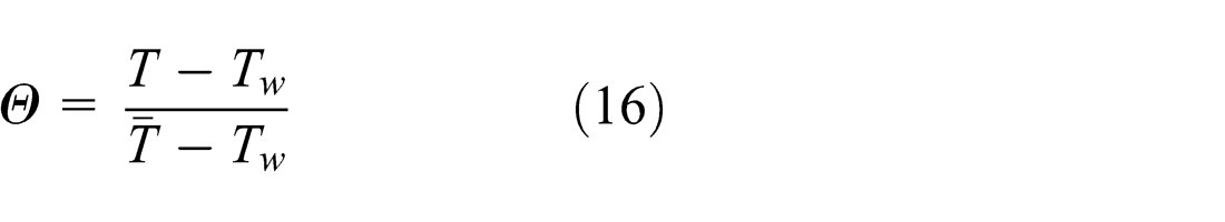
where

where the average temperature

For the periodic thermally developed region, the dimensionless temperature satisfies the following relationship
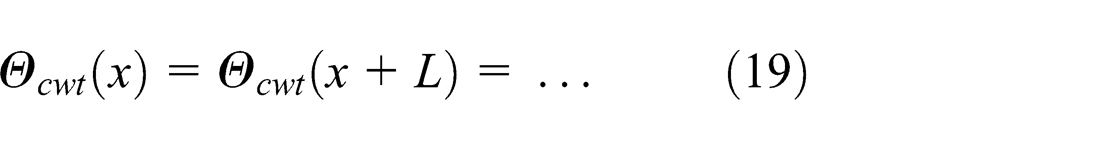
When a particle moves out of the simulating domain at one side, the average temperature of this side cross section can be calculated by equation (18). Substituting the average temperature into equation (16), the dimensionless temperature
Results and discussion
Validation of the methodology
Similar to Abu-Nada,
16
in this study, the eDPD model is validated by simulating a 2D heat conduction problem, and the results are compared with the FLUENT simulation results. Here, we simulated the 2D unsteady heat conduction, while in Abu-Nada,
16
the steady heat conduction was studied. The schematic of the solution domain and the corresponding boundary conditions of this problem are shown in Figure 2. Three sides of the rectangular plate are maintained at a constant high temperature

Schematic of the computational domain for 2D plate conduction.

(a) Time-evolution of the temperature profile at the mid-slab height (y = 0) and (b) time-evolution of the temperature profile at the mid-slab width (x = 0) (solid lines: FLUENT; symbols: eDPD).

Steady-state temperature isotherms (solid lines: FLUENT; dashed lines: eDPD).
Forced convection heat transfer in microchannel with smooth surfaces
For the simulation of forced convection heat transfer in microchannel, the simulation parameters used are given in Table 1. Note that
Simulation parameters.

Case I: same wall temperature
In this case, the temperatures at top and bottom walls are kept the same, that is,

Schematic of the solution domain.

Time-evolution of the temperature profile.
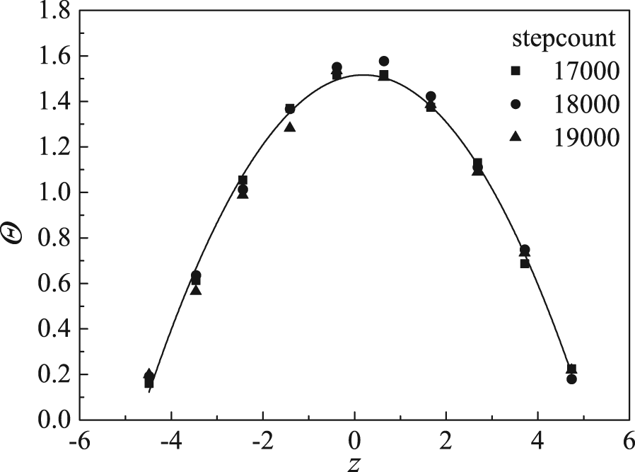
Dimensionless temperature profile.
Sofos et al. 33 examined the effect of channel width and system temperature on diffusion coefficient, shear viscosity, and thermal conductivity in the MD simulations. They mentioned that the rise in temperature results in a significant decrease in viscosity. Therefore, the effect of viscosity and its variation cannot be ignored and is also considered in this work.
The kinematic viscosity of the eDPD fluid can be computed by 34
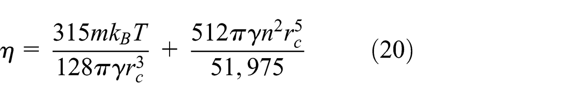
Using the above-mentioned parameters (i.e. m = 1,rc = 1, n = 4, T = 1.0, and γ = 4.5), the value of the kinematic viscosity of the eDPD fluid is 2.402. Furthermore, for the Poiseuille flow, the velocity distribution in the x direction across the channel can be calculated 18 by
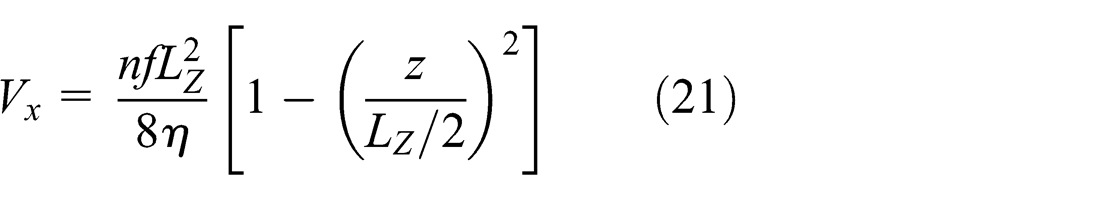
And the maximal velocity of
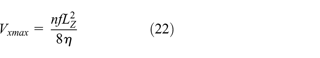
As shown in Figure 8, the simulated maximal velocity for this case was 0.341, and the difference from the analytical solution calculated by equation (22) was 18%. The difference is larger, and it is mainly due to the variation in the viscosity with the variation in the temperature. In fact, in this case, the fluid temperature approaches the wall temperature infinitely for enough time steps. So, the wall temperature could be adopted as the approximations of the fully developed fluid temperature to calculate the maximal velocity by equation (22). The newly calculated value of the analytical solution is 0.345, and the difference from the simulated value of 0.341 is only about 1.2%. Figure 8 shows the comparison between the eDPD and the analytical solutions, and it is found that they are in good agreement with each other.

Velocity profile.
The Nusselt number (Nu) is the ratio of convective to conductive heat transfer, and it is given by the following equation

where

where the temperature gradient is given by

So, the convective heat transfer coefficient of the fluid is expressed as

Substituting equation (26) into equation (23), the Nusselt number (Nu) is expressed as

Three layers of fluid particles close to the wall are chosen to calculate the Nusselt number. So, the variation of density near the wall has a great effect on the final results. As shown in Figure 9, particle distribution is relatively uniform when adopting the bounceback boundary condition mentioned in section “Initial and boundary conditions” in which

Density profile.
Different wall temperatures
The forced convection in which the temperatures at top and bottom walls are different was also simulated. The schematic of the computational domain is shown in Figure 10. A body force

Schematics of the solution domain.

Time-evolution of the temperature profile.

Velocity profile of forced laminar convective heat transfer.
As shown in Figure 13(a), density distribution is horizontal as similar to that simulated by the classic DPD method. However, the character of fluids such as water is that density distribution depends on the temperature distribution, that is, lower density for the hot fluid and higher density for the cold fluid. Then, we follow the method used by Li et al.
25
to regulate the conservative coefficient

Density profile. (a) a ijf = 18.7 and (b) a ijf = 18.75kB (Ti +Tj )/2.
Forced convection heat transfer in grooved microchannel
In this section, the problem of forced convection heat transfer on rough surface is studied using the eDPD approach and compared with FLUENT solution. The fluid in this microchannel is incompressible, Newtonian fluid, as shown in Figure 14. The temperatures of the hot and cold walls are maintained at a constant 1.0 and 1.5, respectively. The initial temperature of the eDPD fluid particles is set at 1.0. Other parameters are the same as before. Introducing the eDPD parameters into the predictions, equation (20) gives

Schematic of the solution domain.
Comparison between present eDPD simulation and FLUENT solution for the temperature isotherm is shown in Figure 15(a) and (b). Figure 16 shows the streamline of flow around the single obstacle in the channel. There is a clockwise vortex near the front of the lower left corner, and a clockwise recirculation is also developed downstream from the obstacle. It is found that the eDPD simulated results are in agreement with FLUENT data. These results demonstrate that the eDPD is effective in simulating this kind of flow and heat transfer. However, the size of the vortexes between the eDPD and FLUENT results is slightly different. We guess it may be caused by the boundary condition mentioned in section “Initial and boundary conditions,” and we expect it will be our future work.

Temperature isotherms of flow around the single obstacle in the channel (a) FLUENT and (b) eDPD.

Streamline of flow around the single obstacle in the channel (a) FLUENT and (b) eDPD.
Conclusion
In this article, forced convection heat transfer problems in microchannel were simulated numerically by eDPD. This concludes as follows.
The 2D unsteady heat conduction problem was simulated by eDPD. The results agree well with FLUENT results.
For the simulation of the forced convection on smooth surface that the temperatures of the upper wall and lower wall are different, the distribution of temperature is linear, which is in a good agreement with the theoretical solution. Since the viscosity changes with the temperature, the velocity distribution is asymmetric. The peak of the velocity profile shifts to the side corresponding to the high temperature fluid. In the situation that the upper wall and lower wall temperatures are same, in order to calculate the viscosity correctly, the variation in the fluid temperature should be taken into account. Furthermore, the simulated maximum velocity agrees well with the analytical value.
Finally, we give a qualitative analysis about the applicability of the eDPD approach in simulating flow and heat transfer in rough microchannel, and a good agreement is observed with each other. Above all, the eDPD model is a powerful tool in simulate flow and heat transfer problems. In the future work, we will extend the application of eDPD to simulate flow and heat transfer in more complex structures.
Footnotes
Acknowledgements
The grants are gratefully acknowledged.
Academic Editor: Pietro Scandura
Declaration of conflicting interests
The authors declare that there is no conflict of interest.
Funding
This work was supported by the National Natural Science Foundation of China (Grant Nos 51276130 and 10872152) and the Fundamental Scientific Research Foundation for the Central Universities of China (Grant No. 125065).