A methodology for semiautomatic generation of finite element models: Application to mechanical devices

Abstract

In this work, a methodology to create parameterized finite element models is presented, particularly focusing on the development of suitable algorithms in order to generate models and meshes with high computational efficiency. The methodology is applied to the modeling of two common mechanical devices: an optical linear encoder and a gear transmission. This practical application constitutes a tough test to the methodology proposed, given the complexity and the large number of components that set up this high-precision measurement device and the singularity of the internal gears. The geometrical and mechanical particularities of the components lead to multidimensional modeling, seeking to ensure proper interaction between the different types of finite elements. Besides, modeling criteria to create components such as compression and torsion springs, sheet springs, bearings, or adhesive joints are also presented in the article. The last part of the work aims to validate the simulation results obtained with the methodology proposed with those derived from experimental tests through white noise base-driven vibration and hammer impact excitation modal analysis.

Introduction

The current trends in finite element method (FEM) software commercial packages are based on associative modules between the models that contain the geometrical information (computer-aided design (CAD) model) and the model over which the simulation tasks are developed (computer-aided engineering (CAE) model). Basically, this means that the software module corresponding to the finite element model is able to recognize the parameters that have been interactively defined while building the geometrical model and to adapt the CAE model to the changes introduced on these parameters. Unless in very particular cases, the model obtained by this procedure usually needs a certain treatment before beginning the simulation stage. The direct use of the models produced by this way is invalidated because of the fact that CAE and CAD are significantly different disciplines to require dissimilar model representations. ¹ From this point of view, there are a large number of works that try to automate the process of adaptation of the CAD model to the simulation environment.^2,3 Most of the works deal with feature suppression or detail removal,^4–6 and others focus on the automation process in order to obtain ready-to-mesh models from highly coupled variable topology multibody problems.^7,8 In the field of automatic generation of finite element models, in Shephard ⁹ is asserted that the transition to the automated techniques may not be smooth, one of the reasons being that the finite element analyst could feel uncomfortable not being able to manipulate the model and define information on the individual node and element level. However, other variables such as mesh parameters will still be on user’s part. This statement agrees with the methodology followed in this work. Particularly referring to the methodology proposed, an algorithm for automatic structured mesh generation can be found in the literature, ¹⁰ focusing on the sequence of elements’ and nodes’ numbering in order to create the mesh. A similar procedure is described in this work but referred to the areas’ generation of the geometry model instead of direct elements’ generation since the solid modeling technique has been used.

In this work, a methodology to develop finite element models based on the parametric language APDL is presented. The methodology proposed, even though it is not an automated process in the sense that the programmer must determine the parametric relations between the design variables, could be considered as a semiautomatic way of creating finite element models, since the guidelines to be followed in order to get a systematic implementation of finite element models are provided. The guidelines are based on the current trends of automatic generation of finite element models such as geometrical idealization, feature and detail removal, cell fragmentation, dimensional reduction, and associativity maintenance. Although the methodology can be applied to any device, it is presented through the modeling process of two common mechanical devices: an optical linear encoder and a gear transmission to perform dynamic analysis.

Methodology modeling strategy

For the sake of clarity, the methodology proposed is presented here step by step in order to facilitate its implementation.

Classification of components

The first step consists of distinguishing between the so-called volumetric and joining components. In order to accomplish this stage, study the possibility of applying dimensional reduction to the different components and also study the coupling between components.

In the present methodology, it is proposed to create first the volumetric components by means of solid modeling and afterward to create the so-called joining components by means of direct generation, that is, inserting the finite elements that form these components between the nodes of the generated volumetric components’ mesh. The main reason for this, is that, in case the solid modeling technique would also be used for the joining components, an exhaustive fragmentation of the geometrical entities that constitute the final model would be required, in order to connect all the components’ meshes properly. This approach would result in an unnecessary increase in the complexity of the model.

Establish the sequence of modeling

One thing to be added to what has been stated and that has a relative importance in the sequencing of the components to be modeled is the choice of the first component. It has to be taken into account that the geometrical variables of the different components are interrelated between them in such a way that those parameters defined for the first component would be transferred to the rest of the device’s components. Apart from this, as the modeling process goes on, the level of difficulty reduces because of a more restrained model.

The first question that arises when beginning the modeling process is to determine the sequence of the components to be modeled. In order to do this, the main components can be identified as those which have implicitly defined in their geometry the variables that better describe the system as a whole.

The key step in doing so is the choice of the first component. Identify the dimensions that characterize the device and choose as the first component the one that has the highest number of dimensions the other components can be referred to. Also, look for the component that in some way “encircles” the other components.

Features’ and details’ suppression

The next step in the methodology proposed consists of features’ and details’ exclusion. Very often, the mechanical design of a particular component presents a high number of details that, although they are created with a specific functionality like coupling to other components, can have a negligible influence on the behavior of the component depending on the analysis to be done. Modeling these details entails a considerable increase in computational cost in several senses. On one side, there is an increase in complexity in the modeling procedures impeding systematic sequences of commands of the so-called bottom-up, having to resort sometimes to Boolean operations with a higher computational cost. On the other side, irregular geometries increase the difficulty and sometimes prevent from structured meshes. In a structured mesh, it is easier to control the size and shape of the finite elements, allowing mesh variations over certain regions without having to increase indiscriminately the number of elements in order to fulfill elements’ shape factors.

For volumetric components, frequently this step is reduced to use the volume region that encloses the component. For joining components, look for simplified models derived from the dimensional reduction applied in the first step.

Cell fragmentation

This step consists of the tessellation of the cross-sectional areas of the volumetric components. Basically, divide the areas of the exterior components into rectangles and prolong divisions into interior components. Another aspect and no less important of structured meshes is that it facilitates the compatibility between geometrical and mesh parameters, what allows associativity maintenance all through the modeling process. For instance, it has to be taken into account that joining components need confronted structured meshes in order to assure a proper lining up and also need an appropriate spatial discretization to their positioning, since their creation is by means of direct generation. Within this context, another key concept of the introduction references takes part in the methodology proposed: cell fragmentation. The fragmentation of the geometry in rectangular entities is needed in order to assure the same number of elements in confronted lines to generate the structured mesh. There are several ways to accomplish the tessellation process, but it can be systematized in three steps. The first one would be to divide each one of the areas that make up the cross section of the exterior components in rectangles. In the second step, it is needed to lengthen each one of the divisions made in the previous step toward the interior components. The third and final step consists of increasing the tessellation level depending on the joining components. Normally, the fulfillment of the first two steps can be carried out without unforeseen difficulties. The final step requires a higher effort.

Volumetric components’ modeling

Once the model has been determined according to the strategy explained in the previous sections, the generation of volumetric components is systematic. The procedure consists of a bottom-up process. First of all, the geometrical coordinates of the points that will be the base for the construction of lines, areas, and volumes have to be defined. It has to be taken into account that the parametric relations between the different geometrical variables are established when defining these point’s coordinates. The point’s definition allows controlling the numbering that the software assigns in order to identify them. This fact constitutes a great advantage over an up–bottom modeling, in which it is not possible to have control over numbering and hence, the modeling process cannot be easily systematized. The second stage consists of introducing the lines between the points defining at the same time the number of finite elements that will be placed over the lines. This is a key step in the sense that confronted lines have to share the same number of divisions in order to achieve a structured mesh, and, also, the relations between these divisions with the geometrical parameters previously defined in the introduction of points have to be taken into account. The determining of the number of divisions is influenced by several factors, but it should be increased considering the particular geometry of the component, the expected gradient of results, and the conditionings relative to the shape factors of the finite elements. It is advisable to include a factor controlling the mesh in a global way, apart from that referred previously as the number of divisions, since the latter only works locally. Once the points and lines have been defined, the next stage consists of the rectangular areas’ generation obtained by means of the tessellation process. In order to do this, only the geometrical points that form the area corners have to be selected and next only those lines that share two of these points have to be selected. As soon as the area is delimited only by the lines that make it up, its generation is straightforward. The final volumetric component composed of three-dimensional finite elements is obtained sweeping the two-dimensional finite elements’ mesh of the cross-sectional areas along a perpendicular line, defining previously its number of divisions in order to set the final dimension of the three-dimensional finite elements. This last stage can be systematized too, considering when generating the areas by the tessellation process that in their generation sequence each area shares only one line with the previous area until it is possible, and then continues with those sharing two lines, and so on. If this rule is followed, the process can be programmed into a sequence of as many *DO loops as many groups of areas have been done taking into account for the assortment the number of lines shared in the area’s generation.

Summarizing, first define the corner points of the rectangles obtained in the previous step introducing in their coordinates the parametric geometrical relations. Second, define the lines between the corner points assigning them the same number of divisions to opposite lines. Use a factor common to all mesh parameters to control the mesh globally. Afterward, select only the corner points of each one of the rectangles and then select the lines that belong only to these points in order to generate each one of the areas. Take into account the sequence of generation to create first those areas sharing only one line and continue with those sharing two lines, then three lines, and so on. Finally, sweep the bi-dimensional mesh along the perpendicular direction to create the final volumetric component.

Although the volumetric components’ modeling has been presented making use of quadrilateral and cubic elements, it can be easily implemented to make use of triangular and wedge elements.

Joining components’ modeling

Insert the finite elements that form the joining components between the volumetric components’ meshes by means of direct generation. Once the three-dimensional elements have been created, the next step in the methodology proposed is just to connect them by the so-called joining components. The main difference with volumetric components that have been created from a basis of geometrical entities is that it is proposed to model joining components by direct generation, which means that we have to use the nodes of the mesh created in the previous stage, inserting between them those finite elements defined for the joining components.

Establish constraint equations

Apply the compatibility relationships between the rotational degrees of freedom of the joining components and the translational degrees of freedom of volumetric components. This methodology is based on the parametric language APDL. One of the main advantages of APDL over the current trends of other finite element’s software is that it allows a high interaction with the different entities that make up the final model, geometrical as well as mesh entities. This possibility of interaction opens a wide door to a variety of alternatives to model the components being the modeling process not limited to a particular restrained procedure of the software used.

In the next sections, we shall apply this methodology to two different but very common mechanical devices: a precision positioning device, linear optical encoder, and a gear transmission.

Optical encoder’s modeling

The mechanical design of the encoder under study is presented and detailed in López et al.^11,12 Figure 1 shows a representation of the main components of its mechanical design. As it can be observed, the coupling of the scanning module and the scale is done by means of compression and torsion springs that assure a proper guidance of module’s motion along the measuring length. The scale is attached by means of an adhesive tape to one of the walls of the housing, which covers the components preventing them from possible sources of contamination.

Figure 1.

Representation of the main components in the mechanical designs of the linear encoder under study. 1: scale; 2: housing; 3: head; 4: scanning module; 5: sealing lips; 6: compression springs; 7: torsion springs; 8: roller bearings; 9: photodetectors’ board.

Classification of components and sequence of modeling

According to the described methodology, the first question that arises when beginning the modeling process is to determine the sequence of the components to be modeled. The device under study is just a position sensor, what makes the measuring length of the instrument the geometrical dimension that characterizes the encoder in the best way possible. Hereafter, we can define the main components as those featuring this geometrical dimension. In our case, we have three components that define the encoder’s measuring length: the scale, the housing, and the adhesive that joints both components.

In order to accomplish this assortment, considering the possibility of applying dimensional reduction to the different components is proposed. In this sense, there are several encoder’s components that clearly meet a modeling by means of volumetric finite elements. These components are the scale, the housing, the scanning module, and the head of the encoder. It can be observed that the role of the rest of the components such as the compression springs, the torsion springs, the adhesive bonded joint, and the bearings is just to define how the volumetric components interact between them. Besides, it can also be noted how these joining components have at least one geometrical dimension much lesser than the rest of the dimensions that define their geometry. In this sense, the choice of the housing instead of the scale has some advantages. On one side, a higher number of geometrical parameters over which the rest of the components can be referred to and, on another side, since the housing covers the rest of the components their dimensions present a restricting character to the rest of the geometrical variables, making easier the modeling process. This is what we referred to in the sequence of modeling section when it was stated to choose as the first component the one that “encircles” in some way the other components.

Features’ and details’ suppression

The next step in the methodology proposed consists of features’ and details’ exclusion. To illustrate this step, Figure 2 shows the real geometry of the housing with the scale and its geometry idealization by means of details’ suppression. As it can be observed in this figure, the first and the second modes of vibration of the housing wall are accurately reproduced by the idealized model, and both models differ in frequency values only a 0.76% for the first mode and 1.93% for the second mode.

Figure 2.

Geometry idealization: (a) first housing wall mode of vibration with a difference in frequencies between models of 0.76% and (b) second housing wall mode of vibration with a difference in frequencies between models of 1.93%.

Cell fragmentation

The next step consisting of the tessellation procedure, as it has been stated before, can be systematized in three steps. The first one would be to divide each one of the areas that make up the cross section of the exterior components (housing and head) into rectangles. In the second step, it is needed to lengthen each one of the divisions made in the previous step toward the interior components (scale and scanning modulus). The third and final step consists of increasing the tessellation level depending on the joining components (adhesive bonded joint and compression and torsion springs). Normally, the fulfillment of the first two steps can be carried out without unforeseen difficulties. The final step requires a higher effort. For example, if the adhesive is only to be applied over the base of the scale, the tessellation level reached represented in Figure 3(b) would be enough. However, if the adhesive tape is going to be applied also over the thickness, it is needed to introduce a new division in the housing (marked with a square in Figure 3(c)) to assure opposite nodes with those corresponding to the scale. Another specific example of the third step is that represented in Figure 3(d) with a circle. In order to confront nodes in the pressure points of the torsion springs, it is needed to create a division of the scanning module’s area at the midpoint of scale’s thickness. The compatibility between the mesh of the scanning module and the scale for this region can be achieved by means of a proper number of finite elements across glass thickness, without having to resort to a higher level of tessellation. Hence, the importance of the associativity maintenance between the geometrical parameters and those corresponding to the mesh all through the modeling process can be noted.

Figure 3.

Tessellation process: (a) divide areas of exterior elements into rectangles, and (b) prolong divisions into interior elements. (c and d) Take into account particularities of the joining components to increase the level of tessellation.

Volumetric components’ modeling

As it has been stated in the methodology modeling strategy section, the first thing to do is to define the corner points of the rectangles obtained in the previous step introducing in their coordinates the parametric geometrical relations. Second, define the lines between the corner points assigning them the same number of divisions to opposite lines. Use a factor common to all mesh parameters to control the mesh globally. Afterward, select only the corner points of each one of the rectangles and then select the lines that belong only to these points in order to generate each one of the areas. Take into account the sequence of generation to create first those areas sharing only one line and continue with those sharing two lines, then three lines, and so on. Finally, sweep the bi-dimensional mesh along the perpendicular direction to create the final volumetric component. Automated process to generate the three-dimensional elements is shown in Figure 4.

Figure 4.

Automated process to generate the three-dimensional elements.

Joining components’ modeling and constraint equations

Regarding the practical application of the proposed methodology, the linear optical encoder under study, compression springs have been modeled by means of one-dimensional bar finite elements with three degrees of freedom at each node defining the spring stiffness through the bar axial stiffness. Cross-sectional area value has been chosen in such a way that the finite element presents a suitable visual aspect with the whole geometry set. Since spring length is determined by the space between the head and the scanning unit, Young’s modulus is the variable to set the stiffness constant of these springs. Besides, it is needed to define another variable regarding the initial strain of these compression springs because of the fact that they are compressed at mounting, exerting pressure on the scanning module which alters its dynamic behavior. Regarding positioning of the finite element between the nodes of the preexisting mesh, the procedure can be systematized in two stages. By means of an algorithm, in the first stage the positioning parameter value is compared with each one of the intervals defined by the nodes of the three-dimensional elements’ preexisting mesh. Once the two nodes whose coordinates delimit the positioning parameter value have been identified, in the second stage the compression spring finite element is placed in the nearest node.

To model torsion springs, two one-dimensional beam finite elements have been used, with six degrees of freedom per node (three translations and three rotations). Stiffness spring has been defined from the torsional stiffness of one of these elements, working the other element that forms the arm as a rigid element. Regarding torsional spring stiffness, very low values of the so-called shear coefficients and very high values of the elasticity modulus have been defined in order to achieve rigid behavior of the spring element to axial and bending strains. For their positioning, a similar procedure of that described for compression springs has been followed, taking into account that the length of the spring finite element is a function of the longitudinal number of divisions defined for the scanning module. A very important aspect when joining these elements that have rotational degrees of freedom is the definition of constraint equations in order to assure a proper transmission of forces to the three-dimensional elements that make up the volumetric components, since the latter are only configured by translational degrees of freedom. Figure 5 shows a possible choice of the degrees of freedom in order to accomplish this task. From this figure, it can be deduced that the constraint equation for rotation X is given by $U_{CZ}-U_{BZ}-d_{BC}{\theta }_{BX}=0$ . In a similar way, equations $U_{BZ}-U_{DZ}-d_{BD}{\theta }_{BY}=0$ and $U_{DY}-U_{BY}-d_{BD}{\theta }_{BZ}=0$ constrain the rotational degrees of freedom in the Y- and Z-directions, respectively.

Figure 5.

Relations between the degrees of freedom to define constraint equations between the torsional spring beam element and the three-dimensional elements.

The bearings that allow the movement of the scanning module over the scale have been modeled by means of one-dimensional finite elements which can only be compressed and not tensioned, so the scanning module can separate from the scale, if it so happens. This is just a straightforward way to model the contact that is suitable to perform dynamic analysis with the scanning module placed at a certain position along the measuring length of the encoder.

The procedure to model the adhesive bonded joint is that proposed in Loss and Keyward ¹³ and is characterized by the presence of two coincident nodes at the middle of the adhesive thickness, which are joined to the nodes of the elements that form the substrates by means of rigid elements. The main reason for this choice has to do with computational cost. It has to be considered that the thickness of the adhesive tape can be much smaller than the thicknesses of the components that it connects. Therefore, not only a very high number of three-dimensional elements would be needed to model the joint properly but also in the adjacent regions in order to fulfill conditionings relative to the finite elements’ shape factors. It is needed to insert shear and peel springs between the coincident nodes with stiffness values depending on the mechanical properties of the adhesive. Figure 6(a) shows schematically the node configuration and the elements defined. The parameterization of their positioning is the most complicated among all other joining components, since it is necessary to distinguish between interior, edge, and corner finite elements, taking into account also if the mesh varies over the surface where the adhesive is applied.

Figure 6.

Modeling of the adhesive bonded joint. (a) Schematic configuration of the elements defined, (b) representation of geometrical and mesh parameters, and algorithms for grid (c) and elements generation (d).

Optical encoder’s FEM validation

Experimental setup

The experimental technique implemented to validate the methodology proposed has its basis in the modal characterization procedures through base-driven tests carried out in Steenackers et al. ¹⁴ and Ozdoganlar et al. ¹⁵ The encoder has been subjected to white noise random vibration by means of an electrodynamic shaker, measuring vibration levels at the points of interest with a laser Doppler vibrometer. The reference to construct the frequency response functions is given by the force signal of an impedance head placed on the fixture surface next to the encoder, in order to assure the desired vibration at the base of the device under test. The acceleration signal of the impedance head has been used as the excitation system feedback. Although the laser vibrometer can take only one measurement at once, the random character of the excitation signal allows taking measurements successively over the points of interest in order to obtain the modal shapes of each one of the components of the encoder. Figure 7 shows the experimental setup and its schematic representation for the sake of clarity.

Figure 7.

(a) Photograph of the experimental setup and (b) schematic representation of the experimental setup.

Results

Figure 8 shows the first two modes of vibration of the housing wall and Figure 9 shows the first four modes of the scanning module, obtained by means of simulation (shown at right) and compared with those results obtained by the experimental tests (shown at left). Regarding the experimental vibrational shape, a cubic interpolation surface has been fit to the measurement points. Concerning housing wall vibration, the asymmetry obtained in the deformed shape of the modes is worth mentioning. Under manufacturing and mounting ideal conditions, these modes should exhibit symmetry, as it is represented in Figure 2. However, it is of interest to analyze the asymmetry obtained in the sense that it helps us to understand how the encoder is influenced by a defective manufacturing or faulty mounting conditions. One of the reasons can be due to the mounting procedure. The housing wall is supported by rubber elements that can exert more or less pressure depending on the torque applied to the fixing bolts. Another explanation can be a lack of parallelism of the housing wall which would cause a different pressure exerted by the sealing rubber on both sides of the encoder. In order to reproduce these experimental results have been necessary to include spring elements in the supports of the housing wall defining dissimilar stiffness values to both sides. In Figure 9, it can be observed how the finite element model obtained by the methodology proposed reproduces faithfully the first vibrational mode of the scanning module. Concerning the second mode, if we focus the attention to the lower area next to the head, the experimental and simulation results are very similar: there is an alternating movement between these corners of the scanning unit while the part of the scanning unit next to the upper area remains almost motionless. It has to be taken into account that the laser measures movements in the direction where it is pointing. This can be one of the reasons why the alternating movement of the lower corners that is happening in the laser direction is better registered (quantitatively speaking) than the upper area which has not a predominant movement in that direction. This would agree with the results obtained for the first mode, as the movements of this mode happen along the laser direction. These explanations also applied to the results obtained for the third and fourth modes: they are predominantly pitch modes that have no significant displacements in the direction the laser is pointing. Despite this, the simulation reproduces well again the vibration movement predominant in the measuring direction.

Figure 8.

First and second modes of vibration of the housing wall obtained by simulation (shown at right of each figure) and experimental tests (shown at left of each figure).

Figure 9.

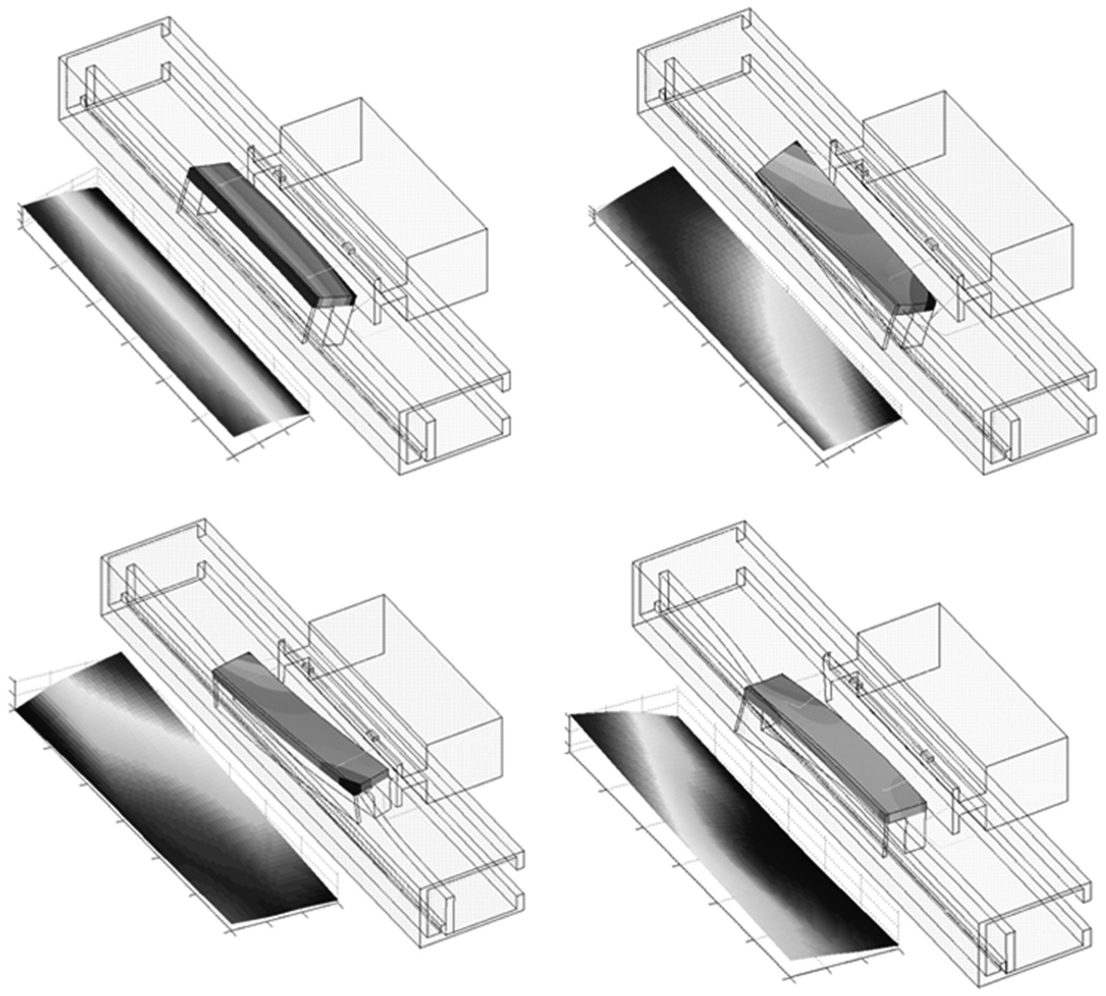
First four modes of vibration of the scanning module obtained by simulation (shown at right of each figure) and experimental tests (shown at left of each figure).

Gear transmission modeling

This section deals with the finite element modeling of a rotational component in order to demonstrate the general character of the methodology proposed and also to increase the amount of experimental data which confirms its validity. The rotational component is just an internal gear.

The modeling process in this case is quite straightforward in the sense that we are dealing only with one component. Because of this, steps regarding classification of components, sequence of modeling, joining components’ modeling, and constraint equations can be disregarded. Figure 10 shows the schematic view of the modeling process of the half tooth of the gear. From the initial geometry, the first step done is feature and details’ suppression. The geometry idealization in this case consists of lengthening the involute profile of the tooth from the addendum to the dedendum, ignoring the trocoid part of the profile. Taking into account that the analysis to be done is a modal analysis of the whole component with interest in the first modes of vibration, this detail has little influence since it is related to the vibrational modes of the tooth, which would appear at much higher frequencies. To generate the involute curve, the APDL sequence of commands given in Li et al. ¹⁶ has been used. Once these keypoints have been defined over the tooth’s profile, the rest of the points have been positioned in order to create the rectangles defined by the cell fragmentation stage.

Figure 10.

Schematic view of the modeling process of the half tooth of the gear.

The procedure to generate the three-dimensional elements is just that described in the volumetric components’ stage. In Figure 10, it can be appreciated how, once the keypoints have been introduced, all of them are joined by lines defining the rectangles, the number of elements per line, and the mesh global factor in a row. The command’s sequence to follow in order to generate the areas can be noted in the next step, which consists of selecting only those corner keypoints of the area, then only the lines that connecting these keypoints, and the last command corresponds just to the creation of the area. The next image of the figure consists of area’s meshing. In order to accomplish this step, the assignment of attributes such as material properties, real constants, and type of finite element to the areas is needed. Once the areas have been meshed, the procedure follows with the extrusion of the bi-dimensional elements. The next image consists of the creation of the perpendicular line to the areas just to sweep the bi-dimensional elements and finally obtain the three-dimensional elements represented in the last image of the figure.

The rest of the modeling process has to do with the generation of the plate that joins the gear ring to the shaft. The same procedure has been followed, but in this case, the areas have been swept along a circle’s arc in a rotational way. What we obtain in this case is a circle’s arc portion of the whole model. In order to create the component, application of symmetry is needed followed by a circular pattern generation. Some views of the complete component are shown in Figure 11 with a refined mesh. Particularly, Figure 11(a) shows a front view of the component while Figure 11(b) shows the view backward, and Figure 11(c) is a detailed view of the model of the gear where the teeth details can be appreciated.

Figure 11.

(a) Front, (b) back, and (c) detailed views of the finite element model of the internal gear.

Gear transmission FEM validation

Experimental setup

On the other side, experimental modal analysis by impact hammer has been the technique carried out in order to validate the results related to the gear model. In this case, an accelerometer has been placed at the back edge of the plate and successive impact excitations have been produced with the hammer, around the circle’s plate edge and at the middle of the plate.

Results

In order to obtain the experimental modal shapes in case of the gear, the same surface interpolation procedure has been followed. Figure 12 shows three of the modes of vibration of the gear, the experimental results being shown at left and the simulation results shown at right. The modes have been selected taking into account that those that have a predominant movement in the accelerometer measuring direction would be better represented. The first one is a motion happening along the axis of the shaft where the plate deforms forward and backward, the ring zone of the teeth moving almost like a solid rigid. This mode is very well captured by the experimental data as it can be observed in the first pair of images of Figure 12. In fact, it can be appreciated in this figure that the simulation and experimental results match quite well for all the modes considered, as their motion happens primarily in the measuring direction. In the second mode, there appear four nodal lines that allow the motion of four sectors of the plate being opposite sector’s pairs in phase. The third mode is very similar to the second mode but with more nodal lines. In this case, there appear six nodal lines dividing the motion of the plate into six sectors being the motion in phase for pairs of three sectors at angles of $2\pi /3\mathrm{rad}$ .

Figure 12.

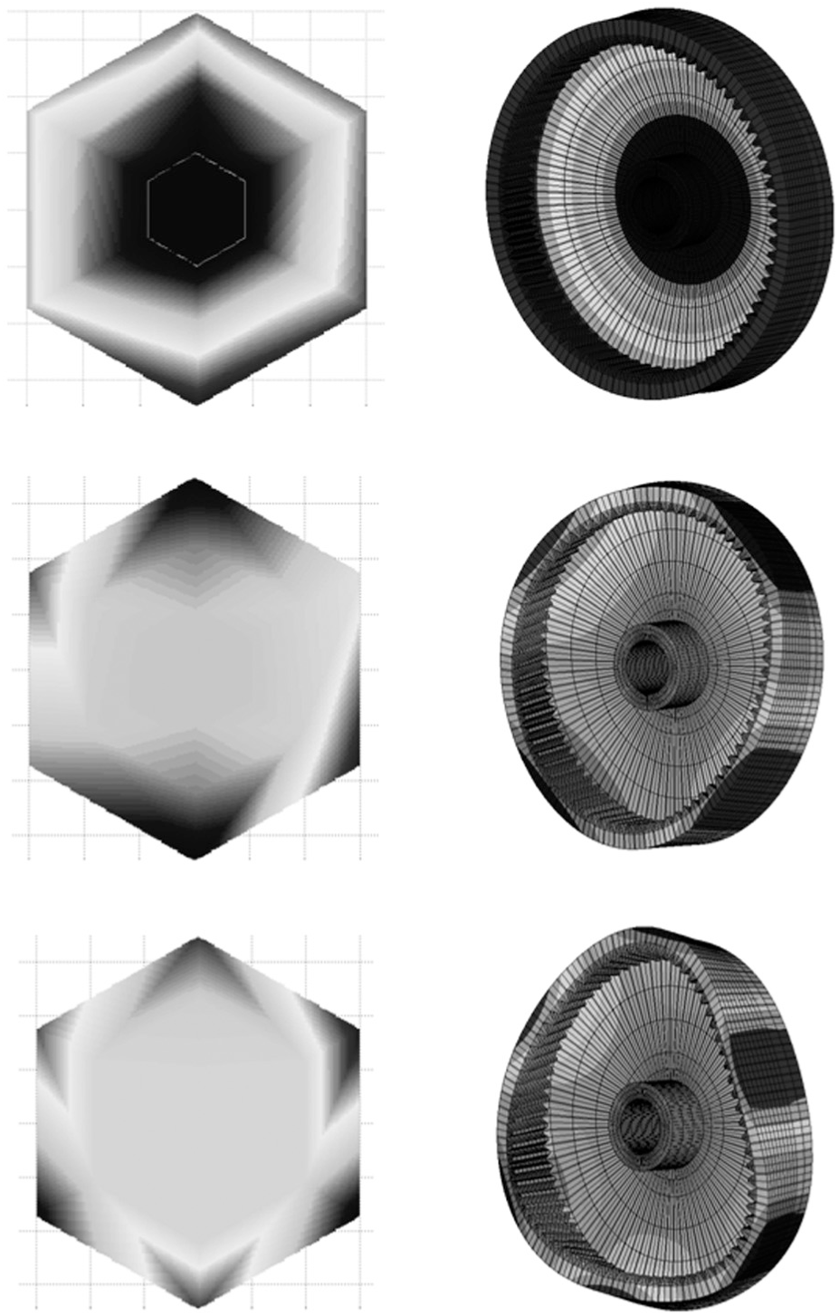
Three modes of vibration of the gear obtained by simulation (shown at right) and experimental tests (shown at left).

Conclusion

In this work, a methodology to create finite element models with high computational efficiency has been proposed. Although the methodology presents a general character, it has been introduced through the practical application to the modeling of two common mechanical devices: an optical linear encoder and a gear transmission, by means of its implementation in the parametric design language APDL. The methodology is supported over the current trends in the automatic generation of finite element models, like geometrical idealization, feature and detail removal, cell tessellation, dimensional reduction, and associativity maintenance, key concepts over which the methodology have been structured and sequenced. Additionally, the guidelines to model joining components such as compression and torsion springs, bearings, or adhesive joints by means of structural elements have also been presented. The application of the methodology lead to the creation of finite element models highly consistent with a minimal computational cost in the generation and analysis stages. Finally, the validity of the methodology has been verified through the comparison of the simulation results obtained with the finite element model with those obtained experimentally, being able to reproduce faithfully the modes of vibration of the encoder’s components and the gear transmission.