Sage Journals: Discover world-class research

Abstract

This study develops an integrated monitoring system with a human–machine interface (HMI) for groove grinding on the outer surface of the inner ring of a bearing type 6205 in an industrial environment. The proposed system is specifically designed to ensure stable real-time monitoring under progressive grinding wheel wear evolution, rather than maximizing prediction accuracy under fixed and stationary operating conditions. The system combines a grinding wheel wear measurement setup using pneumatic sensors, machine learning algorithms, and multi-objective optimization methods. The input data are collected in real time from the pneumatic measurement system (PMS) to monitor wheel wear ( $G_{w}$ ), and from inductive proximity sensors to count the number of processed parts ( $N_{p}$ ) in each grinding cycle. Subsequently, machine learning models (ANN, XGBoost, CatBoost, LightGBM) tuned with Bayesian optimization (BO) and combined with the NSGA-II algorithm are used to determine the optimal solutions for grinding conditions that consist of wheel feed rate ( $f_{w}$ ), workpiece speed ( $v_{w}$ ), depth of cut ( $a_{e}$ ), and $N_{p}$ , based on the objectives of maximizing material removal rate ( $Q_{w}$ ), and minimizing surface roughness ( $Ra$ ) and ovality ( $O_{p}$ ). The machine learning hyperparameters are optimized using the Bayesian algorithm. The selected solutions are adapted to user preferences and are used as input cutting parameters for the monitoring system. The SHapley Additive exPlanations (SHAP) technique is used to interpret the influence of grinding parameters on the output. The entire system is integrated into the HMI to display predictions in real time and to issue warnings when $Ra$ exceeds 0.3 µm, $O_{p}$ exceeds 3 µm, or $G_{w}$ exceeds 12 µm, at which point a dressing alert is triggered. In factory trials, the HMI maintained stable latency and prediction consistency, with MAPE values within 5% across the full wear range. These results reflect the actual behavior observed on the line and confirm that the system can operate reliably under industrial conditions.

Keywords

groove grinding real-time monitoring bearing machine learning multiobjective optimization

Introduction

Bearings are highly standardized products, coded and designed, manufactured, and tested according to international technical standards. This type of product is suitable for mass production and is widely used in industry. Control of the manufacturing process is necessary to ensure the accuracy, reliability, and performance of bearings.¹ The manufacturing process includes many stages, among which the outer groove grinding of the inner ring and the inner groove grinding of the outer ring using the centerless grinding method are highly complex and require strict technical precision, as these positions determine the bearing’s dimensional accuracy. Therefore, monitoring this process is truly necessary in large-scale mass production.²

Recently, many studies have focused on monitoring the grinding process to deal with recurring issues such as wheel wear, thermal damage, and the gradual change in product quality over a grinding cycle. Early approaches relied mainly on physical measurements—force, temperature, vibration, and acoustic emission (AE)—to infer surface quality and the state of the wheel. Shen³ applied AE sensors to assess grinding burn and grinding wheel life, while Feng et al.⁴ examined vibration responses to estimate surface characteristics. Yin et al.⁵ used pneumatic sensors to capture wheel–workpiece profiles and built an HMI for basic process visualization.

Building on these efforts, several studies have integrated multiple sensors with data-driven models. For instance, Pan et al.⁶ combined force and vibration signals, compressed them with PCA, and fed them into BP neural networks to track surface roughness trends during grinding. Kumar et al.⁷ relied on LabVIEW to trigger alarms for abnormal patterns in automotive grinding lines. Meanwhile, Lee et al.⁸ used grayscale features from CCD images with ANN models to estimate wheel wear, while Wang et al.⁹ predicted $Ra$ and $G_{w}$ from spindle power signals. These works broaden the sensing space, but the setups are still tied to single-task predictions and models that offer little transparency when deployed on production machines. More importantly, most frameworks stop at prediction; they rarely link model output to actionable adjustments that operators can actually use.

Stable operation in real industrial environments remains difficult for many sensor-based systems. Dust, coolant mist, grinding debris, and humidity fluctuations routinely interfere with signal quality, and this behavior has been reported across several machining processes. Pneumatic sensors, however, tend to maintain signal stability under these conditions and can achieve resolutions on the order of ±1 µm.^10,11 Proximity sensors also perform more reliably than optical sensors for workpiece counting in wet or contaminated environments.^12,13 Similar observations were noted in applications ranging from face milling of Grade 6 titanium alloy¹⁴ to drilling operations.¹⁵ In contrast, vibration, AE, and force signals often exhibited drift or loss of fidelity when coolant and debris accumulated on the machine. For this reason, PMS and proximity sensors were the only sources that stayed consistently reliable during long-term production testing, and the predictive models in this study were built around these measurements.

In addition, data-driven techniques have become increasingly important in grinding monitoring because they can capture nonlinear relations between multiple inputs—such as feed, speed, and depth of cut—and outputs such as $Ra$ , $G_{w}$ , and $Q_{w}$ .¹⁶ Several studies have shown that neural networks can predict surface finish with good accuracy,^17,18 and tree-based models have been particularly effective when the available dataset is small or unbalanced.¹⁹ LightGBM and CatBoost are now commonly used for their stability when dealing with highly nonlinear patterns.^20,21 In other words, ML is being used not only to estimate tool wear or surface quality, but also to reduce the operator’s workload by providing actionable predictions that can be incorporated into an HMI.

Despite these improvements, grinding remains a highly variable process, mainly because the behavior of the wheel changes continuously as wear progresses. As the wheel dulls, maintaining surface integrity becomes more difficult, which directly affects both roughness and dimensional accuracy.²² Many studies have reported a clear link between wheel wear and grinding performance, emphasizing the need for continuous monitoring and compensation.^23–25 This issue is even more pronounced in bearing-groove grinding, where high cutting forces accelerate wear and make the process sensitive to small parameter deviations. These characteristics explain why monitoring and adjusting the process in real time remains a practical requirement rather than an academic exercise.

Previous work has extensively analyzed the stability and geometric quality in grinding processes. Rowe²⁶ proposed methods to assess rounding mechanisms and dynamic stability charts in centerless grinding, highlighting process stability as a key factor influencing geometric error formation. Subsequent studies have examined profile evolution and roundness error during centerless grinding operations,²⁷ and investigated the effects of process parameters on workpiece roundness in bearing raceway grinding.²⁸ Analytical investigations into geometrical origins of roundness also exist,²⁹ and broader reviews on centerless grinding technology provide context on process dynamics and quality challenges.³⁰ In contrast, the present study focuses on in-process monitoring and data-driven evaluation of tool wear and performance indicators, complementing these earlier stability and roundness analyses.

Multi-objective optimization plays an increasingly important role in machining problems, especially when operators must handle conflicting targets such as reducing wheel wear while still maintaining a material removal rate high enough to satisfy production output. NSGA-II is one of the algorithms capable of handling this trade-off stably and has been applied in many machining studies.^31,32 These works show that NSGA-II can determine feasible operating parameter regions, particularly in grinding for automotive components. However, using NSGA-II directly on a production line is still limited because the algorithm requires high computational time and therefore decisions often suffer from noticeable latency. A more reasonable approach is using NSGA-II only to determine the optimal operating window before switching to the subsequent monitoring process.

In actual industrial grinding, an effective monitoring system cannot rely only on standalone sensors or standalone prediction models. A practical system must ensure three elements: (i) stable data acquisition under dust, coolant, and machine vibration; (ii) prediction models that do not collapse when operating conditions drift outside the training region; and (iii) real-time feedback presented through an interface that operators can use easily. Although multiple studies have addressed individual parts of this problem,^2–4 integrating them into a unified system that is reliable in production environments remains challenging.^16,33

The purpose of the monitoring system is to track tool wear progression and evaluate key grinding performance indicators during operation. The wear parameter $G_{we}$ is directly measured in-process, while predictive models are used to estimate selected performance outputs and support real-time warning. This enables timely dressing decisions and helps maintain surface quality and production stability in bearing ring grinding.

This study develops a monitoring framework based on PMS signals combined with machine-learning models, together with an NSGA-II optimization layer for the initial parameter-selection stage. The system provides direct visualization of predictions in real time and automatically warns when monitored values exceed technical limits. To enhance interpretability, SHAP is used to analyze the influence level of each input variable—something that machine operators often request when evaluating the reliability of a new monitoring tool. The overall workflow has five main steps: (1) collecting data under industrial conditions, (2) building and tuning models, (3) optimizing parameters with NSGA-II, (4) model-explanation analysis via SHAP, and (5) deploying and evaluating the HMI on the actual grinding line.

The final goal is to convert model predictions into operating decisions that operators can trust, especially in situations where wheel wear increases rapidly or where requirements for surface roughness and roundness become more stringent.³⁴ By relying on signals that remain stable in long-term operation and validating the system directly in production, this framework is designed to support immediate corrective actions instead of only providing offline analysis.

Materials and methods

Methodology flowchart

Experimental phase

The experiment was carried out directly on the grinding production line so that the data reflected the actual operating variations. Four input parameters were investigated, including $f_{w}$ , $v_{w}$ , $a_{e}$ , and $N_{p}$ —these are parameters that are frequently adjusted during groove grinding. In each cycle, PMS recorded $G_{we}$ and $G_{wt}$ . Surface roughness at the two positions ( ${Ra}_{we}$ , ${Ra}_{wt}$ ) was measured using a stylus profilometer; $O_{p}$ was measured using a D022 device; and $Q_{w}$ was calculated from the change in workpiece mass. These quantities matched the inspection criteria in the factory, making later usage convenient.

Data preprocessing and machine learning

After the data collection step, the dataset was reviewed and features showing duplicated or overlapping information were removed to keep the model compact and avoid redundancy. The cleaned dataset was then used to develop prediction models for the measured outputs using ANN, XGBoost, LightGBM, and CatBoost. Hyperparameters were tuned with Bayesian optimization, and model performance was evaluated using RMSE, MAE, and R² to select the surrogate models for the optimization stage.

Multi-objective optimization

The selected models were used as surrogate functions in the NSGA-II multi-objective optimization. The optimization problem was set up to find the parameter region that satisfies multiple conflicting objectives in groove grinding. The obtained Pareto set was used as the basis for determining operating parameters.

Model refinement and interpretability

In the refinement stage, the input set was updated to include additional information reflecting the change in grinding conditions over time. The prediction models were retrained with the expanded inputs, and the hyperparameters were adjusted again using Bayesian optimization.

To support interpretability, SHAP was applied to quantify the influence of each input variable on the predicted outputs, ensuring the models could be explained and validated during deployment in the monitoring system.

HMI development and validation

The HMI was constructed to integrate measured signals $G_{we}, G_{wt}, N_{p}$ together with predicted values of ${Ra}_{we}, O_{p}, Q_{w}$ . Warning thresholds were set according to technical requirements $G_{we}, G_{wt} > 12, {Ra}_{we} > 0.3, and O_{p} > 3$ .

The system was then brought to the production line to check its ability to operate under actual manufacturing conditions.

Figure 1 summarizes the complete workflow, encompassing data acquisition, model development and refinement, NSGA-II optimization, SHAP-based interpretation, and final HMI deployment.

Figure 1.

Methodological framework developed for real-time monitoring.

Experimental setup

The experimental setup was constructed to replicate the actual operating conditions of the groove-grinding stage used for finishing the inner-ring ball race of 6205 bearings (precision grade P5). This finishing operation governs the final geometry, surface finish, and roundness of the raceway. Supplemental Section 1 provides additional process details, and Supplemental Figure S2 includes the corresponding manufacturing drawings.

Prior to groove grinding, all inner rings were machined and inspected to meet dimensional and form tolerances. Only compliant workpieces were selected for experimentation, minimizing the copying effect inherent to centerless grinding.

Grinding trials were performed on a 3MK147B CNC groove-grinding machine. Figure 2 illustrates the main components involved in data acquisition: the workpiece, grinding wheel, workpiece feeding mechanism, proximity sensor, pneumatic probes positioned at the wheel top and wheel edge, profilometer probe, and ovality measurement device (D022). The roundness measurement device has a accuracy of 1 µm and was calibrated prior to experimentation. Considering that the specified roundness tolerance is 3 µm (Supplemental Figure S2), the measurement resolution is adequate to reliably evaluate form deviations. The workpieces were manufactured from AISI 52100 bearing steel, a material commonly used in bearing production because of its high hardness, wear resistance, and fatigue strength.³⁵ Material properties and chemical composition are listed in Supplemental Section 1.

Figure 2.

Experimental setup and data collection scheme: ① workpiece; ② grinding wheel; ③ workpiece feeding mechanism; ④ proximity sensor; ⑤ pneumatic probe at the wheel top; ⑥ pneumatic probe at the wheel edge; ⑦ machined inner ring ball race; ⑧ SJ-400 profilometer probe; ⑨ ovality measurement probe (D022); (I) position for assembly proximity sensor-details in Supplemental Section 1.

The grinding wheel used in the trials was an A100LV5 vitrified-bonded Al₂O₃ wheel (grit #100, medium grade, dense structure), a specification typically selected for precision grinding of hardened bearing steels. Prior to each experiment, the wheel was dressed to establish a consistent initial condition.

Accurate measurement of wheel wear during grinding was obtained using a PMS. Pneumatic gauging is well suited for industrial use due to its robustness, stability under coolant mist and debris, and its favorable resolution compared with optical or contact alternatives. In this study, wear was monitored at two locations— $G_{we}$ and $G_{wt}$ —each with an approximate resolution of 1 µm. The PMS arrangement followed the configuration described previously by Thang et al.¹¹ and summarized in Supplemental Section 1.

To ensure consistent indexing and reliable counting $N_{p}$ , two inductive cylindrical proximity sensors (Autonics PR12-4DP) were mounted parallel to the machine column. Inductive sensing was selected for its resistance to coolant, chips, and vibration, in addition to its low maintenance requirements and ease of integration in industrial environments.

Surface roughness at the wheel edge ${Ra}_{we}$ and ${Ra}_{wt}$ was measured after each grinding pass using a Mitutoyo Surftest SJ-400 stylus profilometer, following ISO 4287 with a cutoff length of 0.8 mm. $O_{p}$ of the inner-ring raceway was assessed using a D022 radial bearing comparator with 1 µm accuracy, following ISO 1101 guidelines. The PMS was calibrated before every trial, yielding repeatability of roughly ± 1 µm. All roughness and ovality measurements were repeated three times, and average values were used for analysis.

$Q_{w}$ was determined from the mass difference of each workpiece before and after grinding, measured on an analytical balance with ±0.01 g accuracy. The calculation followed:

Q_{w} = \frac{M_{before grinding} - M_{after grinding}}{T_{grinding process}}

(1)

The purpose of this work is process monitoring and multi-objective optimization under real production-line conditions, where mass measurement provides a direct and reliable performance indicator. Since the workpiece material (AISI 52100) has constant density throughout all experiments, conversion to volumetric MRR involves division by a constant value and does not affect the regression modeling, optimization procedure, or Pareto ranking.

The parameters $f_{w}, v_{w}, a_{e}$ and $N_{p}$ were varied systematically according to a factorial design, summarized in Table 1. The grinding wheel speed $v_{s}$ was kept constant at 60 m/s throughout all experiments. All secondary operating settings—rough-feed rate, and rough-grinding allowances—were kept constant throughout the study. To minimize environmental influences, all experiments were performed at a controlled temperature of 26 ± 1 °C and relative humidity of 65 ± 5%.

Table 1.

Experimental parameters and their values used in grinding trials.

Parameter	Symbol	Unit	Experimental Values
Fine feed rate	$f_{w}$	µm/s	5, 12.5, 20
Workpiece speed	$v_{w}$	m/min	6, 12, 18
Fine depth of cut	$a_{e}$	µm	10, 15, 20
Number of processed workpieces	$N_{p}$	-	10, 20, 30

Data collection and analysis

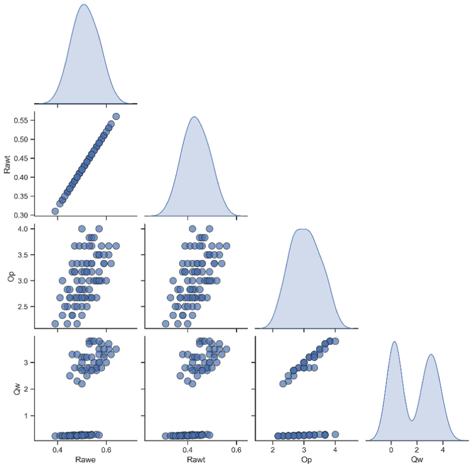
During each grinding trial, sensor readings and post-process measurements were gathered in parallel to capture how the process evolved from part to part. $G_{we}$ and $G_{wt}$ was recorded continuously through the PMS, while ${Ra}_{we}$ and ${Ra}_{wt}$ was measured after each pass. $O_{p}$ and $Q_{w}$ were also documented, reflecting the standard inspection routine used in bearing production. A complete summary of the experimental parameters is listed in Supplemental Table S5. Pairwise trends among the collected variables are illustrated in Figure 3.

Figure 3.

Pairplot visualization illustrating relationships among key output parameters: $G_{we}, G_{wt}$ , $R a_{we}, R a_{wt}$ , $O_{p}$ , and $Q_{w}$ .

Mass-based calculation was used to determine $Q_{w}$ , and roughness and ovality were measured using the same instruments described in the preceding section. These values were logged immediately after each part was processed, forming a continuous data series across the full sequence of trials.

Initial exploration of the dataset showed that the top-surface signals $G_{wt}$ and ${Ra}_{wt}$ varied only slightly and moved almost in parallel with the corresponding edge measurements. This behavior is visible in the comparative plots in Figure 4. Because these two variables contributed little additional information, they were removed from model development to avoid unnecessary dimensional overlap.

Figure 4.

Comparative plots of measured parameters across $N_{p}$ at $f_{w}$ = 12 µm/s, $v_{w}$ = 6 m/min, $a_{e}$ = 10 µm: (a) wheel wear ( $G_{we}$ and $G_{wt}$ ) and (b) surface roughness ( $R a_{we}$ and $R a_{wt}$ ).

Correlation heatmaps were then generated to examine the dependence between the remaining inputs and outputs. Prior to removing redundant variables, several groups of parameters appeared strongly clustered. After refinement, key dependencies—particularly those linking $G_{we}, N_{p},$ and $Q_{w}$ —became clearer (Figure 5). This cleaned structure served as the basis for later predictive modeling and optimization.

Figure 5.

Correlation heatmaps of experimental parameters: (a) before removal, and (b) after removal of redundant variables ( $G_{wt}, R a_{wt}$ ).

To further assess multicollinearity, Variance Inflation Factor (VIF) analysis was performed (Supplemental Material Section 4). The results show extremely high VIF values for ${Ra}_{we}$ (436.23) and ${Ra}_{wt}$ (291.35), as well as substantial multicollinearity for $G_{we}$ (33.76) and $G_{wt}$ (25.76). Combined with the strong Spearman correlation between the paired variables, these findings support the exclusion of $G_{wt}$ and ${Ra}_{wt}$ to avoid redundant information and improve model stability.

Machine learning models and tuning method

Four machine-learning algorithms—ANN, XGBoost, LightGBM, and CatBoost—were considered for predicting $G_{we}$ , ${Ra}_{we}$ , $O_{p}$ , and $Q_{w}$ . These models are widely used in machining studies because they can represent nonlinear effects without prescribing explicit functional forms.

Artificial neural networks (ANN)

ANNs provide flexible architectures capable of capturing nonlinear interactions. Their performance depends heavily on tuning and dataset quality, and interpretability may be limited.³⁶

Extreme gradient boosting (XGBoost)

XGBoost incorporates regularization and robust handling of noisy or incomplete data, making it suitable for manufacturing environments with natural variability.³⁷

Light gradient boosting machine (LightGBM)

LightGBM uses histogram-based feature binning and leaf-wise tree growth, offering fast training. Care is required when the dataset is modest in size, as the aggressive growth strategy may introduce overfitting.³⁸

Categorical boosting (CatBoost)

CatBoost handles ordered data effectively and mitigates prediction shift without heavy preprocessing. Training time is typically longer, but the model remains robust across many manufacturing-related tasks.³⁹

Tuning ML hyperparameters via BO

To enhance the predictive performance of the machine learning models employed in this research, hyperparameters were optimized using BO. Unlike conventional hyperparameter tuning methods such as grid search or random search, BO treats the hyperparameter tuning problem as the maximization of an unknown black-box objective function $F (x)$ , which maps a hyperparameter configuration $x$ to a validation performance measure (e.g. accuracy or error). The optimization goal is thus formulated as:

x^{*} = \arg \max_{x \in X} F (x),

(2)

where $X$ represents the feasible hyperparameter space.⁴⁰

BO builds a probabilistic surrogate—typically a Gaussian Process (GP)—to approximate $F (x)$ . The surrogate is updated after each evaluated configuration, and the next point $x_{n + 1}$ is chosen by maximizing an acquisition function $α_{n} (x)$ , which balances exploration and exploitation (Snoek et al., 2012).

A commonly used acquisition function is the Expected Improvement (EI), defined as:

{EI}_{n} (x) = E_{n} [\max (F (x) - f_{n}^{*}, 0)],

(3)

where $f_{n}^{*} = \max {F (x_{1}), \dots, F (x_{n})}$ is the best observed value after $n$ evaluations.¹⁹ Under a GP posterior, EI admits the closed-form expression:

\begin{matrix} {EI}_{n} (x) = (μ_{n} (x) - f_{n}^{*}) Φ (Z) + σ_{n} (x) ϕ (Z), \\ with Z = \frac{μ_{n} (x) - f_{n}^{*}}{σ_{n} (x)}, \end{matrix}

(4)

with $μ_{n} (x)$ and $σ_{n} (x)$ denoting the GP predictive mean and standard deviation, and $Φ (\cdot)$ , $ϕ (\cdot)$ being the CDF and PDF of the standard normal distribution.⁴¹

Data splitting and validation protocol

Because the grinding process is sequential and wheel wear accumulates progressively with increasing $N_{p}$ , the dataset (81 samples) was partitioned chronologically to prevent potential data leakage. The first 65 observations (80%), corresponding to early-cycle wear progression, were used for model training, while the remaining 16 samples (20%) from later-cycle stages were reserved for testing. The test dataset was strictly excluded from both model training and hyperparameter optimization. Hyperparameters were tuned using 5-fold cross-validation within the training dataset only. Final performance metrics (R², RMSE, and MAE) were computed exclusively on the held-out test set.

Model interpretability using SHAP values

SHAP analysis was applied to clarify how each input parameter influenced the model outputs. Rather than relying only on global feature rankings, SHAP provides contribution values for individual predictions, making it possible to trace which parameters increased or decreased the estimated responses. This type of interpretation is useful in machining studies, where the relative impact of feed rate, speed, depth of cut, or wear progression must be understood before model outputs can be used confidently on the production line.⁴² SHAP analysis was performed to interpret feature contributions. For tree-based models, TreeSHAP was applied. For the ANN model, SHAP values were computed using the KernelSHAP method to provide model-agnostic explanations.

Multiobjective algorithm

Optimal grinding conditions were determined using a multiobjective optimization procedure based on NSGA-II. The algorithm was used to explore combinations of the process parameters while accounting for the competing nature of the performance metrics.⁴³ The objectives were defined as:

Minimize: $G_{we}$ , ${Ra}_{we}$ , and $O_{p}$

Maximize: $Q_{w}$

Subject to the following input parameter constraints (Table 1):

5 \leq f_{w} \leq 20; 6 \leq v_{w} \leq 18; 10 \leq a_{e} \leq 20; 10 \leq N_{p} \leq 30

(5)

NSGA-II was chosen because of its reliability in handling engineering optimization tasks with nonlinear and conflicting criteria. The procedure maintains a diverse set of candidate solutions through fast nondominated sorting and crowding-distance selection, resulting in a Pareto front that reflects feasible trade-offs among wheel wear, surface quality, dimensional accuracy, and productivity.^44,45

HMI development

The HMI was designed to provide real-time visibility of the grinding process by combining live sensor readings with model-based predictions. The interface displays the measured $G_{we}$ , $N_{p}$ , and the predicted quality indicators— ${Ra}_{we}$ , $O_{p}$ , and $Q_{w}$ . The prediction module uses the suitable ML model, which was incorporated into the HMI due to its stable behavior during deployment and compatibility with continuous sensor input. To support on-line supervision, the HMI includes threshold-based alerts. When any monitored quantity exceeds its allowable limit: $G_{we}$ : >12 µm, ${Ra}_{we}$ : >0.3 µm, and $O_{p}$ : >3 µm.

The system highlights the deviation and prompts operator attention. These limits reflect technical requirements and early experimental observations. By presenting both measured and predicted values in a single interface, the HMI helps operators recognize process drift more quickly and intervene before out-of-tolerance conditions propagate through the production batch.

Results and discussion

Machine learning model optimization and evaluation

Four machine-learning models—ANN, XGBoost, CatBoost, and LightGBM—were tuned using Bayesian optimization. The final hyperparameter settings are listed in Supplemental Table S6. Model accuracy was evaluated with RMSE, MAE, and R². Figures 6 and 7 show the comparison across models for both the training and test datasets, with numerical values summarized in Table 2, where bold values indicate the best-performing model for each target and metric.

Figure 6.

Graphical comparison of RMSE, MAE, and R² among models predicting $G_{we}$ , ${Ra}_{we}$ , $O_{p}$ , and $Q_{w}$ in the training dataset.

Figure 7.

Graphical comparison of RMSE, MAE, and R² among models predicting $G_{we}$ , ${Ra}_{we}$ , $O_{p}$ , and $Q_{w}$ in the testing dataset.

Table 2.

Comparison of RMSE, MAE, and R² among models.

Model	Targets	Training dataset			Testing dataset
Model	Targets	RMSE	MAE	R ²	RMSE	MAE	R ²
ANN	$G_{we}$	0.8963	0.5160	0.7382	1.0396	0.8135	0.7098
XGBoost		0.0303	0.0226	0.9728	0.0334	0.0324	0.9529
CatBoost		0.0263	0.0196	0.9729	0.0273	0.0327	0.9630
LightGBM		0.5985	0.4805	0.9101	0.6647	0.6310	0.8803
ANN	${Ra}_{we}$	0.0192	0.0519	0.7095	0.0205	0.0685	0.6740
XGBoost		0.0049	0.0035	0.9675	0.0052	0.0041	0.9587
CatBoost		0.0057	0.0038	0.9654	0.0065	0.0045	0.9567
LightGBM		0.0069	0.0051	0.9616	0.0077	0.0076	0.9431
ANN	$O_{p}$	0.3096	0.2395	0.7845	0.3480	0.4081	0.7093
XGBoost		0.1950	0.1171	0.8991	0.2593	0.1735	0.8574
CatBoost		0.1958	0.1203	0.8783	0.2847	0.1766	0.8416
LightGBM		0.1967	0.1225	0.8830	0.2691	0.1853	0.8449
ANN	$Q_{w}$	0.7796	0.5005	0.7137	0.7796	0.6349	0.6852
XGBoost		0.3871	0.2751	0.9091	0.4059	0.3571	0.9055
CatBoost		0.3335	0.2251	0.9255	0.3917	0.3120	0.9070
LightGBM		0.5940	0.3974	0.8225	0.6207	0.4494	0.8233

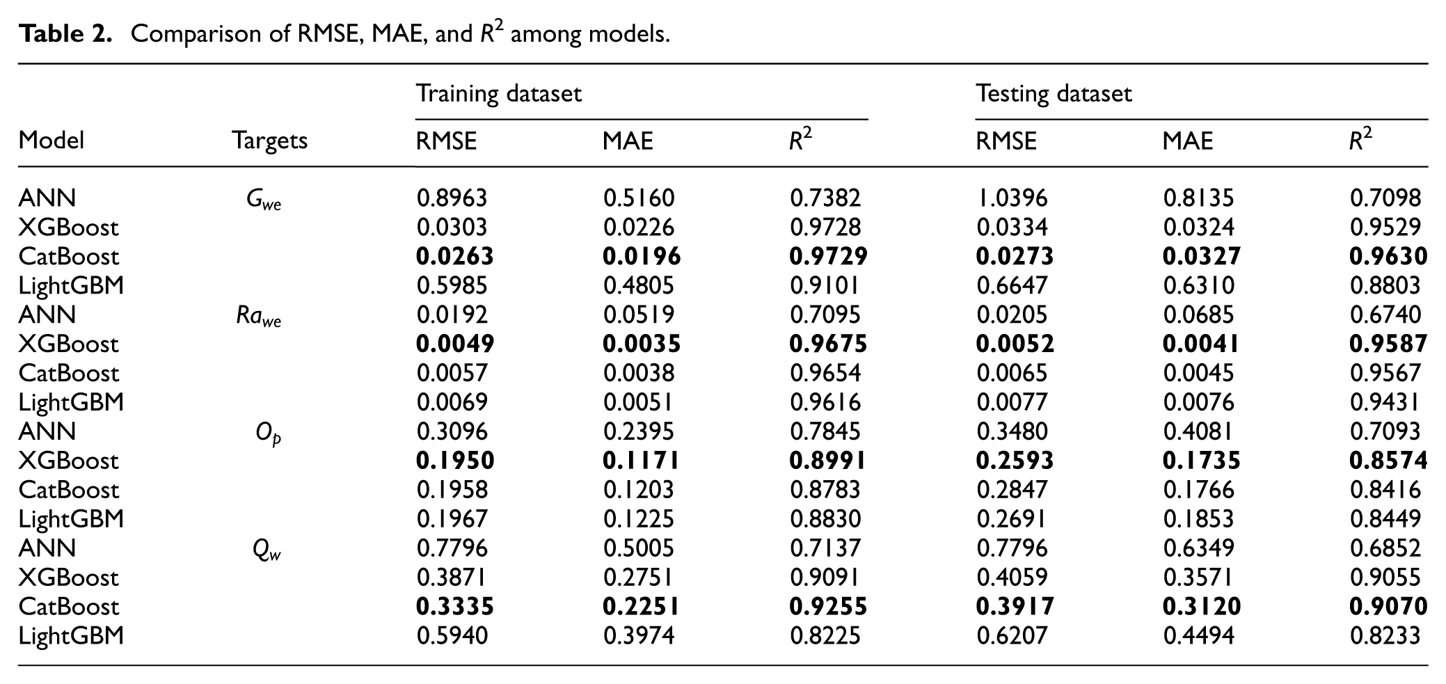
On the training set, CatBoost produced the lowest errors for $G_{we}$ with RMSE = 0.0263 and $Q_{w}$ with RMSE = 0.3335. While XGBoost provided the most accurate predictions for ${Ra}_{we}$ with RMSE = 0.0049, for $O_{p}$ XGBoost gave RMSE = 0.1950.

On the test set, CatBoost again performed best for $G_{we}$ and $Q_{w}$ , and XGBoost remained the most accurate model for ${Ra}_{we}$ and $O_{p}$ (see in Table 2).

From these results, the models selected for subsequent optimization were: $G_{we}$ , $Q_{w}$ is Catboost and ${Ra}_{we}$ , $O_{p}$ is XGBoost

These selected models were then used as surrogate functions in the multi-objective optimization stage.

Multi-objective optimization of grinding parameters

The previously selected optimal ML models were incorporated as objective functions into a multi-objective optimization framework using the NSGA-II algorithm. The NSGA-II approach successfully generated a set of Pareto-optimal solutions, effectively balancing competing objectives: minimizing $G_{we}$ , ${Ra}_{we}$ , and $O_{p}$ , while maximizing $Q_{w}$ . The complete results for 50 initial Pareto solutions are provided in Supplemental Table S7.

From these initial solutions, practical manufacturing constraints were applied to ensure industrial applicability:

Minimum $N_{p}$ : ≥15 parts per wheel dressing cycle.

${Ra}_{we}$ : ≤0.3 µm, from detailed bearing drawing specifications in Supplemental Figure S2.

$O_{p}$ : ≤3 µm, according to technical requirements in Supplemental Figure S2.

Applying these constraints reduced the Pareto-optimal set to 22 practical solutions, summarized clearly in Table 3. Table 3 explicitly provides recommended ranges for input parameters— $f_{w}$ , $v_{w}$ , $a_{e}$ , and $N_{p}$ —alongside predicted output values, enabling decision-makers to select optimal grinding conditions aligned with production requirements and practical constraints.

Table 3.

Practical Pareto-optimal input and output solutions derived from NSGA-II.

	Input parameters				Output parameters
	$f_{w}$	$v_{w}$	$a_{e}$	$N_{p}$	$G_{we}$	${Ra}_{we}$	$O_{p}$	$Q_{w}$
Solutions	µm/s	m/min	µm	part	µm	µm	µm	g/min
1	6.85	15.70	10.69	27	8.42	0.26	2.31	2.21
2	6.90	16.12	10.54	28	8.42	0.26	2.31	2.21
3	6.83	11.94	10.34	28	8.03	0.23	2.47	2.31
4	6.35	16.02	13.05	27	8.42	0.26	2.50	2.51
5	5.44	15.75	18.52	17	6.27	0.24	2.64	2.71
6	5.46	15.48	18.52	17	6.27	0.24	2.64	2.71
7	5.98	17.39	19.66	25	8.56	0.28	2.66	2.71
8	5.63	17.96	19.79	25	8.56	0.28	2.66	2.71
9	6.36	17.30	19.57	25	8.56	0.28	2.66	2.71
10	5.98	17.40	19.66	25	8.56	0.28	2.66	2.71
11	9.53	11.58	12.31	18	5.82	0.20	2.67	0.32
12	8.96	17.24	11.05	25	8.42	0.26	2.67	2.71
13	10.23	15.61	10.69	28	8.42	0.26	2.67	2.71
14	6.33	11.78	13.05	27	8.03	0.23	2.68	2.71
15	5.39	9.68	18.52	18	5.92	0.21	2.80	2.81
16	8.40	11.97	17.57	17	5.92	0.21	2.80	2.81
17	6.12	9.82	18.52	17	5.92	0.21	2.80	2.81
18	8.42	11.13	18.18	27	8.14	0.25	2.84	3.10
19	8.42	11.13	18.07	27	8.14	0.25	2.84	3.10
20	9.41	11.16	12.93	25	8.03	0.23	2.87	2.98
21	8.93	8.21	10.65	16	5.82	0.20	2.88	0.82
22	9.53	11.58	12.93	18	5.82	0.20	2.90	2.82
Max	10.23	17.96	19.79	28	8.56	0.28	2.90	3.10
Min	5.39	8.21	10.34	16	5.82	0.20	2.31	0.32

In Table 3, Solutions 5–6 and 7–10 correspond to different combinations of decision variables but produce identical objective values at the reported numerical precision. These solutions are distinct in the decision space but converge in the objective space. This behavior is consistent with multi-objective optimization, where locally low-sensitivity regions or discrete variables (e.g. $N_{p}$ ) may lead to similar objective outcomes. The full-precision objective values have been provided in Supplemental Table S7 to clarify this point.

Figure 8 visually illustrates these 22 selected solutions via a three-dimensional scatter plot, clearly depicting trade-offs among $G_{we}$ , ${Ra}_{we}$ , and $O_{p}$ , while color variation represents $Q_{w}$ . Such visualization effectively highlights the interplay among objectives, facilitating intuitive understanding and informed decision-making by operators and engineers.

Figure 8.

Visualization of Pareto-optimal solutions generated by the NSGA-II algorithm.

Input selection and predictive model refinement for HMI development

For real-time integration within the HMI, predictive accuracy alone is not sufficient; the model must also provide stable and consistent behavior during sequential monitoring as wheel wear progresses. Although CatBoost and XGBoost achieved slightly higher predictive accuracy in offline evaluation (Table 4), sequential monitoring tests revealed that the tree-based models exhibited locally discontinuous prediction behavior due to their piecewise structure.^46,47

Table 4.

Performance comparison of ANN models (with $G_{we}$ input) against best-performing previous models.

Model	Target	Training dataset			Testing dataset
ANN ( $G_{we}$ )	${Ra}_{we}$	0.0073	0.045	0.9871	0.0082	0.0051	0.9541
XGBoost	${Ra}_{we}$	0.0043	0.0034	0.9943	0.0046	0.0036	0.9843
ANN ( $G_{we}$ )	$O_{p}$	0.1122	0.0884	0.9439	0.1536	0.1187	0.8448
XGBoost	$O_{p}$	0.1725	0.1151	0.9241	0.2315	0.1509	0.8803
ANN ( $G_{we}$ )	$Q_{w}$	0.1827	0.0985	0.9842	0.0685	0.0369	0.9974
CatBoost	$Q_{w}$	0.2950	0.2213	0.9512	0.3497	0.2713	0.9312

Since the selected models function as surrogate predictors for continuous real-time tracking, stable responses to incremental changes in $N_{p}$ are desirable. In this context, the ANN model provided smoother and more consistent predictions during sequential operation.

In addition, the modeling framework was structured in two configurations for different purposes. In the optimization stage, surrogate models were trained using only controllable process parameters ( $f_{w}, v_{w}, a_{e}, N_{p}$ ) as inputs, while $G_{we}$ was treated as a target variable. This configuration allowed NSGA-II to explore feasible parameter regions based solely on adjustable process settings.

In the real-time monitoring stage, $G_{we}$ is directly measured online via the pneumatic measurement system and incorporated as an additional state variable for predicting ${Ra}_{we}$ , $O_{p}$ , and $Q_{w}$ . Under this configuration, $G_{we}$ is not used simultaneously as both input and output within the same model. All input variables correspond to quantities available at the time of prediction, ensuring that no future information is introduced.

The ANN incorporated $G_{we}$ together with the primary grinding parameters ( $f_{w}$ , $v_{w}$ , $a_{e}$ , $N_{p}$ ) to estimate $R_{awe}$ , $O_{p}$ , and $Q_{w}$ . Including $G_{we}$ improved representation of process evolution and cumulative wear effects.

As shown in Table 4, the ANN achieved predictive performance comparable to the best-performing tree-based models. Although XGBoost provided slightly higher offline accuracy for ${Ra}_{we}$ , the ANN maintained consistent behavior for $O_{p}$ and $Q_{w}$ during sequential monitoring. Figure 9 confirms stable convergence without signs of overfitting. Based on these results, the ANN model was integrated into the HMI for real-time prediction and process tracking.⁴⁸

Figure 9.

ANN model training history illustrating convergence and error stabilization for: (a) predicting $R a_{we}$ , (b) $O_{p}$ , and (c) $Q_{w}$ .

SHAP-based model interpretation

SHAP analysis was applied to the predictive models to examine how individual input parameters influenced each output. Because grinding wheel wear ( $G_{we}$ ) is itself a predicted variable, the CatBoost model for $G_{we}$ uses four inputs $(f_{w}, v_{w}, a_{e}, N_{p})$ . In contrast, the ANN models for ${Ra}_{we}$ , $O_{p}$ , and $Q_{w}$ incorporate five inputs, with $G_{we}$ included as an additional predictor due to its strong physical influence on surface and dimensional outcomes. This distinction explains why the SHAP plots differ in the number of variables considered.

Figure 10 summarizes the SHAP results for the wheel-wear model. Among the four inputs, the $N_{p}$ has the highest influence, followed by $f_{w}$ , $v_{w}$ , and $a_{e}$ . This trend aligns with established observations that wheel wear accumulates with repeated part engagement and is further shaped by feed and kinematic conditions.^7,49 The Beeswarm plot (Figure 10(b)) highlights that higher $N_{p}$ values consistently shift SHAP contributions upward, reflecting progressive wear throughout the grinding cycle.

Figure 10.

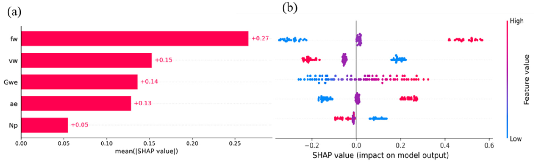
SHAP analysis for CatBoost prediction of grinding $G_{we}$ : (a) feature importance bar plot and (b) Beeswarm plot.

For surface roughness, the SHAP bar plot in Figure 11 shows that $G_{we}$ is the most influential parameter. Increased wear leads to higher roughness, consistent with machining studies reporting that cutting-edge degradation intensifies surface irregularities.^49,50 Other parameters ( $f_{w}, v_{w}, a_{e}, N_{p}$ ) contribute more modestly but still influence the predicted roughness, particularly at higher feed rates.

Figure 11.

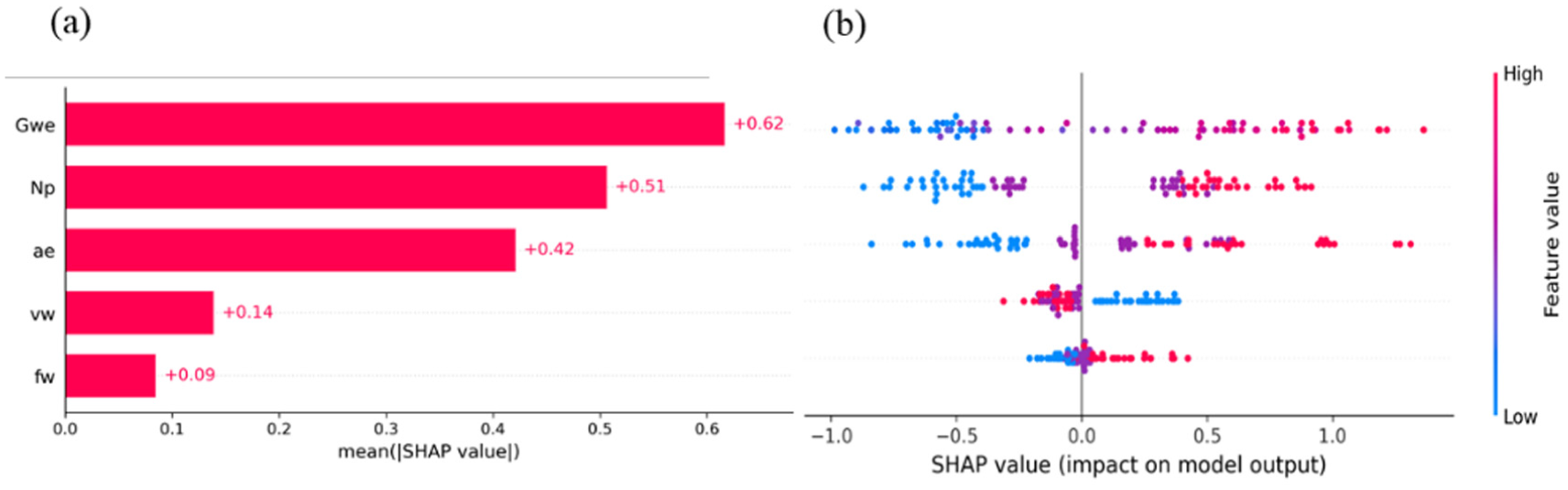
SHAP analysis for ANN prediction of $R a_{we}$ : (a) feature importance bar plot and (b) Beeswarm plot.

Figure 12 shows that wheel wear again dominates the SHAP distribution for ovality. As wear increases, the effective wheel profile deviates from its nominal geometry, producing measurable changes in groove roundness. This behavior aligns with machining principles in which tool condition plays a central role in dimensional accuracy.^2,51

Figure 12.

SHAP analysis for ANN prediction of $O_{p}$ : (a) feature importance bar plot and (b) Beeswarm plot.

For $Q_{w}$ , the SHAP analysis in Figure 13 identifies $a_{e}$ and $G_{we}$ as the two primary drivers. Higher depths increase chip load, while accumulated wear affects the effective contact area, both contributing to increased material removal.^35,49 The Beeswarm plot shows a clear positive shift in SHAP contributions for larger $a_{e}$ and higher wear states.

Figure 13.

SHAP analysis for ANN prediction of $Q_{w}$ : (a) feature importance bar plot and (b) Beeswarm plot.

HMI system and validation

The HMI used in this work was developed mainly to bring the sensor signals and the prediction models together in one place so that operators can follow the grinding process without switching between instruments. The interface layout in Figure 14 shows the three groups of information that the operators actually use on the shop floor.

Figure 14.

HMI layout showing: ① manual inputs ( $f_{w}$ , $v_{w}$ , $a_{e}$ ); ② real-time sensor measurements ( $N_{p}$ , $G_{we}$ , $G_{wt}$ ); ③ model-based predictions ( $R a_{we}$ , $O_{p}$ , $Q_{w}$ ); ④ real-time plot $G_{we}$ , $G_{wt}$ , $R a_{we}$ , $O_{p}$ ; ⑤ and threshold-based alerts.

Input parameters

Operators still enter $f_{w}$ , $v_{w}$ , and $a_{e}$ manually at the beginning of each run. These values usually come from the recommended ranges obtained from the earlier optimization results from Table 3, but in practice they may adjust slightly depending on material batches or wheel condition. Meanwhile, $N_{p}$ is read directly from the proximity sensors, and the pneumatic probes continuously supply $G_{we}$ and $G_{wt}$ . These readings arrive at short intervals and form the basis for all subsequent predictions.

Real-time predictions and visualization

Whenever new sensor values appear, the HMI refreshes the predicted ${Ra}_{we}$ , $O_{p}$ , and $Q_{w}$ .The small line plots beside each value help the operator check whether the process is drifting. In daily use this is often more useful than the numeric value itself because the drift usually shows up earlier than the threshold crossing.

Alerts and limits

Warnings are triggered when any of the following are exceeded:

$G_{we}$ or $G_{wt}$ >12 µm

${Ra}_{we}$ > 0.3 µm

$O_{p}$ > 3 µm

The alarm thresholds are derived from the design tolerances specified in the technical drawing of the 6205 inner bearing ring (Supplemental Figure S2). In particular, the roundness limit (≤0.003 mm) and surface roughness requirement ( ${Ra}_{we}$ ≤0.30 µm) correspond directly to the component’s geometric tolerance specifications.

On the actual HMI, the warning panel flashes and requires operator acknowledgment, reducing the risk of missing a necessary dressing operation.

Industrial validation

The interface was tested directly on the production line under three operating conditions selected from Table 3. Each condition was repeated three times. The comparison between measured and predicted values for ${Ra}_{we}$ , $O_{p}$ , and $Q_{w}$ is shown in Table 5 using MAPE.

Table 5.

Validation and predictive accuracy metrics (MAPE) of the HMI system.

Sols	Test	${Ra}_{we}$			$O_{p}$			$Q_{w}$
Sols	Test	Measured	HMI	APE (%)	Measured	HMI	APE (%)	Measured	HMI	APE (%)
5	1	0.27	0.257	6.20%	2.24	2.462	9.91%	2.31	2.382	3.10%
5	2	0.25	0.263	5.20%	2.25	2.494	10.84%	2.25	2.320	3.10%
5	3	0.27	0.260	4.41%	2.24	2.368	5.71%	2.34	2.275	2.78%
11	1	0.25	0.243	3.57%	2.64	2.651	0.40%	0.34	0.355	4.84%
11	2	0.25	0.252	0.80%	2.73	2.646	3.09%	0.39	0.412	4.73%
11	3	0.24	0.238	0.83%	2.72	2.740	0.74%	0.43	0.397	7.89%
22	1	0.24	0.241	0.42%	2.85	2.982	4.63%	2.71	2.874	6.04%
22	2	0.26	0.254	2.31%	2.74	2.845	3.83%	2.81	2.775	1.26%
22	3	0.26	0.265	1.92%	2.96	2.969	0.30%	2.95	2.834	3.97%
MAPE		2.85%			4.39%			4.19%

In most cases the prediction error stayed below about 5%. The deviations were small enough that the operator could rely on the displayed values without double-checking every part. This also confirmed that the ANN-based models remained stable when connected to the real sensors and running continuously for several hours.

The current validation focused on short runs to check that the system responds quickly and follows the main trends. However, in real production, operators run the line for many hours and through multiple dressing cycles. A longer continuous test is still needed to observe drift and to add simple confidence indicators so operators know how much they can trust each prediction during long shifts.

Recommendations for future enhancements

A few additions could make the system more stable in daily use. Extra signals such as vibration or temperature would help capture process changes that the pneumatic probes alone may miss.⁵² Another practical step is adding a simple adaptive or feedback mechanism so the system can adjust certain parameters without waiting for manual input, which has been shown to reduce inconsistency in similar setups.⁵³

At the current stage, the HMI already combines the key measurements and predictions on one screen, giving operators a clear picture of the process and when corrections are needed. Future improvements would mainly focus on reducing operator workload and keeping the system steady even when conditions vary.

Deployment considerations and limitations

Despite significant advances demonstrated by the proposed predictive framework and integrated HMI system, several critical factors and limitations should be carefully addressed before practical industrial deployment.

Firstly, the reliability of trained machine learning models heavily depends on the similarity of new operational conditions to the original experimental scenarios used for model training. Extending these predictive models beyond their original operational domain—such as substantially different machining parameters or alternative workpiece materials—may lead to decreased accuracy or even model invalidation. This inherent limitation in supervised machine learning models underscores the necessity of periodic retraining or adaptive updates, particularly when substantial shifts in machining conditions or materials occur.^54,55

Secondly, the effectiveness of the integrated sensor system depends on careful calibration, maintenance, and synchronization. Specifically, PMS is used for measuring wheel wear ( $G_{we}$ , $G_{wt}$ ) require regular calibration and maintenance to maintain measurement resolution and accuracy (±1 µm). Practical challenges related to sensor drift, misalignment, and contamination sensitivity on the shop floor must be managed through routine inspection and recalibration procedures.⁵⁶ Similarly, the proximity sensors monitor the number of processed parts ( $N_{p}$ ) should be adequately protected from environmental disturbances such as dust accumulation and mechanical vibrations to maintain precise data acquisition.

Finally, real-time latency is another point to keep in view. The current HMI responds in under 0.5 s, which is sufficient for the present setup, but production lines with higher throughput may demand faster updates. In such cases, moving the inference step to an edge device or a small embedded controller could reduce delays and avoid reliance on a central PC.⁵⁷

Although SHAP helps explain model behavior, it does not eliminate the black-box character of ML models. For this reason, the interface should present warnings and visual cues in a way that operators can interpret quickly, as noted by Nian⁵⁸ regarding effective adoption of ML tools on the shop floor.

The method in this study was developed for groove grinding of bearing inner rings. Applying it to other grinding tasks would likely require adjustments to reflect different workpiece shapes, fixturing, or material responses. In some cases, retraining or transfer learning may be needed.

There are also practical considerations for long-term use: sensor robustness, how often the model should be refreshed, and whether the interface remains simple enough for daily operation. Future versions may also link to MES or SCADA systems or support basic adaptive control and predictive-maintenance functions.

In this study, the models were trained and tested on a single wheel batch and a fixed machine setup. This helps keep the tests consistent, but of course it does not cover every production scenario. In actual factories, wheels, materials, and machine conditions vary from batch to batch. We plan to test the system across different wheels and longer production shifts to make sure the model stays stable under real production changes.

Conclusion

The work in this study was carried out to understand how a monitoring system could actually run on a groove-grinding line, not only under lab conditions. A few points came out clearly during the tests.

First, the pneumatic probes and the proximity sensors behaved much more consistently than other sensing options we tried earlier. This is not new in theory, but in our case the data showed that $G_{wt}$ and ${Ra}_{wt}$ carried little usable variation. Removing them made the models less noisy and also matched the real behavior of the wheel: the edge section deteriorates earlier and dominates quality issues.

Second, although tree-based models (CatBoost, XGBoost) gave the best numerical accuracy in the training domain, they became unstable when $N_{p}$ went outside the experimental range. This issue only appeared during live testing, not in cross-validation. The ANN handled this drift better once $G_{we}$ was included as an input. This was an important practical finding, as it determined which model type could run inside the HMI.

Third, the multi-objective optimization produced parameter windows that the operators felt were reasonable, not just mathematically optimal. The solutions meeting ${Ra}_{we} \leq 0.3$ µm and $O_{p} \leq 3$ µm matched what the factory already aims for. The output range for $Q_{w}$ under these constraints also helped clarify where the wheel deterioration starts affecting productivity.

The HMI, once integrated, was able to show wear, roughness and ovality predictions with errors generally below 5%. During long shifts, operators reported that the early-warning behavior (especially for $G_{we}$ ) helped them anticipate dressing earlier, instead of waiting until a part failed inspection. This observation is small but meaningful, because it suggests the system is usable even without full automation.

Overall, the study indicates that a practical monitoring tool for groove grinding must combine:

(1) sensors that actually survive coolant and dust,

(2) models that remain stable when operating conditions drift, and

(3) a simple interface that lets the operator react quickly.

Future work will verify the optimized parameter ranges under more operating conditions and different wheel states. This will help confirm how well the optimization works on the line and make the system easier to apply in day-to-day production.

Supplemental Material

sj-docx-1-ade-10.1177_16878132261442324 – Supplemental material for In-process tool wear and performance parameters monitoring for real-time warning during groove grinding bearing production

Supplemental material, sj-docx-1-ade-10.1177_16878132261442324 for In-process tool wear and performance parameters monitoring for real-time warning during groove grinding bearing production by Anh-Tuan Nguyen and Van-Hai Nguyen in Advances in Mechanical Engineering

Footnotes

Appendix

Acknowledgements

The authors gratefully acknowledge the Pho Yen bearing manufacturing facility for supporting data acquisition and for permitting real-time deployment and evaluation of the proposed monitoring system on their production line.

Handling Editor: Rahul Davis

ORCID iD

Van-Hai Nguyen

Author Contributions

Anh-Tuan Nguyen: Conceptualization, Methodology, Experimental investigation, Data curation, Writing—original draft. Van-Hai Nguyen: Supervision, Validation, Formal analysis, Writing—review & editing.

Funding

This research was supported by the Ministry of Science and Technology of Vietnam under project registration number 2024-24-0302/NS-KQNC.

Declaration of conflicting interests

The authors declared no potential conflicts of interest with respect to the research, authorship, and/or publication of this article.

Data availability statement

The data supporting the findings of this study are available from the corresponding author upon reasonable request.*

Supplemental material

Supplemental material for this article is available online.

References

Ding

, et al. A review of bearing failure modes, mechanisms and causes. Eng Fail Anal 2023; 152: 107518.

Kishore

Sinha

Singh

, et al. A comprehensive review on the grinding process: advancements, applications and challenges. Proc IMechE, Part C: J Mechanical Engineering Science 2022; 236: 10923–10952.

Shen

C-H

. Acoustic emission based grinding wheel wear monitoring: Signal processing and feature extraction. Appl Acoust 2022; 196: 108863.

Feng

Ding

Qiao

, et al. Correlation between vibration signal and surface quality based on recurrence analysis during surface burnishing process. Mech Syst Signal Process 2023; 200: 110654.

Yin

Nguyen

Chen

, et al. Application of compressed air in the online monitoring of surface roughness and grinding wheel wear when grinding Ti-6Al-4V titanium alloy. Int J Adv Manuf Technol 2019; 101: 1315–1331.

Pan

Qiao

Wang

, et al. Real-time prediction of grinding surface roughness based on multi-sensor signal fusion. Int J Adv Manuf Technol 2023; 127: 5847–5861.

Kumar

Park

Nedelcu

. Development of real-time grinding process monitoring and analysis system. Int J Precis Eng Manuf 2021; 22: 1345–1355.

Lee

Fan

Sencer

. Real-time grinding wheel condition monitoring using linear imaging sensor. Procedia Manuf 2020; 49: 139–143.

Wang

Tian

Zhang

, et al. Online prediction of grinding wheel condition and surface roughness for the fused silica ceramic composite material based on the monitored power signal. J Mater Res Technol 2023; 24: 8053–8064.

10.

Tanaka

Koshy

. A pneumatic sensor for grinding wheel condition monitoring. Precis Eng 2019; 56: 62–68.

11.

Thang

Tuan

Tiep

. Evaluation of grinding wheel wear in wet profile grinding for the groove of the ball bearing’s inner ring by pneumatic probes. J Mech Sci Technol 2018; 32: 1297–1305.

12.

Moheimani

Hosseini

Mohammadi

, et al. Recent advances on capacitive proximity sensors: from design and materials to creative applications. C 2022; 8: 26.

13.

Panda

Panigrahi

Mishra

, et al. Robotics for general material handling machines in food plants. In: Jafari

Malekjani

(eds) Transporting operations of food materials within food factories. Elsevier, 2023, pp. 341–372.

14.

Toprak

İB

Çolak

Bayhan

. Determination of the tool wear using cutting force in face milling of Ti-6Al-4V under high pressurized cooling conditions. El-Cezeri 2024; 11: 82–93.

15.

Cheong

ACH

Jie

Xian

JIYY

, et al. Digital twin in manufacturing by using programmable logic controller (PLC). AIP Conf Proc 2023; 2643: 050021.

16.

Ördek

Borgianni

Coatanea

. Machine learning-supported manufacturing: a review and directions for future research. Prod Manuf Res 2024; 12: 2326526.

17.

Dehghanpour Abyaneh

Narimani

Javadi

, et al. Predicting surface roughness and grinding forces in UNS S34700 steel grinding: a machine learning and Genetic algorithm approach to coolant effects. Physchem 2024; 4: 495–523.

18.

Nguyen

. Developing geometric error compensation software for five-axis CNC machine tool on NC program based on artificial neural network. In: Khang

Hoang

Ceccarelli

(eds) Advances in Asian mechanism and machine science. Springer International Publishing, 2022, pp. 541–548.

19.

Nguyen

V-H

T-T

Truong

H-S

, et al. Applying Bayesian optimization for machine learning models in predicting the surface roughness in single-point diamond turning polycarbonate. Math Probl Eng 2021; 2021: 1–16.

20.

Ren

Wang

Pang

, et al. Modeling and monitoring the material removal rate of abrasive belt grinding based on vision measurement and the gene expression programming (GEP) algorithm. Int J Adv Manuf Technol 2022; 120: 385–401.

21.

Nguyen

V-H

T-T

. Predicting surface roughness in machining aluminum alloys taking into account material properties. Int J Comput Integr Manuf 2025; 38: 555–576.

22.

Qin

Liu

Cheng

, et al. Study on wear mechanism of small ball-end grinding wheel and surface integrity of complex component under high-speed machining condition. Wear 2025; 570: 205907.

23.

Wan

Chen

Zhang

, et al. A multi-sensor monitoring methodology for grinding wheel wear evaluation based on INFO-SVM. Mech Syst Signal Process 2024; 208: 111003.

24.

Safarzadeh

Leonesio

Bianchi

, et al. Roundness prediction in centreless grinding using physics-enhanced machine learning techniques. Int J Adv Manuf Technol 2021; 112: 1051–1063.

25.

Bosso

Magelli

Zampieri

. Simulation of wheel and rail profile wear: a review of numerical models. Railw Eng Sci 2022; 30: 403–436.

26.

Rowe

. Rounding and stability in centreless grinding. Int J Mach Tools Manuf 2014; 82–83: 1–10.

27.

Yan

Fan

, et al. Profile evolution and cross-process collaboration strategy of bearing raceway by centerless grinding and electrochemical mechanical machining. Micromachines 2022; 14: 63.

28.

Tuan

. The effects of process parameters on workpiece roundness in the shoe-Type centerless grinding operation for internal raceway of ball bearings. Coatings 2023; 13: 1864. https://doi.org/10.3390/coatings13111864

29.

Cui

Ding

Cheng

. An analytical investigation on the workpiece roundness generation and its perfection strategies in centreless grinding. Proc IMechE, Part B: J Engineering Manufacture 2015; 229: 409–420.

30.

Hashimoto

Gallego

Oliveira

JFG

, et al. Advances in centerless grinding technology. CIRP Ann 2012; 61: 747–770.

31.

Verma

Pant

Snasel

. A comprehensive review on NSGA-II for multi-objective combinatorial optimization problems. IEEE Access 2021; 9: 57757–57791.

32.

Wang

Tian

, et al. Predictive modelling and Pareto optimization for energy efficient grinding based on aANN-embedded NSGA II algorithm. J Clean Prod 2021; 327: 129479.

33.

Rihi

Baïna

Mhada

, et al. Predictive maintenance in mining industry: grinding mill case study. Procedia Comput Sci 2022; 207: 2483–2492.

34.

Bántay

Abonyi

. Machine learning-supported designing of human–machine interfaces. Appl Sci 2024; 14: 1564.

35.

Rowe

. Principles of modern grinding technology. William Andrew, https://books.google.com/books?hl=vi&lr=&id=FRI3AgAAQBAJ&oi=fnd&pg=PP1&dq=Rowe,+W.+B.+(2013).+Principles+of+Modern+Grinding+Technology&ots=J0vfvE4EA2&sig=MzLHuwicZU-8GUzMi2yF9K89V3E (2013, accessed 23 March 2025).

36.

Huang

Chen

. Comparison of different machine learning algorithms for predicting the SAGD production performance. J Pet Sci Eng 2021; 202: 108559.

37.

Alizamir

Wang

Ikram

RMA

, et al. An interpretable XGBoost-SHAP machine learning model for reliable prediction of mechanical properties in waste foundry sand-based eco-friendly concrete. Results Eng 2025; 25: 104307.

38.

Meng

Finley

, et al. Lightgbm: a highly efficient gradient boosting decision tree. Adv Neural Inf Process Syst 2017; 30: 3149–3157.

39.

Dorogush

Ershov

Gulin

. CatBoost: gradient boosting with categorical features support. ArXiv Preprint ArXiv181011363, 2018.

40.

Brochu

Cora

de Freitas

. A tutorial on Bayesian optimization of expensive cost functions, with application to active user modeling and hierarchical reinforcement learning. Epub ahead of print 12 December 2010. https://doi.org/10.48550/arXiv.1012.2599.

41.

Frazier

. A tutorial on Bayesian optimization. Epub ahead of print 8 July 2018. https://doi.org/10.48550/arXiv.1807.02811.

42.

Rodemann

Croppi

Arens

, et al. Explaining Bayesian optimization by Shapley values facilitates human-AI collaboration. Epub ahead of print 8 March 2024. https://doi.org/10.48550/arXiv.2403.04629.

43.

Deb

Pratap

Agarwal

, et al. A fast and elitist multiobjective genetic algorithm: NSGA-II. IEEE Trans Evol Comput 2002; 6: 182–197.

44.

You

Han

Tian

, et al. Multi-objective optimization of grinding process parameters for improving gear machining precision. J Central South Univ 2025; 32: 538–551–https://doi.org/10.1007/s11771-025-5877-7

45.

Thapliyal

Kumar

. Comprehensive performance metric for bio-inspired optimizers: a generation-wise population convergence approach toward global optimality. Iran J Comput Sci 2025; 8: 843–891–https://doi.org/10.1007/s42044-025-00245-9

46.

Géron

. Hands-on machine learning with Scikit-Learn, Keras, and TensorFlow. O’Reilly Media, Inc, 2022.

47.

Rudin

. Stop explaining black box machine learning models for high stakes decisions and use interpretable models instead. Nat Mach Intell 2019; 1(5): 206–215.

48.

Zhang

Huang

, et al. An effective convolutional neural network based on SMOTE and Gaussian mixture model for intrusion detection in imbalanced dataset. Comput Netw 2020; 177: 107315.

49.

Deresse

Deshpande

Taifa

IWR

. Experimental investigation of the effects of process parameters on material removal rate using Taguchi method in external cylindrical grinding operation. Eng Sci Technol Int J 2020; 23: 405–420.

50.

Tuan

. Multi-objective optimization of process parameters to enhance efficiency in the shoe-type centerless grinding operation for internal raceway of ball bearings. Metals 2021; 11: 893.

51.

Malkin

Guo

. Grinding technology: theory and application of machining with abrasives. Industrial Press Inc., https://books.google.com/books?hl=vi&lr=&id=l3260ZF_PfQC&oi=fnd&pg=PP11&dq=Malkin,+S.,+%26+Guo,+C.+(2008).+Grinding+Technology:+Theory+and+Applications+of+Machining+with+Abrasives+&ots=V64yaD6XgR&sig=fbxq25zYb6BbzWm6Qlq3wdZBI24 (2008, accessed 23 March 2025).

52.

Kuntoğlu

Salur

Gupta

, et al. A state-of-the-art review on sensors and signal processing systems in mechanical machining processes. Int J Adv Manuf Technol 2021; 116: 2711–2735.

53.

Pervez

Ahamed

Ahmed

, et al. Autonomous grinding algorithms with future prospect towards SMART manufacturing: a comparative survey. J Manuf Syst 2022; 62: 164–185.

54.

Wuest

Weimer

Irgens

, et al. Machine learning in manufacturing: advantages, challenges, and applications. Prod Manuf Res 2016; 4: 23–45.

55.

Derakhshan

Mahdiraji

Rabl

, et al. Continuous deployment of machine learning pipelines. In: EDBT, 2019, pp.397–408.

56.

Kannan

Arunachalam

Chawla

, et al. Multi-sensor data analytics for grinding wheel redress life estimation - an approach towards industry 4.0. Procedia Manuf 2018; 26: 1230–1241.

57.

Haricha

Khiat

Issaoui

, et al. Recent technological progress to empower smart manufacturing: review and potential guidelines. IEEE Access 2023; 11: 77929–77951.

58.

Nian

. Machine learning for industrial processes: prediction, monitoring, and adaptive control, https://era.library.ualberta.ca/items/101390d9-2390-40aa-a83a-42546b0e4a79 (2020, accessed 25 March 2025).

Supplementary Material

Please find the following supplemental material available below.

For Open Access articles published under a Creative Commons License, all supplemental material carries the same license as the article it is associated with.

For non-Open Access articles published, all supplemental material carries a non-exclusive license, and permission requests for re-use of supplemental material or any part of supplemental material shall be sent directly to the copyright owner as specified in the copyright notice associated with the article.

1.63 MB

0.00 MB