
Abstract
To address the low accuracy and poor robustness of anomaly detection for planetary gear trains under asymmetric sample conditions, this paper proposes a generalized generative adversarial network (GGAN) method. The proposed approach integrates a generative adversarial network, an autoencoder, and a contrastive learning mechanism. By leveraging a multi-scale discriminator and a residual network to extract nonlinear feature discrepancies, and combining kernel density estimation to quantify anomaly probabilities, it significantly improves anomaly detection accuracy. Building on the GGAN-based anomaly detection method, a three-stage anomaly evaluation framework is developed. In the normal operation stage, the initial detection model is trained using only normal samples. In the early degradation stage, the detection threshold and model parameters are refined using a limited number of anomalous samples. In the severe degradation stage, multi-scenario data fusion and similarity analysis are incorporated to achieve robust evaluation. Experimental results demonstrate that the proposed method can provide theoretical support and practical reference for research and applications in related fields.
Introduction
As a core component of the transmission systems in large-scale complex equipment such as helicopter main reducers, shield tunneling machines, and wind turbine gearboxes, the operating condition of planetary gear sets directly determines the safety and reliability of the entire machine.1–4 Due to their frequent operation under harsh working conditions, planetary gear sets are highly susceptible to progressive faults such as fatigue pitting and tooth breakage.5–7 The evolution of these faults typically exhibits distinct stage-wise characteristics,8,9 progressing from normal operation through imperceptible initial degradation, and ultimately developing into severe degradation that may lead to catastrophic consequences. Therefore, achieving early and accurate anomaly detection of the multi-stage degradation process in planetary gear sets holds significant engineering value for implementing predictive maintenance, preventing unplanned downtime, and ensuring the safety of personnel and equipment.
However, in practical industrial scenarios, obtaining comprehensive and balanced abnormal state data poses significant challenges. Equipment operates in a healthy state for the vast majority of its lifecycle, resulting in an extreme scarcity of abnormal samples available for training-particularly those representing subtle fault signatures characteristic of the initial degradation stage. This issue of “imbalanced data,” where the number of “normal” and “abnormal” samples is severely unbalanced, is one of the core bottlenecks currently faced by intelligent fault diagnosis methods.10,11 Traditional deep learning-based anomaly detection models heavily rely on large-scale, high-quality training data. 12 Under imbalanced sample conditions, these models tend to misclassify the scarce abnormal samples as the majority normal state, leading to a sharp increase in the false negative rate and a severe deficiency in early degradation detection capability. 13 Furthermore, the structural complexity of planetary gear sets (such as complex vibration signal transmission paths and significant modulation phenomena) and the time-varying nature of operating conditions further exacerbate the difficulty of extracting condition features and discriminating abnormalities. 14 Consequently, developing a robust anomaly detection model that can accurately capture early degradation and strongly discriminate among different fault stages under severe class-imbalance conditions has become a key scientific problem that urgently needs to be addressed in this field.
In recent years, deep learning-based anomaly detection methods have gradually attracted increasing attention. Among these, techniques such as autoencoders (AE), generative adversarial networks (GAN), and their variants have demonstrated excellent performance in the field of anomaly detection.15–17 A deep learning-based fault diagnosis method for generators was introduced, significantly improving the accuracy of fault identification. 18 Subsequently, a deep learning-driven fault diagnosis model for transmission chains was developed, further advancing the level of intelligence in fault diagnosis. 19 Additionally, convolutional neural networks were employed to diagnosis bearing faults under multiple load conditions. 20 Due to their superior performance under small-sample conditions, GAN models have drawn growing interest from researchers in recent years. GANs were first introduced by Goodfellow and initially applied in the field of image generation. When trained on a specific dataset, a GAN model learns to generate new data that share the same statistical distribution as the original dataset. A gear fault diagnosis method based on conditional generative adversarial networks was proposed, which enhanced the model’s generalization ability and improved diagnostic accuracy by generating fault data under different operating conditions. 21 A comprehensive review was conducted on the application of artificial intelligence in rotating machinery fault diagnosis, highlighting the potential of GANs in fault data generation and data augmentation, thereby pointing toward future research directions. 22 Furthermore, a rolling bearing fault diagnosis method combining GAN and convolutional neural networks was presented, where GANs were used to generate fault data and CNNs were applied for feature extraction and fault classification, leading to improved diagnostic accuracy. 23
However, despite these advances, the existing literature still exhibits notable gaps, particularly in the context of progressive fault degradation and severe class imbalance. Most current GAN-based diagnostic models focus on fault detection under relatively balanced or controlled sample conditions, while insufficient attention has been paid to their performance under dynamically shifting class distributions – a common scenario in real-world industrial degradation processes. Furthermore, while GANs show promise in data generation, issues such as training instability, mode collapse, and difficulty in capturing subtle early-stage fault features remain largely unaddressed in the current fault diagnosis paradigm. More importantly, few studies systematically design detection frameworks that can explicitly distinguish between incipient and severe degradation stages under asymmetric sample settings, which is critical for predictive maintenance.
Therefore, this study aims to bridge these gaps by proposing a structured GGAN-based framework capable of robust multi-stage anomaly assessment under high sample imbalance. The proposed approach not integrates GANs with auxiliary learning mechanisms to stabilize training but also introduces a phase-wise evaluation strategy to better align with practical degradation progressions. The principal innovations and contributions are summarized as follows:
Enhanced architecture via multi-paradigm integration: The framework synergistically integrates a GAN, an AE, and contrastive learning, and further incorporates a multi-scale discriminator and a residual network, thereby strengthening feature extraction and discriminative learning under complex data patterns.
A detection mechanism adaptive to varying class proportions: By integrating kernel density estimation, the proposed method enables precise quantification of anomaly probabilities under imbalanced sample conditions, allowing the model to dynamically accommodate distributional shifts across degradation stages.
Fine-grained differentiation of multi-stage degradation states: Beyond anomaly detection, the framework effectively discriminates among the normal state, early degradation, and severe degradation, improving the granularity and practical utility of condition assessment.
Generative adversarial networks and their improved methods
Generative adversarial network
The GAN have increasingly become a focus for researchers due to their strong anomaly detection capabilities under small-sample conditions. A GAN is a deep learning model consisting of a generator network G and a discriminator network D, which enables data generation through an adversarial training process. The model structure is illustrated in Figure 1.
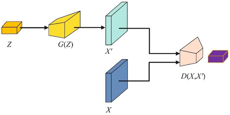
GAN model structure diagram.
The adversarial training of GAN is essentially a zero-sum game in game theory. The generator G takes random noise as input and processes it through neural networks to create realistic fake data that can deceive the discriminator D. Meanwhile, the discriminator strives to distinguish between real data and generated data. This adversarial relationship drives both networks to continuously improve through competition. In the GAN model, the generator G takes random noise Z as input and generates samples X′ with a distribution similar to the real samples X. The discriminator D receives both real samples X and generated samples X′ as input, aiming to distinguish between the generated data and the real data.
From the perspective of the discriminator, a stronger capability in this regard indicates superior discriminative efficacy. As such, the parameter optimization of the discriminator constitutes a process of maximizing the objective function, expressed as:
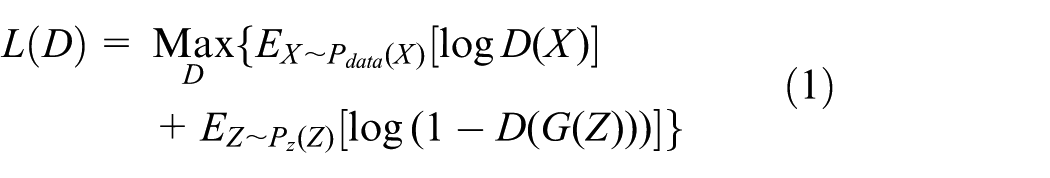
Here, X and Z, respectively, represent the real samples and random noise,
After the discriminator has been optimized, its parameters are fixed, and the optimization process proceeds to the generator. With the discriminator parameters held constant, the first term of the objective function, which relates to the discriminator, becomes a constant. Therefore, only the second term remains active during generator optimization. The training objective for the generator is to minimize this objective function, thereby encouraging the discriminator to classify generated samples as real. This process enhances the generator’s ability to deceive the discriminator. Thus, the optimization of the generator constitutes a process of minimizing the objective function, expressed as:

The optimization of GAN networks is a minimax process. First, the discriminator D is trained, and then the parameters of D are fixed to train the generator G. The objective function is as follows:
Through training, G and D engage in a two-player minimax game. The discriminator aims to maximize this objective function, whereas the generator seeks to minimize it. The ultimate optimization goal is to achieve a Nash equilibrium between the generator and discriminator, where the distribution of generated samples becomes virtually indistinguishable from that of real samples, indicating the generator has acquired strong generative capability. At this stage, the discriminator’s output probability for both real and generated data approaches 0.5, implying its inability to reliably distinguish the source of the input data.
Generalized generative adversarial network
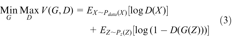
Existing anomaly detection methods have their own advantages and disadvantages: The AE structure is simple and training is efficient, but it is prone to overfitting normal data, resulting in insufficient anomaly detection ability; Ganomaly 24 improves the detection performance by learning the latent space distribution through GAN, but the training is unstable and prone to mode collapse; A dual-threshold attention-embedded GAN is proposed for generating high-quality infrared thermal (IRT) images to solve small-sample fault diagnosis of rotor-bearing system under time-varying speeds, 25 but the computational cost is high and the training is complex. Therefore, a GGAN is proposed, characterized by the following features: (1) It integrates the training stability of AE with the powerful data generation capability of GAN, thereby achieving accelerated model training; (2) by combining the reconstruction error from AE with the adversarial loss from discriminators, it attains high detection accuracy and enhanced robustness; (3) through dual encoders, contrastive learning, and multi-scale discrimination mechanisms, it enables effective anomaly detection under challenging conditions such as data imbalance and noise interference. Figure 2 illustrates the framework of the GGAN-based anomaly detection and its application workflow across different stages.
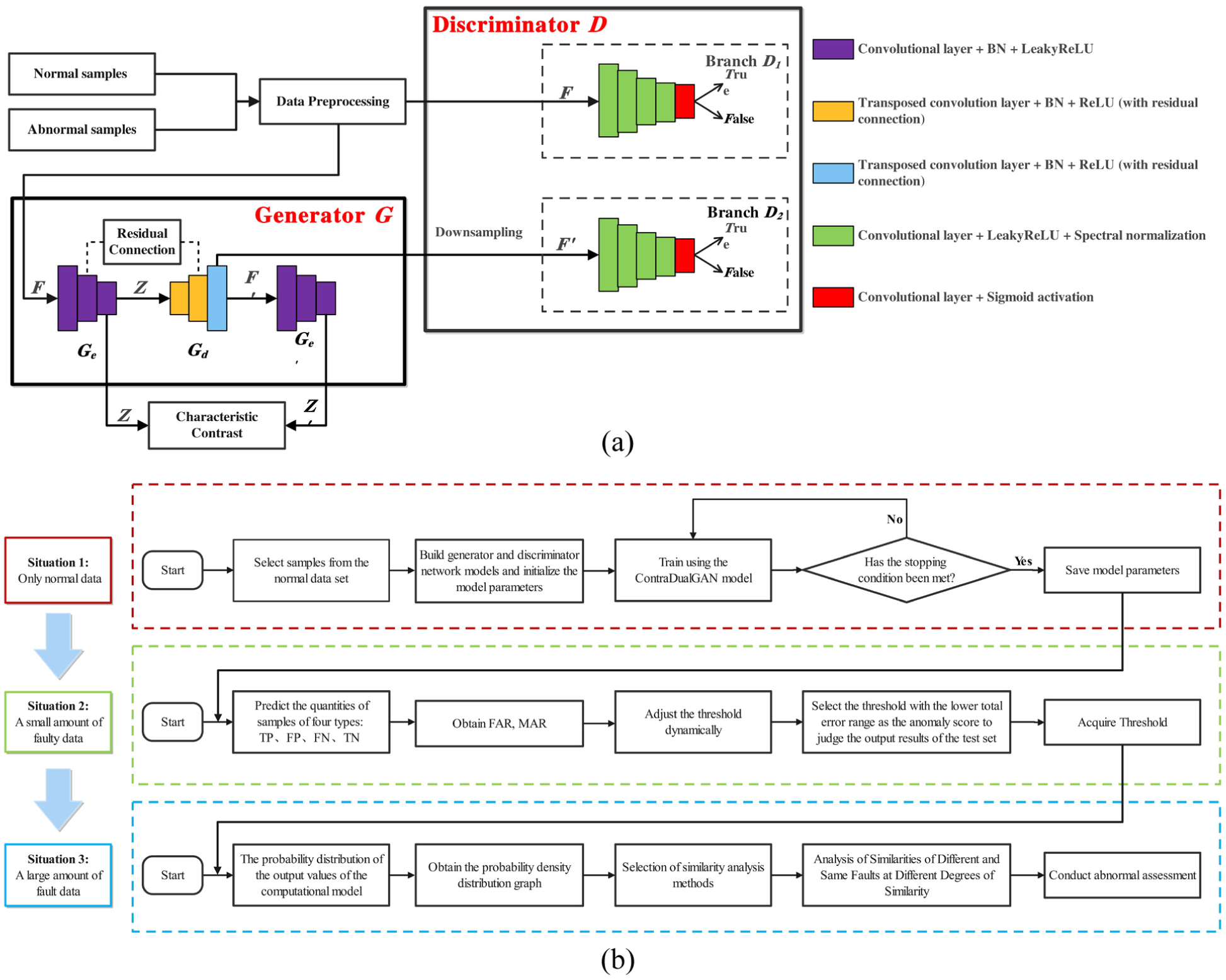
The framework of the GGAN-based anomaly detection (a) and its application workflow across different stages (b).
Figure 2(a) illustrates the framework of the anomaly detection model. The process begins with data preprocessing to obtain model samples. The generator then learns the data distribution of real samples and produces synthetic samples with similar characteristics. Meanwhile, the discriminator evaluates the authenticity of the output samples. Through adversarial training between the generator and discriminator, the model is continuously optimized until the distribution probability of the generated samples approximates that of the real samples.
Figure 2(b) demonstrates the application workflow of the model across different degradation stages. In the first stage, where the equipment operates normally without any fault data, the model is trained exclusively on normal data to learn the distribution of the normal data pattern. During the second stage, corresponding to the initial degradation phase with limited abnormal data, the model reduces errors by adjusting the decision threshold and evaluating outcomes. The third stage represents severe degradation, characterized by abundant fault data. By analyzing the anomaly scores and probability distributions of samples across different fault categories and severity levels, correlation coefficients are computed to enable fault identification and classification. Additionally, similarity features are leveraged to assess the degree of abnormality.
GGAN consists of generator G, discriminator D, contrastive learning and other components. The underlying principles of the model are described as follows:
Generator G
The Generator adopts a symmetric architecture of dual encoders and decoders, and achieves multi-scale feature fusion through residual connections.
Encoder G e
The input feature F is gradually reduced in dimension through three layers of convolution (kernel size = 8, stride = 2), and the output is the hidden layer feature Z. Each layer contains convolution, Batch Normalization, and LeakyReLU (α = 0.2) activation.

Decoder G d
The input is the hidden layer feature Z. Through three layers of transposed convolution (kernel size = 8, stride = 2), the feature F′ is reconstructed. The intermediate features corresponding to each stage of the encoder G e are fused in each layer (residual skip connections), and the activation functions are ReLU (in the intermediate layers) and Tanh (in the output layer).

Encoder G e ′
The structure is the same as that of G e but the parameters are independent. The input generates the feature F′, and the output is the hidden layer feature Z′.

Discriminator D
The discriminator adopts a multi-scale architecture and combines spectral normalization to enhance the training stability.
Branch D1
It processes the original input feature F, consisting of five layers of convolution (kernel size = 8 → 4, stride = 2), followed by spectral normalization and LeakyReLU (α = 0.2) activation, and outputs the discrimination probability.
Branch D2
It processes the downsampled generated feature F′, with parameters shared with D1, and outputs the discrimination probability.
Contrastive learning module
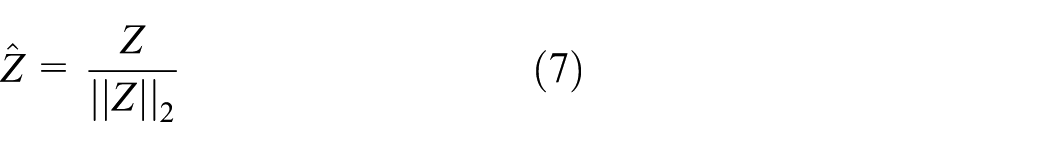
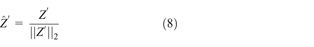
This module aims to enhance the model's consistency perception of normal patterns and sensitivity to abnormal signals through hidden layer feature alignment and maximizing distribution differences. Based on the noise-contrastive estimation (InfoNCE) 26 loss, combined with dynamic negative sample mining and memory library techniques, it optimizes the discriminability of features. The input features are the hidden layer features Z output by the encoder G e and Z′ output by the encoder G e ′, and they are L2 normalized to eliminate amplitude differences and focus on direction similarity.
Then, positive and negative sample pairs are constructed separately. Positive pairs consist of two samples from the same category or highly similar instances. In anomaly detection, positive pairs typically originate from different perspectives or augmented versions of the same normal sample. In this model, a positive pair refers to the hidden-layer features Z i extracted by encoder G e (from original normal input X i ) and features Z i ′ extracted by encoder G e ′ (from the generated reconstructed features of the same sample). The model aims to make Z i and Z i ′ as similar as possible in the feature space, enforcing tight coupling between the original and reconstructed features of normal samples in the latent space. Negative pairs consist of two samples from different categories or unrelated instances. In anomaly detection, negative pairs typically come from different normal samples or anomalous samples. In this model, a negative pair refers to features Z i extracted by G e (from normal sample X i ) and features Z j ′ extracted by G e ′ (from another normal sample X j where j ≠ i). The model aims to maximize dissimilarity between Z i and Z j ′ in feature space, thereby enhancing the learned boundaries between different samples. This mechanism helps better distinguish normal and anomalous instances. Overall, positive pairs serve to cluster features of similar samples, enhancing the model’s perception of normal patterns, while negative pairs push apart features of dissimilar samples to prevent confusion between normal and anomalous instances. This contrastive mechanism increases the model’s sensitivity to subtle faults, such as early gear wear. As a result, the model learns more discriminative features, which leads to a reduction in the false alarm rate.
The generator G learns the representations of the original input features F and the reconstructed features F′ through the use of two encoders G e and G e ′, and outputs the hidden layer features Z and Z′, respectively. It attempts to reconstruct the hidden layer features Z through the decoder G d and outputs the generated features F′. The discriminator uses a multi-scale discriminator to enhance its sensitivity to local anomalies (such as periodic transient impacts caused by gear cracks), and branches D1 input the original features F to determine whether F is real data; branch D2 inputs the generated features F′, and determines whether the low-resolution F′ is real data.
Loss function of the GAN model
The loss function of this model is mainly composed of two parts: generator loss L G and discriminator loss L D . It achieves the synergy of generative adversarial training and feature comparison learning through multi-objective optimization. The following details the definition, mathematical formulas, and other characteristics of each loss term in modules.
Generator loss (L G )
The generator loss integrates four parts: fraud loss, representation loss, latent loss, and contrast loss. The formula is:

Among them,
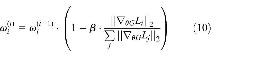
Here, β = 0.1 is the attenuation rate, aiming to prevent the single loss from dominating the optimization direction. The weight range is limited to
a. Adversarial loss (Lf)
The adversarial loss is mainly designed to induce the discriminator to misclassify the generated samples as real data, thereby pushing the generated distribution to approximate the real distribution. Its main function is to enhance the realism of the generated samples and avoid mode collapse. The specific formula is as follows:

Here, BCE refers to the binary cross entropy function; 1 represents the true label (0.9 is used for label smoothing processing), and the formula of binary cross entropy is as follows:
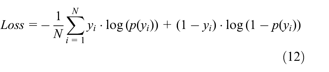
Here, y is either 1 or 0, and p(y) is the probability of outputting the label y.
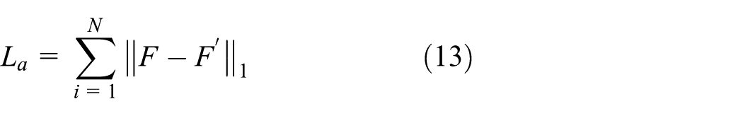
b. Characterizing loss (reconstruction loss, La)
The purpose of characterizing loss is to constrain the pixel-level similarity between the generated features and the original features. Compared with the L2 norm, the Manhattan distance (L1 norm) is more robust in detecting outliers and retains high-frequency details, thereby preventing the generator from over-optimizing the adversarial loss and ignoring local feature matching. The specific formula is as follows:
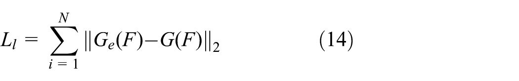
c. Latent loss (Ll)
The primary function of latent loss is to constrain the consistency of the hidden layer features output by Encoder G e and Encoder G e ′, aiming to force the alignment of the hidden layer feature representation Z′ of the generated feature F′ with the original feature Z, thereby enhancing the discriminative power of the latent space and suppressing the introduction of hidden layer offsets unrelated to the normal mode by the Generator. The specific formula is as follows:
d. Contrastive loss (Lc)
The contrastive loss is mainly based on the InfoNCE loss. It maximizes the similarity between positive samples and minimizes the similarity between negative samples, aligning the feature representations in the hidden layer space, amplifying the distribution shift of the hidden layer for abnormal samples, and enhancing the model’s sensitivity to subtle anomalies through the mining of difficult negative samples.
The definition of the contrastive loss function is as follows:
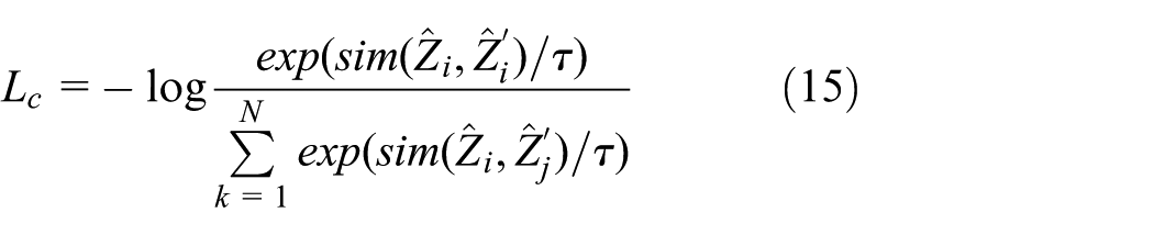
Among them, N is the batch size.
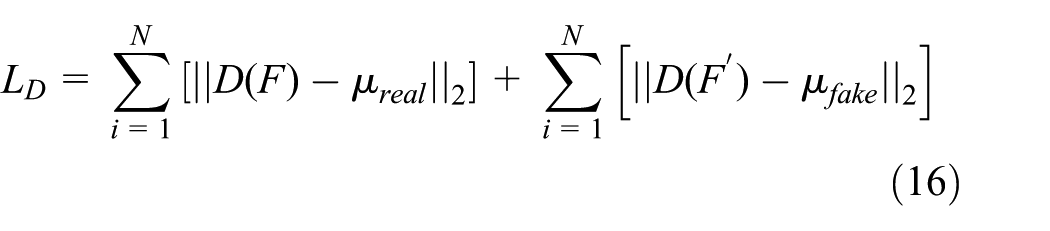
Discriminator loss (L D )
The discriminator loss adopts a feature matching strategy to avoid the instability caused by the binary classification loss in traditional GANs. It forces the discriminator to learn the distribution centers of real and generated data instead of the simple binary classification loss, alleviating the mode collapse problem, and improving the diversity of generation. The specific formula is as follows:
Herein,

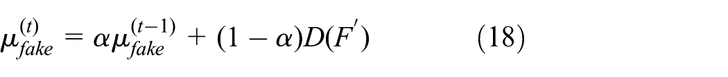
Among them, the sliding coefficient α is set to 0.9.
Experimental verification
Fault simulation experiment of a fixed-axle gearbox
Dataset introduction
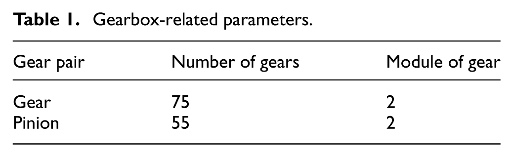
This dataset originates from the XJTUSpurgear test rig of the Aviation Engine Research Institute of Xi’an Jiaotong University 27 (the dataset is named: XJTUSpurgear dataset), as shown in Figure 3(a). The test rig consists of an electric motor, a gearbox, an axle, and a belt, etc. The electric motor is an AC variable frequency motor, and the vibration data is collected by the PCB333B32 accelerometer. In the experiment, a total of five vibration signals were collected, including four different degrees of gear crack faults and normal conditions. The four types of crack faults have depths of 0.2, 0.6, 1.0, and 1.4 mm, respectively, and the gear crack fault conditions are shown in Figure 3(b). This test simulated three rotational speed conditions, namely RPM900, RPM1200, and a variable rotational speed condition from 0 to RPM1200 and back to 0, with a sampling rate of 10 kHz. The relevant parameters of the gearbox are shown in Table 1.
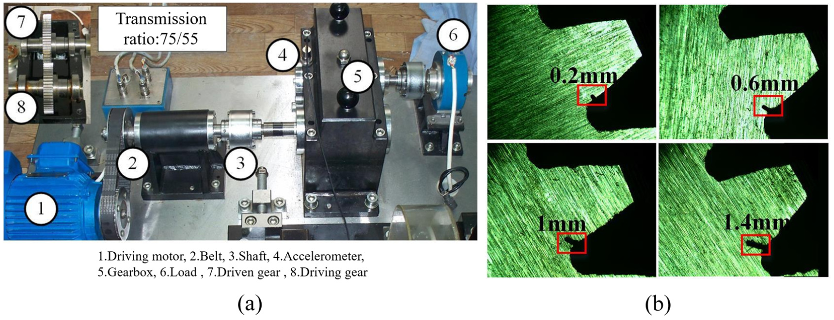
The test rig of XJTUSpurgear dataset: (a) the test rig and (b) health conditions of gear.
Gearbox-related parameters.
Abnormality detection evaluation
Anomaly detection was performed on datasets collected under two different speed conditions. The healthy condition was regarded as the normal class, whereas the remaining four crack-fault conditions were treated as anomalous samples. A subset of the dataset was used for model training. After training, the test set was fed into the trained anomaly detection model to obtain anomaly scores for individual samples. The samples were then classified as normal or abnormal according to the magnitude of the anomaly score. The dataset was split into training and testing sets at a ratio of 7:3.
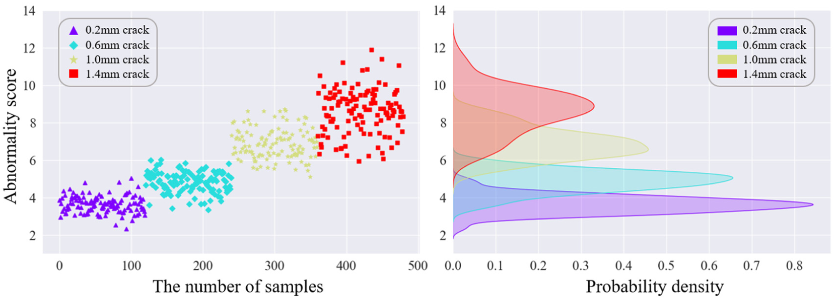
As shown in Figures 4 and 5, for the two speed conditions of RPM900 and RPM1200, the abnormality scores and probability density of the four crack faults of the test bench gears, are respectively shown. Different sample points represent different deep crack fault sample data: the purple triangle samples represent 0.2 mm fault samples; the blue rhombus samples represent 0.6 mm fault samples; the yellow pentagram samples represent 1.0 mm fault samples; the red square samples represent 1.4 mm fault samples. The left graph in the group chart is the result graph of abnormality scores for the four faults, with the vertical coordinate being the abnormality score of the sample and the horizontal coordinate being the number of samples corresponding to different samples, and the number of samples for each type of crack fault is 120; the right graph in the group chart is the probability density distribution graph of abnormality scores for the four faults, with the vertical coordinate being the abnormality score of the sample and the horizontal coordinate being the corresponding probability density.
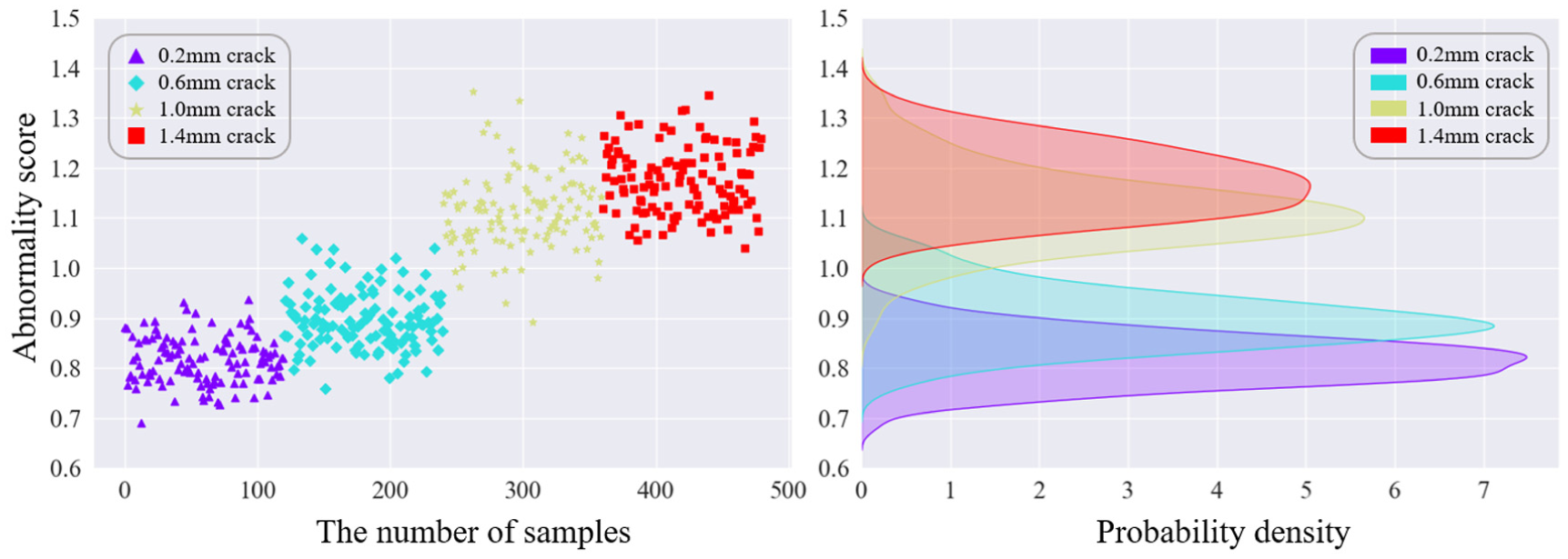
Anomaly scores and probability densities of cracked gear failures under RPM900.
Anomaly scores and probability densities of cracked gear failures under RPM1200.
Figure 4 depicts the anomaly score and probability density distribution of gear crack faults under the RPM900 operating condition. A clear positive correlation is observed, with the anomaly score increasing as the crack severity deepens. The anomaly score for the 0.2 mm crack is the lowest, ranging from 0.7 to 0.9, with the most concentrated distribution and the highest probability density (∼7.5) among the four fault levels. This indicates that the 0.2 mm crack represents an incipient fault, where the characteristics bear close resemblance to the normal state, making its detection particularly challenging. The 0.6 mm crack exhibits higher scores, yet its score range shows significant overlap with the 0.2 mm level, resulting in considerable misclassification and low discriminability. Compared to the 0.6 mm level, the 1.0 mm crack demonstrates a noticeable score increase and clearer separation, albeit with a more dispersed distribution. Finally, the 1.4 mm crack attains the highest scores, distributed between 1.1 and 1.3, but also demonstrates substantial overlap with the 1.0 mm level. This indicates a minor distinction between these two severe fault stages, where ambiguous anomalous features lead to identification errors.
Figure 5 depicts the anomaly scores and probability density distribution of gear crack faults under the RPM1200 condition. It can be observed that the anomaly score exhibits a gradual increase with the progression of crack severity. The 0.2 mm crack fault demonstrates the lowest anomaly scores, ranging from 3 to 4, with the most concentrated distribution and the highest probability density (∼0.85) among the four fault levels. However, when compared to the RPM900 condition, its probability density shows a significant discrepancy. Concurrently, all anomaly scores under this condition are universally higher than those at RPM900. The 0.6 mm crack fault exhibits higher scores than the 0.2 mm level, with only a minor overlap in their score ranges, indicating a certain degree of error. The 1.0 mm crack fault shows a further score increase and a more distinct separation from the 0.6 mm level, though its distribution is relatively dispersed compared to other faults. The 1.4 mm crack fault registers the highest scores, which are also the most scattered, distributed across a wide range of 6–12. As illustrated in Figure 5, the model achieves effective discrimination between different crack fault levels under the RPM1200 condition, demonstrating satisfactory performance.
Overall, under different operating conditions, the anomaly scores demonstrate a discernible differentiation across various fault severities, and exhibit a positive correlation with the progression of the crack fault. Under the RPM900 condition, a pronounced distinction exists between the anomaly scores of the minor faults (0.2 and 0.6 mm cracks) and the severe faults (1.0 and 1.4 mm cracks). However, a certain degree of misclassification is observed due to overlapping score ranges within the two minor fault levels and within the two severe fault levels. In contrast, under the RPM1200 condition, the anomaly score ranges for different fault types are distinct and well-separated, resulting in a more significant and effective detection performance. The accuracy of this anomaly detection model under both operational conditions is summarized in Table 2.
XJTUSpurgear dataset anomaly detection accuracy.
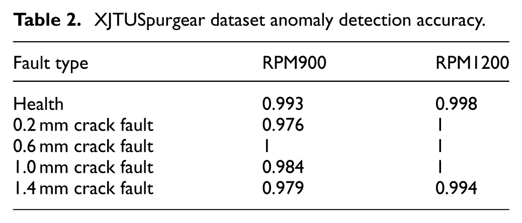
As can be seen from Table 2, the abnormal detection accuracy rates of most crack fault degrees are relatively high. Almost all faults can be detected, and the accuracy rate of some faults can even reach 100%. Since the crack fault feature of 0.2 mm on the gear is quite similar to the feature of normal samples, some samples under the RPM900 operating condition and RPM1200 operating condition are identified as normal. Particularly under the RPM900 operating condition, a small part of the samples with 0.2 mm crack faults are identified as healthy and fault-free. Overall, the abnormal detection accuracy rate has reached over 97%.
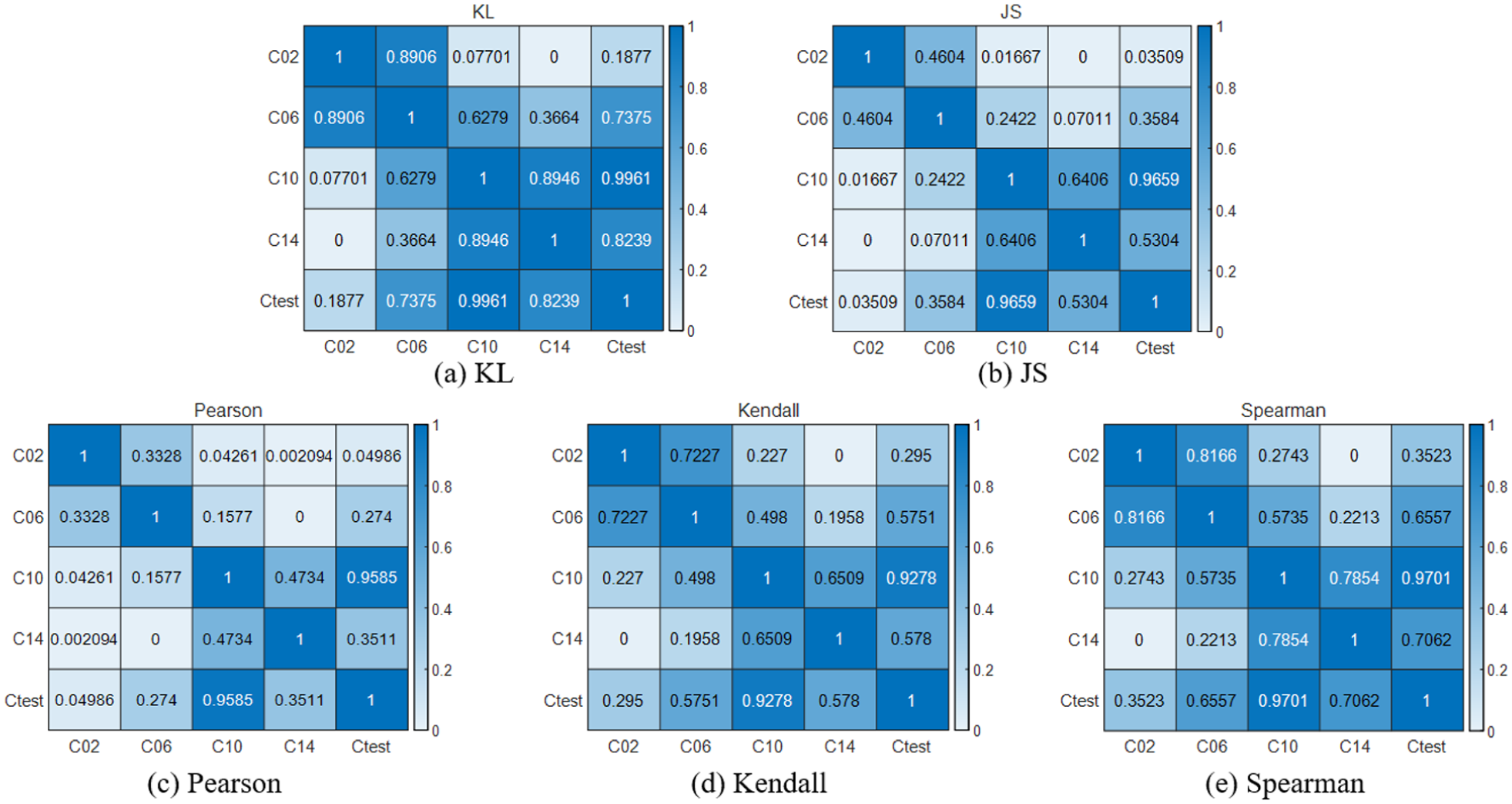
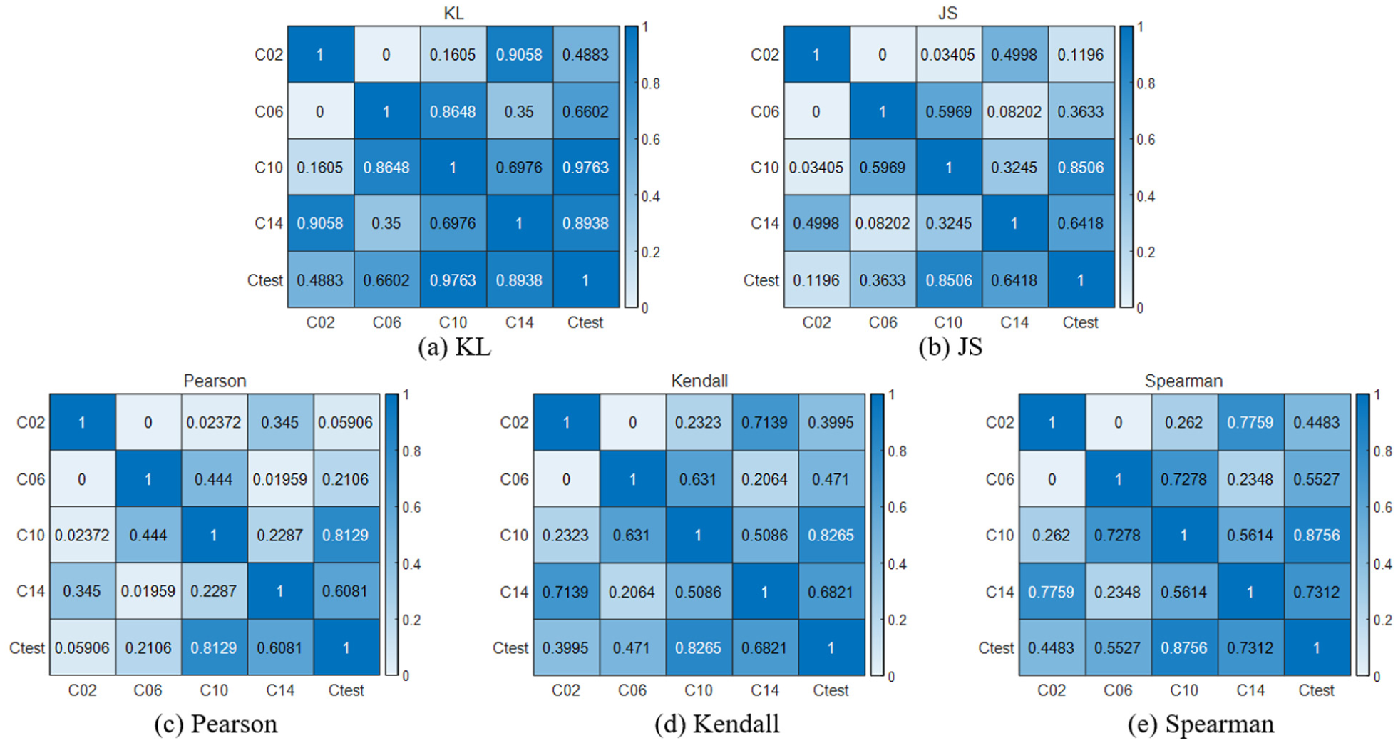
This paper adopts five similarity analysis methods, namely KL distance, JS distance, Pearson correlation coefficient, Kendall correlation coefficient, and Spearman correlation coefficient, to compare and analyze the similarities between the distribution patterns of different degrees of crack faults observed under different operating conditions. This helps to determine the similarity degree between new faults and existing fault categories. It can also calculate the accuracy of fault classification and facilitate fault identification. Firstly, the five correlation analysis methods are used to analyze the four crack faults under the RPM900 operating condition and RPM1200 operating condition, respectively. The results are shown in Figures 6 and 7.
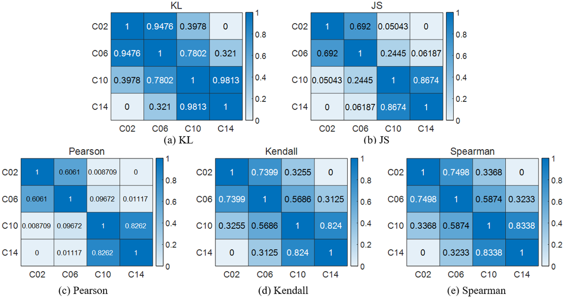
Results of correlation analysis of four crack failures in gears under RPM900: (a) KL, (b) JS, (c) Pearson, (d) Kendall, and (e) Spearman.
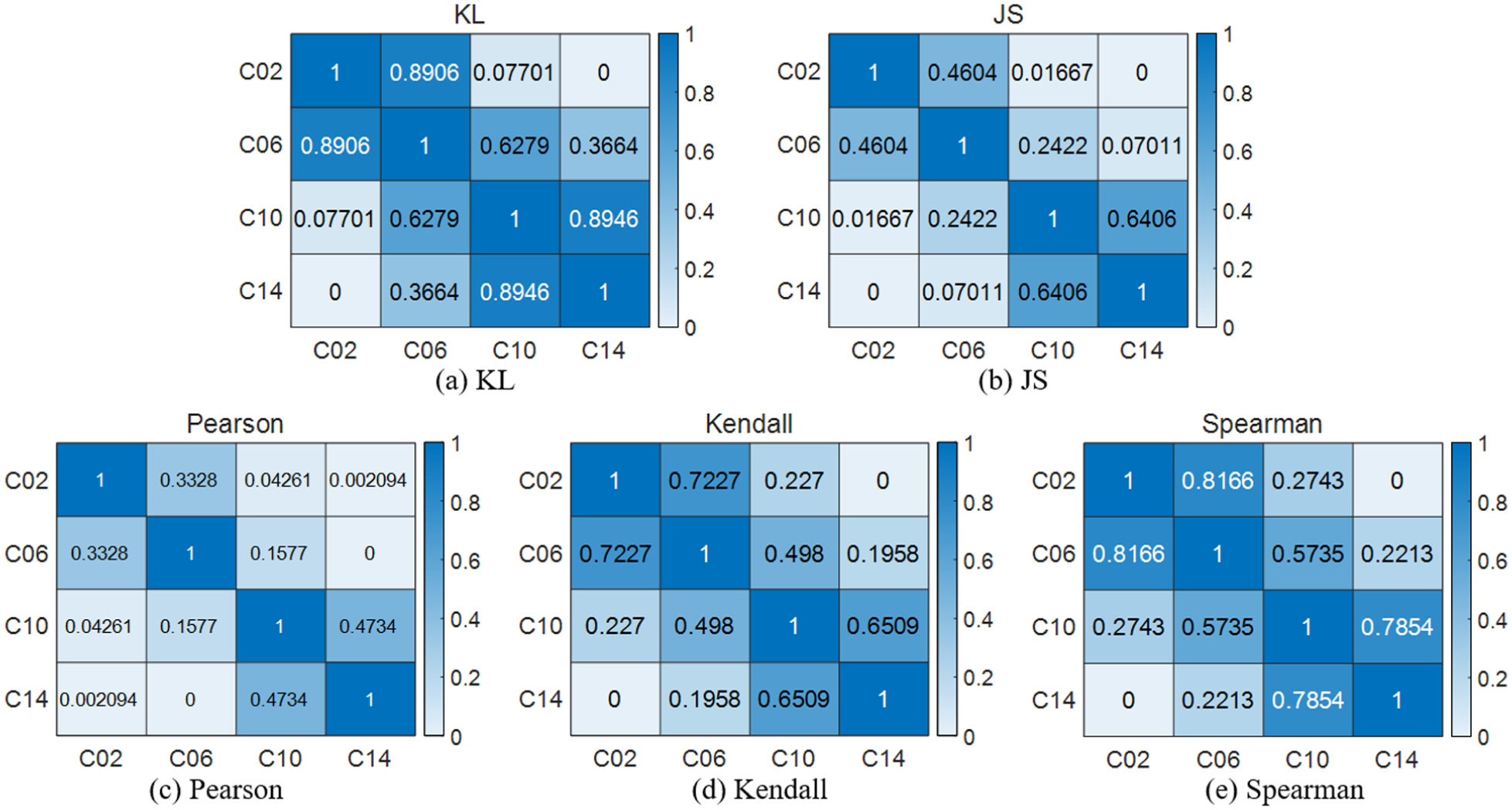
Results of correlation analysis of four crack failures in gears under RPM1200: (a) KL, (b) JS, (c) Pearson, (d) Kendall, and (e) Spearman.
In Figure 6, C02, C06, C10, and C14 represent four different crack failure degrees under RPM900 working condition, namely 0.2 mm depth crack failure, 0.6 mm depth crack failure, 1.0 mm depth crack failure, and 1.4 mm depth crack failure. From Figure 6(c), it can be seen that the similarity degrees of the fault types similar to C06 are 0.6061, 0.09672, and 0.01117, respectively, among which the largest one is 0.6061. Compared with other similarity analysis methods, the largest similarity degrees are 0.9476, 0.692, 0.7399, and 0.7498, respectively. Since the correlation is smaller, the fault type discrimination is better, so the Pearson distance similarity analysis method has the best analysis effect under RPM900 working condition and the similarity scores between different faults are also the smallest. From Figure 6(a), it can be seen that the similarity degrees of the fault types similar to C10 are 0.3978, 0.7802, and 0.9813, respectively, among which the largest one is 0.9813. Compared with other similarity analysis methods, the largest similarity degrees are 0.8674, 0.8262, 0.824, and 0.8338, respectively. Since the correlation is larger, the fault type discrimination is worse, so the KL correlation coefficient analysis method has the worst effect under RPM900 working condition.
As can be seen from Figure 7(c), the maximum similarity to the C10 fault type is 0.4734. Therefore, under the RPM1200 condition, the Pearson-distance-based similarity analysis performs best, and the similarity scores among different faults are also the lowest. In contrast, Figure 7(a) shows that the maximum similarity to the C06 fault type reaches 0.8906. Therefore, under RPM1200 condition, the KL correlation-coefficient-based method yields the poorest performance.
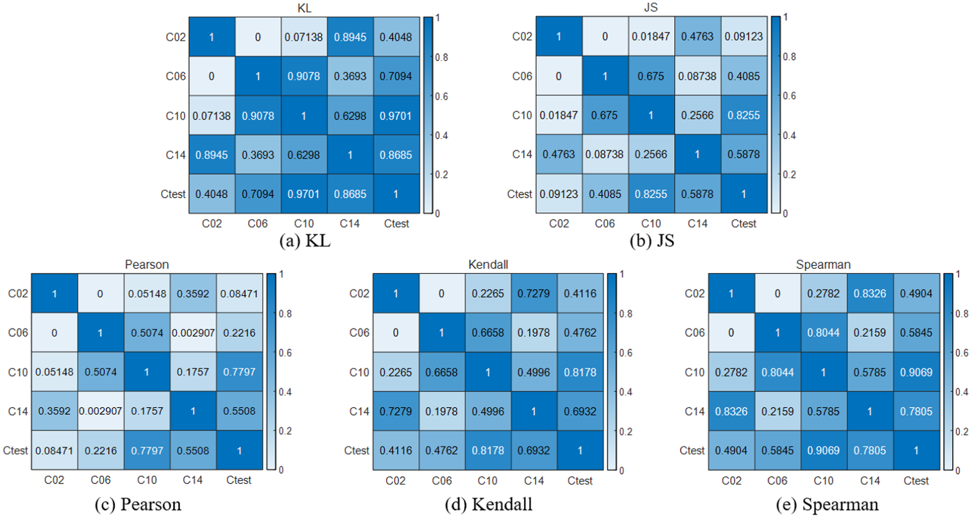
Under the operating condition of RPM1200, the test data “Ctest” with unknown crack failure degree is selected, and the GGAN model is used for analysis. Firstly, the abnormal score is calculated, then the probability density graph of the abnormal score is generated, as shown in Figure 8. The probability density graph of the abnormal score and the test data is displayed in the figure. Subsequently, the similarity analysis between the test data and the known data is conducted, and the analysis results are normalized. Figure 9 shows the similarity analysis results normalized by using the GGAN model.

Test data Ctest anomaly score and probability density.
Correlation analysis results based on the GGAN model: (a) KL, (b) JS, (c) Pearson, (d) Kendall, and (e) Spearman.
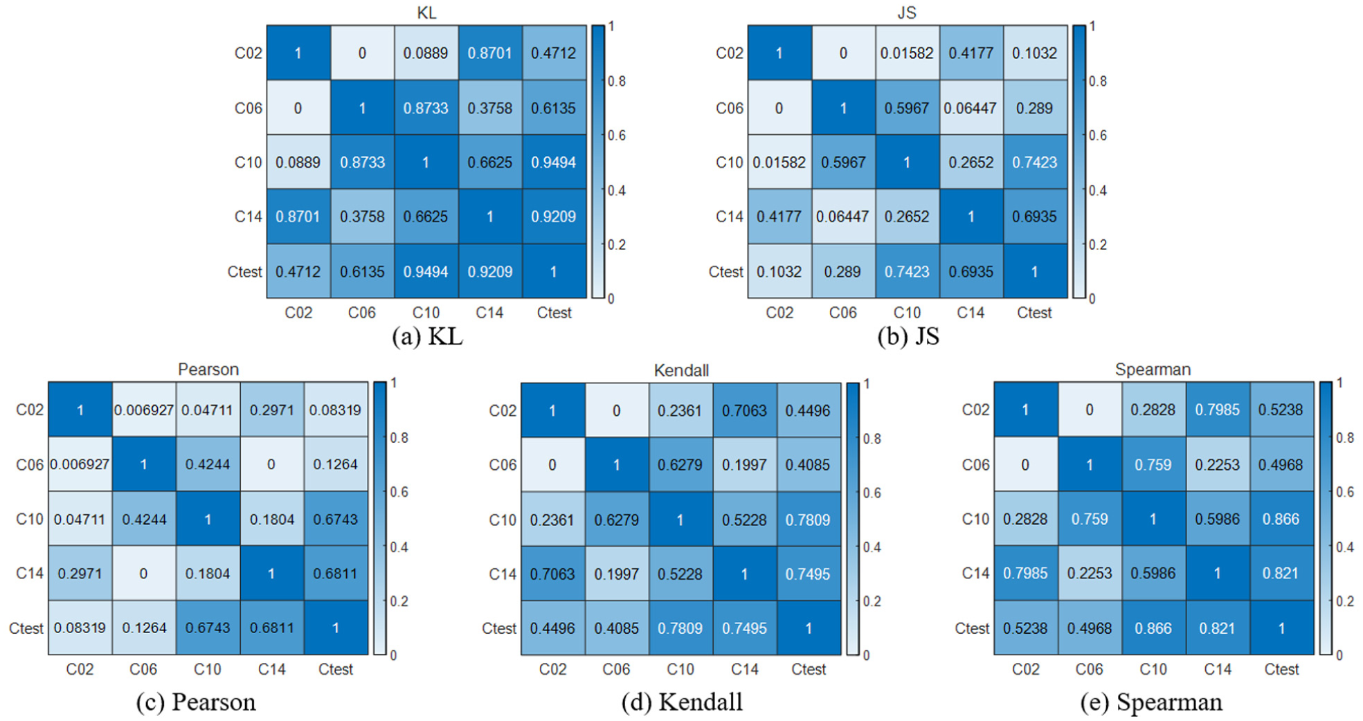
During the evaluation stage, the normalized similarity index between the test data and the known data is fused to assess the fault condition, that is, most similar to the test data. The GGAN model is replaced with IGAN, GANomaly, and AE, and anomaly detection is conducted under the same operating conditions. The same test data is selected for comparative analysis to obtain the comprehensive similarity assessment results of different models, as shown in Figures 10 to 12. The comprehensive similarity assessment results of different models are presented in Table 3 and Figure 13.
Correlation analysis results based on the IGAN model: (a) KL, (b) JS, (c) Pearson, (d) Kendall, and (e) Spearman.
Correlation analysis results based on the GANomaly model: (a) KL, (b) JS, (c) Pearson, (d) Kendall, and (e) Spearman.
Correlation analysis results based on the AE model: (a) KL, (b) JS, (c) Pearson, (d) Kendall, and (e) Spearman.
Combined anomaly assessment results from different models.
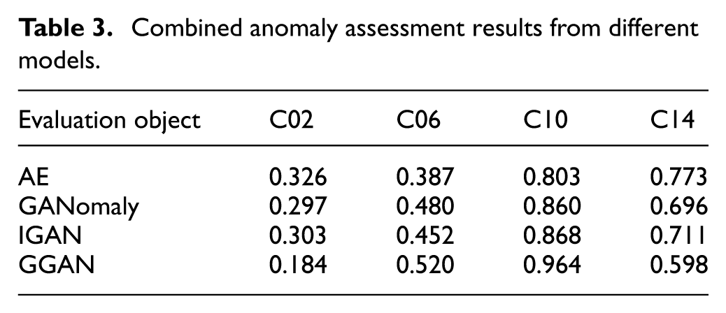
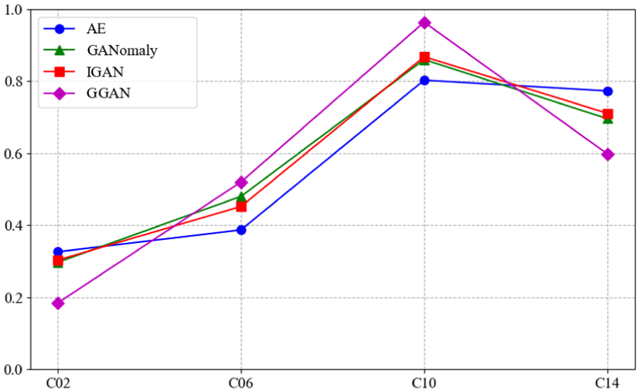
Combined anomaly assessment results from different models.
From Table 3 and Figure 13, it can be seen that among the results of the four models, the comprehensive abnormal assessment result score, that is, the highest for all is C10. This indicates that the crack fault degree characteristics of the test data are most similar to C10. Based on this result analysis, it can be concluded that the crack fault degree of the test data corresponds to C10, that is, a 1.0 mm deep crack fault. The results show that this framework can accurately assess the fault degree of the test data.
Fault simulation experiment of a planetary gearbox
Dataset introduction
Test rig description
To facilitate the related research, a planetary gearbox fault simulation test rig, as shown in Figure 14, was designed and constructed in this study. The test rig mainly consists of six components: a driving motor, a torque–speed sensor, a planetary gearbox, an encoder, a radial loading device, and an intelligent loading system.
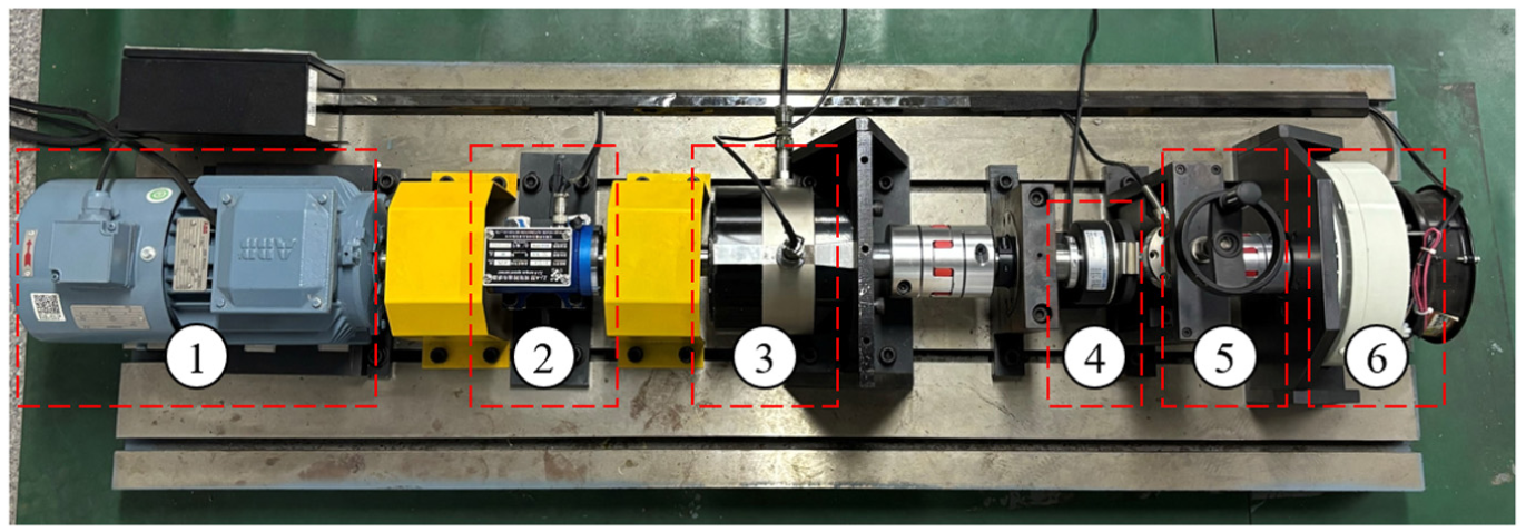
Planetary gearbox fault simulation test rig: (1) drive motor, (2) torque-speed sensor, (3) planetary gearbox, (4) encoder, (5) radial loader, and (6) intelligent loading device.
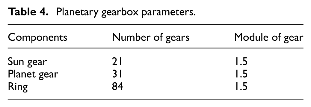
The driving motor is a 1.1 kW variable-frequency motor equipped with protection functions against overcurrent, overvoltage, overload, overheating, and undervoltage. With the aid of a motor support adjustment system, the motor allows adjustment of horizontal eccentricity within ±3 mm, angular misalignment within ±2.5°, and parallel misalignment up to +1 mm. Serving as the power source of the test rig, the motor has a rated voltage of 380 V and a rated speed of 1000 r/min. The torque–speed sensor is primarily used to monitor the torque variation on the rotating shaft in real time, analyze the load conditions of the transmission system, and ensure that the equipment operates within a safe range. In addition, it measures the rotational speed of the shaft, from which the output power can be calculated. The planetary gearbox is employed to simulate the planetary gear transmission system of a wind turbine gearbox and consists of one sun gear and three planet gears. The detailed parameters of the planetary gearbox are listed in Table 4.
Planetary gearbox parameters.
Test components description
In this experiment, sun gears with different severities of tooth breakage were employed to simulate faults in the planetary gearbox. The fault severities of the sun gear include 25% tooth breakage, 50% tooth breakage, and 75% tooth breakage. The fault simulation components are shown in Figure 15.
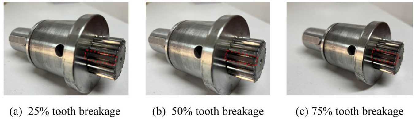
Simulation of sun gear tooth breakage fault: (a) 25% tooth breakage, (b) 50% tooth breakage, and (c) 75% tooth breakage.
Signal acquisition and experimental procedure
This study is based on a planetary gearbox fault-simulation test rig. Experiments were carried out under four component conditions: a healthy state and three levels of sun gear tooth breakage severity. The baseline operating parameters were set to a sampling frequency of 51.2 kHz and a recording duration of 600 s. The drive motor was operated at a nominal speed of 300 r/min. After the drivetrain reached steady-state operation, baseline data were collected under no-load conditions. Each test was repeated twice to eliminate random errors.
The load and motor speed settings for the four test conditions are summarized in Table 5. After replacing the gear component or adjusting the operating parameters, the drivetrain was allowed to run until transient responses fully decayed (typically 3–5 min). Formal data acquisition was initiated once the vibration signals became stable, ensuring consistent operating conditions across all tests.
Test conditions of planetary gearbox fault-simulation.
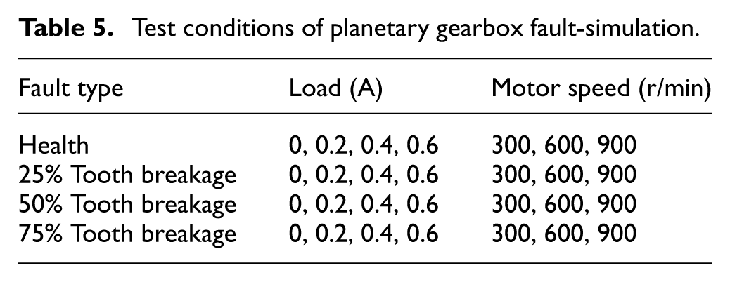
To validate the effectiveness of the proposed framework, vibration datasets from four health states were used for anomaly evaluation under three operating conditions (load = 0.2 A; motor speed = 300, 600, and 900 r/min). A similarity-analysis-based method was then employed to assess anomalies. The detailed evaluation results are presented in the following section.
Abnormality detection evaluation
Similar to the anomaly detection procedure for the fixed-axis gearbox, anomaly detection was conducted on datasets from the planetary gearbox under three different speed conditions. The healthy condition was treated as the normal class, whereas the other three tooth-breakage fault conditions were treated as anomalies. The dataset was split into training and testing sets at a ratio of 7:3.
Anomaly evaluation was performed for the sun gear fault conditions. Figures 16 to 18 present the anomaly scores and probability density distributions of three sun gear tooth-breakage severities under three speed conditions. Each marker corresponds to a sample from a specific fault class: purple triangles denote the 25% tooth-breakage fault, green diamonds denote the 50% tooth-breakage fault, and red pentagrams denote the 75% tooth-breakage fault. In each figure, the left panel shows the anomaly-score results for the three fault severities, where the y-axis represents the anomaly score and the x-axis indicates the sample index; each class contains 120 samples. The right panel shows the probability density distributions of the anomaly scores for the three faults, with the y-axis representing the anomaly score and the x-axis representing the corresponding probability density.
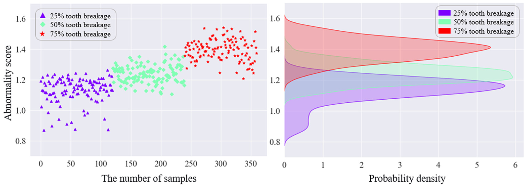
Anomaly scores and probability densities of sun gear under RPM300.
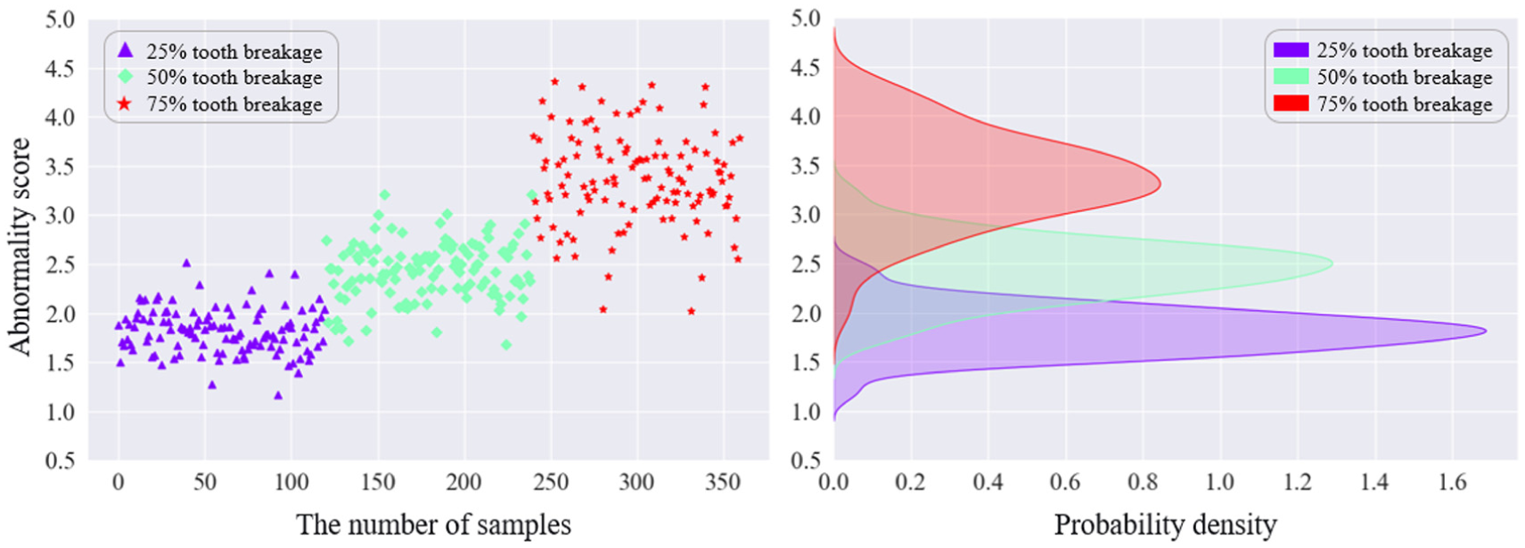
Anomaly scores and probability densities of sun gear under RPM600.
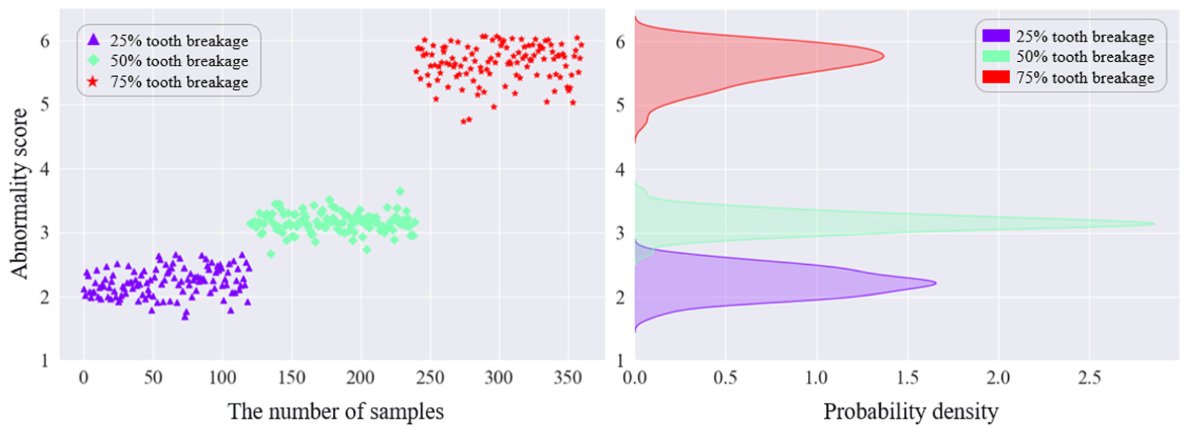
Anomaly scores and probability densities of sun gear under RPM900.
Overall, under different operating conditions, the anomaly scores show a certain degree of separability among different tooth-breakage severities, and the anomaly score increases as the fault severity deepens. Under the RPM300 condition, the anomaly-score ranges of different severities overlap, leading to relatively large errors. Under RPM600, samples with different tooth-breakage severities can be effectively distinguished, although some errors still exist. Under RPM900, the anomaly-score ranges of different severities do not overlap and the separation is much clearer, indicating more pronounced detection performance. The accuracy of the anomaly detection model under the three operating conditions is listed in Table 6.
Accuracy of anomaly detection in test rig datasets.
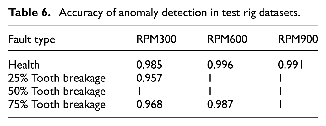
As shown in Table 6, the anomaly detection accuracy is high for most tooth-breakage, and the vast majority of faults can be successfully detected; for some fault cases, the accuracy reaches 100%. Under the RPM300 condition, some samples of the 25% sun gear tooth-breakage fault exhibit anomaly-score characteristics close to those of healthy samples, and a portion of 75% sun gear tooth-breakage samples are assessed as 50% severity, which leads to false alarms/misclassifications. Under RPM600, a small number of 75% sun gear tooth-breakage samples are also identified as other severity levels. Overall, the anomaly detection accuracy exceeds 95%.
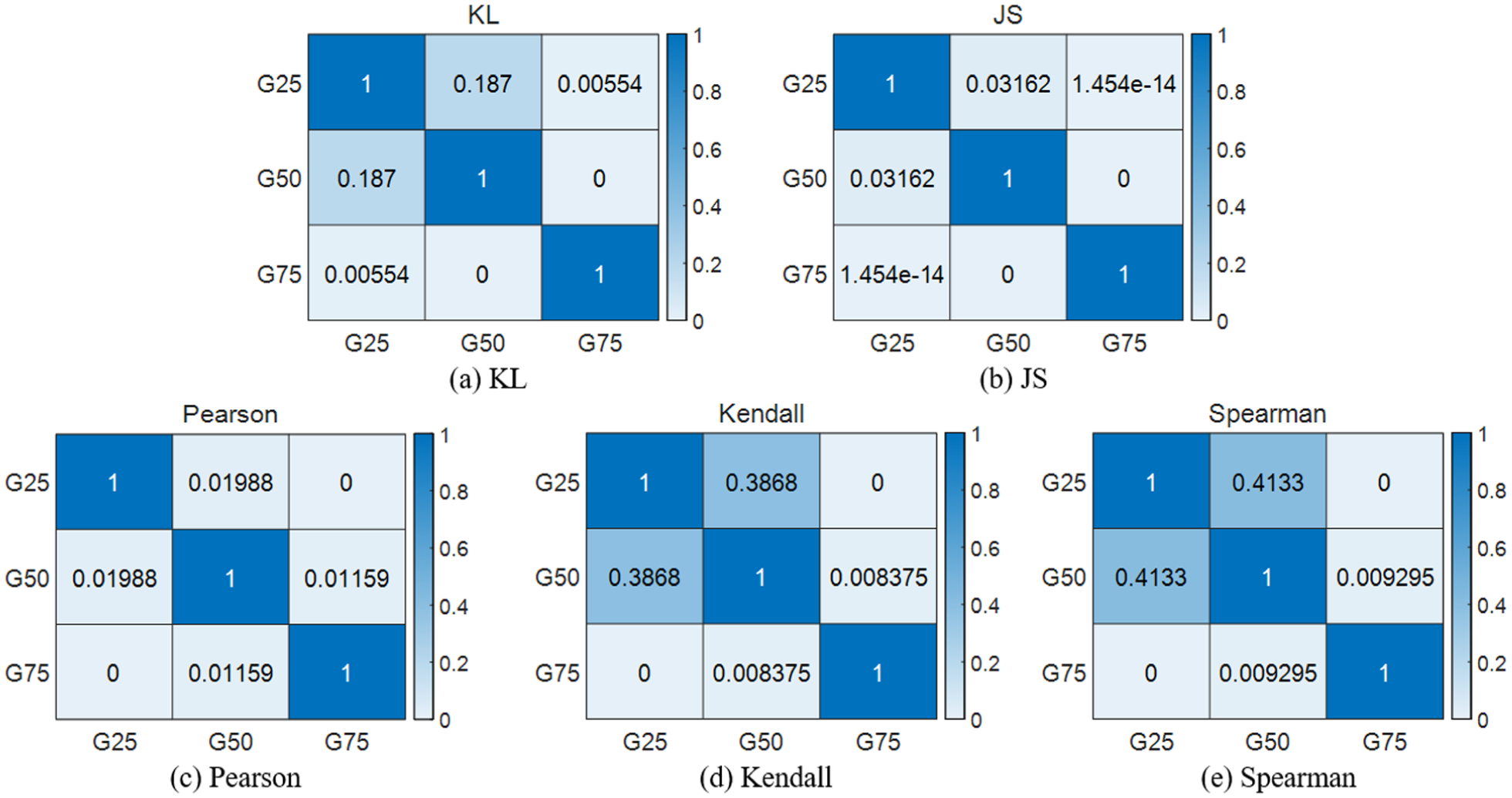
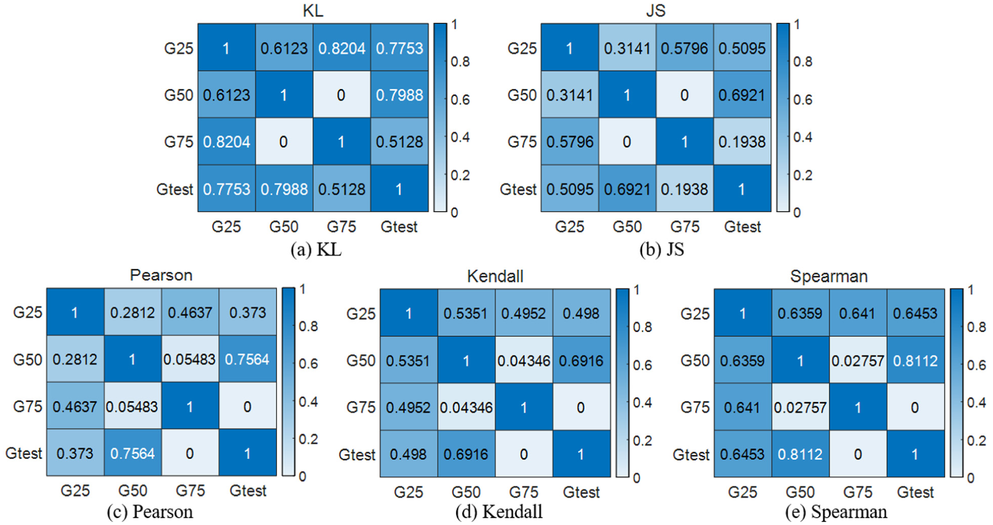
Five similarity-analysis methods were employed to comparatively evaluate the similarity among different tooth-breakage severities under various operating conditions, which helps quantify how closely a newly observed fault resembles the predefined severity levels. In addition, these methods can be used to compute the accuracy of fault classification, thereby facilitating fault identification. The three fault severities were analyzed separately under RPM300, RPM600, and RPM900, and the results are presented in Figures 19 to 21. In each figure, subplots (a) to (e) correspond to the KL distance, JS distance, Pearson correlation coefficient, Kendall’s tau correlation coefficient, and Spearman correlation coefficient, respectively.
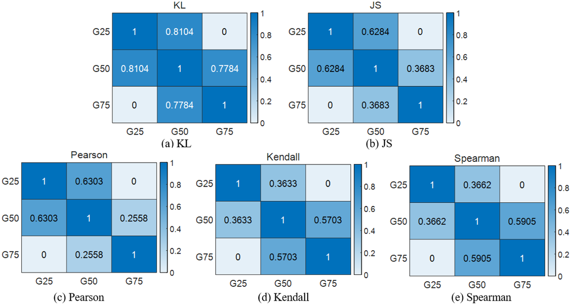
Results of correlation analysis of different tooth-breakage severities under RPM300: (a) KL, (b) JS, (c) Pearson, (d) Kendall, and (e) Spearman.
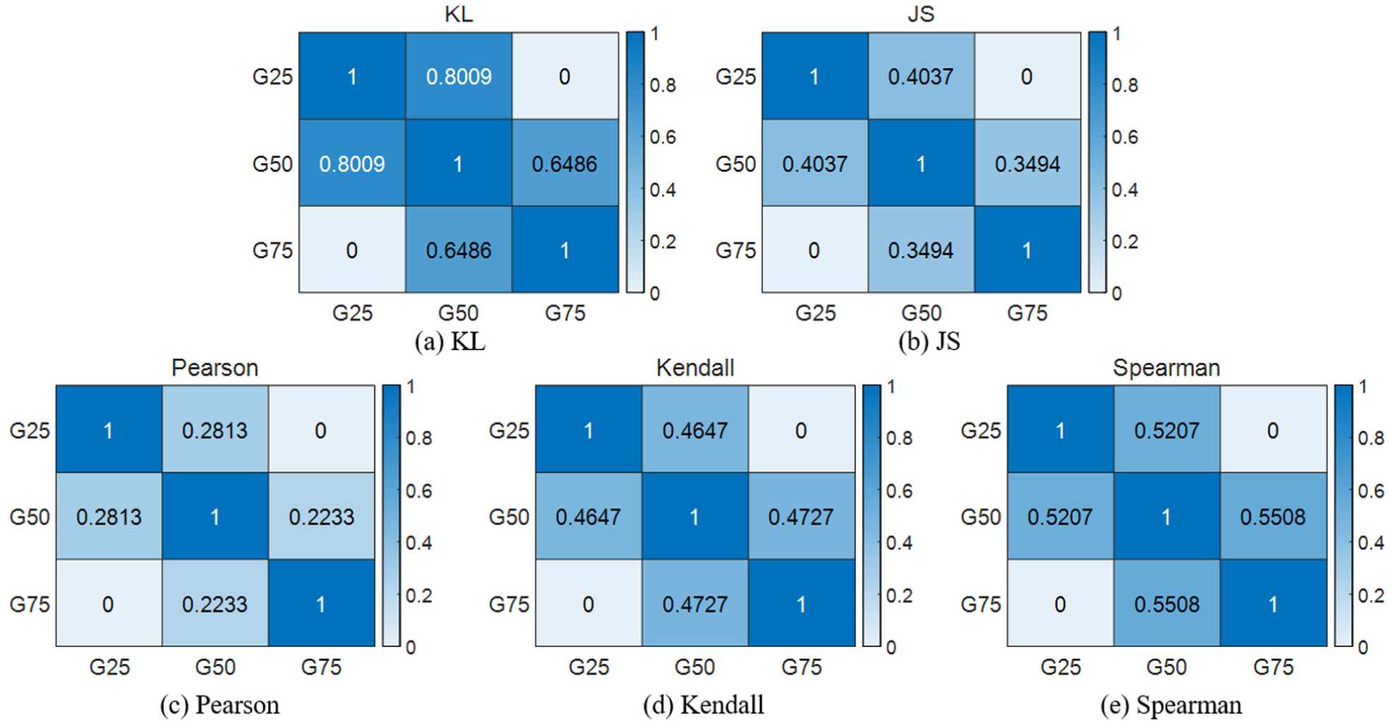
Results of correlation analysis of different tooth-breakage severities under RPM600: (a) KL, (b) JS, (c) Pearson, (d) Kendall, and (e) Spearman.
Results of correlation analysis of different tooth-breakage severities under RPM900: (a) KL, (b) JS, (c) Pearson, (d) Kendall, and (e) Spearman.
In Figure 19, G25, G50, and G75 denote the sun gear tooth-breakage faults with 25%, 50%, and 75% damage severity, respectively, under the RPM300 condition. As shown in Figure 19(d), the similarity between G25 and G50 reaches 0.3633. By comparison, the corresponding similarities given by the other methods are 0.8104, 0.6284, 0.6303, and 0.3622. Since a lower correlation indicates better separability between fault severities, the Kendall-based similarity analysis provides the best performance, yielding the smallest similarity scores between different faults. In contrast, Figure 19(a) shows that G75 is most similar to G50, with a similarity of 0.7784; the similarities obtained by the other methods are 0.3683, 0.2558, 0.5703, and 0.5905, respectively. Because higher correlation implies poorer distinguishability among fault types, the KL-based method exhibits the worst performance.
As shown in Figure 20(c), the similarity between G25 and G50 is 0.2813. In comparison, the similarities obtained by the other methods are 0.8009, 0.4037, 0.4647, and 0.5207, respectively. Therefore, the Pearson-based similarity analysis performs best, yielding the smallest similarity scores between different faults. In contrast, Figure 20(a) shows that the similarity between G50 and G75 is 0.6486, which is the largest among the evaluated methods, implying poorer separability between fault types; hence, the KL-based method exhibits the worst performance.
As shown in Figure 21(c), the similarity between G25 and G50 is 0.01988, which is the smallest among the analyzed methods. Since smaller similarity indicates better discrimination, the Pearson-based similarity analysis provides the best performance, with the lowest similarity scores between different fault severities. Meanwhile, Figure 21(e) shows that the maximum similarity among different severities is 0.4133. The Spearman-based similarity analysis yields the highest overall similarity score, indicating the poorest performance and making it more difficult to distinguish different fault types.
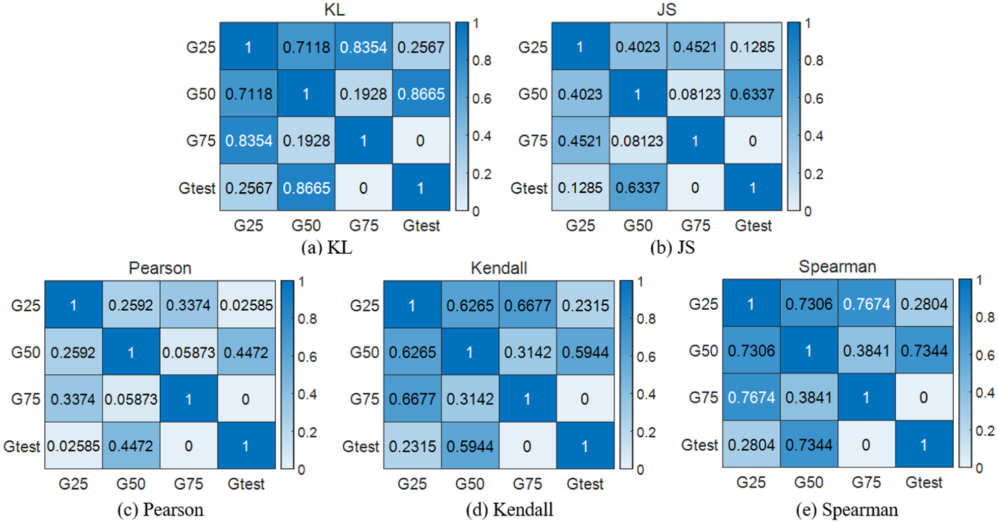
To evaluate data with an unknown fault severity, a test dataset denoted as “Gtest” was selected under the RPM600 condition and analyzed using the GGAN model. First, anomaly scores were computed and the probability density distribution of the anomaly scores was plotted, as shown in Figure 22, which presents the anomaly scores and the probability density of the test data. Subsequently, similarity analysis was performed between the test data and the known datasets, and the similarity scores were normalized. Figure 23 shows the normalized similarity-analysis results obtained using the GGAN model.
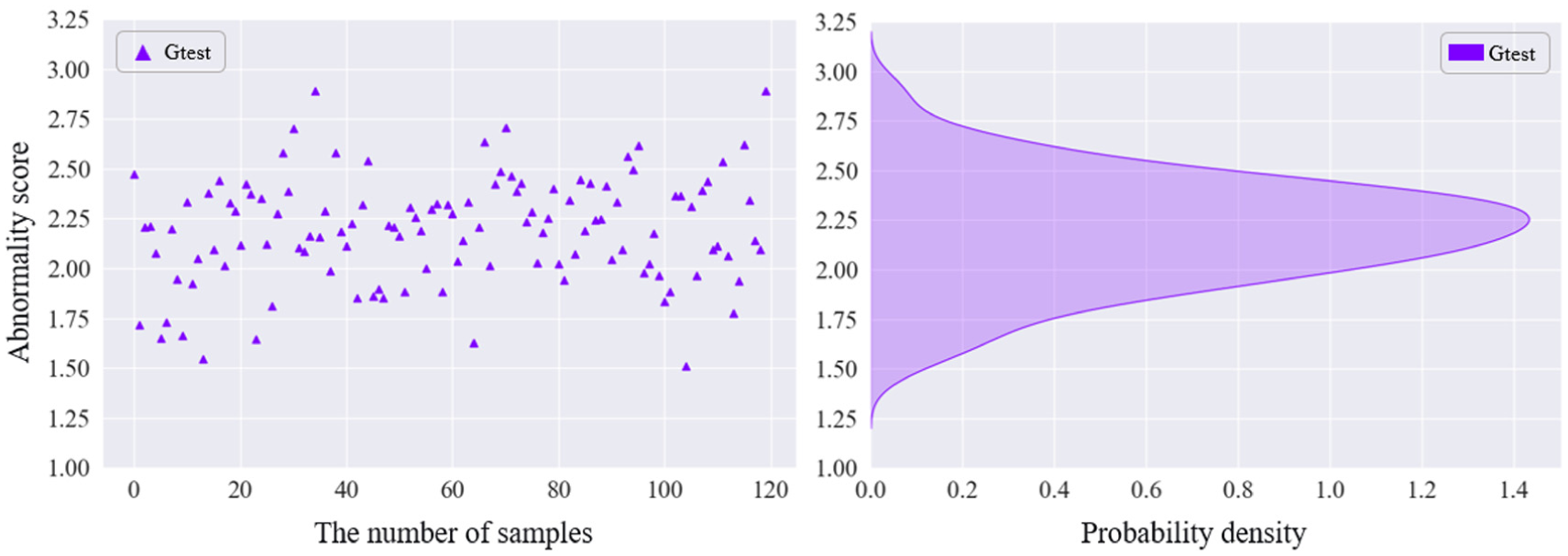
Test data Gtest anomaly score and probability density.
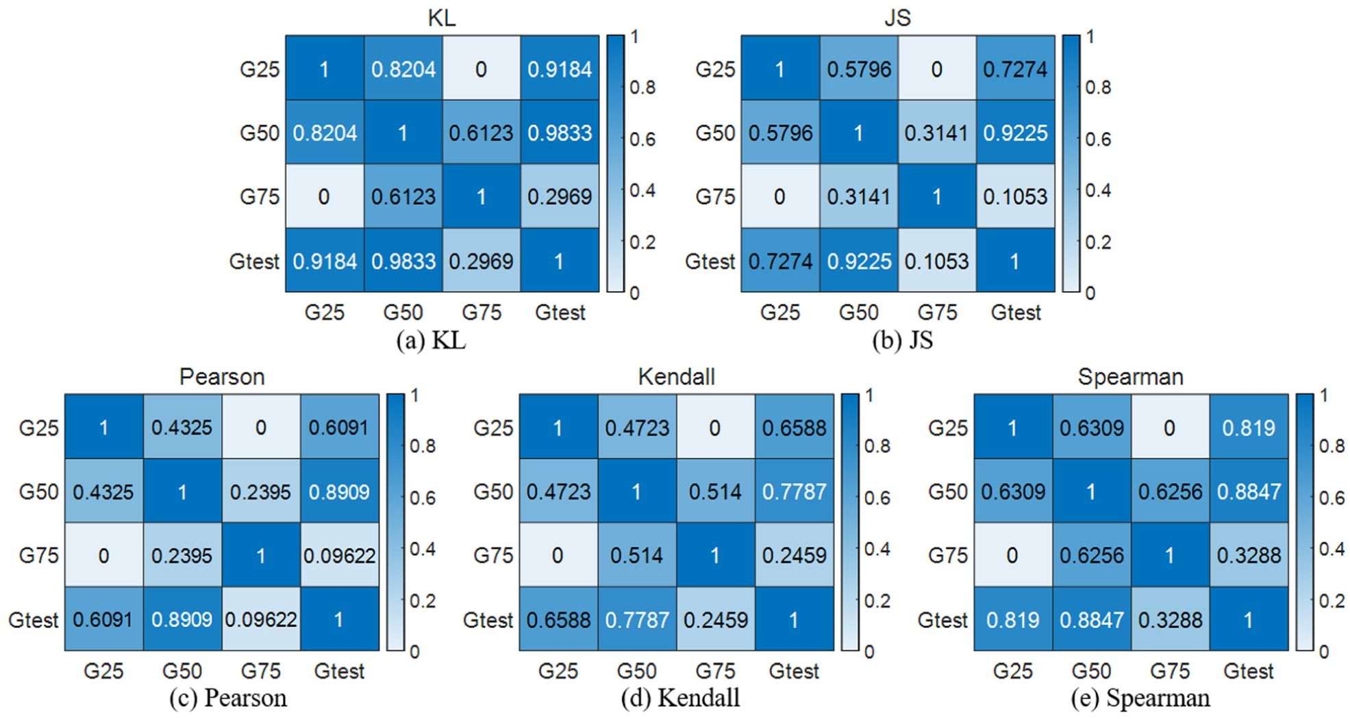
Correlation analysis results based on the GGAN model: (a) KL, (b) JS, (c) Pearson, (d) Kendall, and (e) Spearman.
During the evaluation stage, the normalized similarity indices between the test data and the known datasets were fused to identify the fault condition most similar to the test data. The GGAN model was then replaced with IGAN, GANomaly, and AE, and anomaly detection was performed under the same operating condition. Using the same test dataset for comparative analysis, the integrated anomaly evaluation results of the different models were obtained, as shown in Figures 24 to 26.
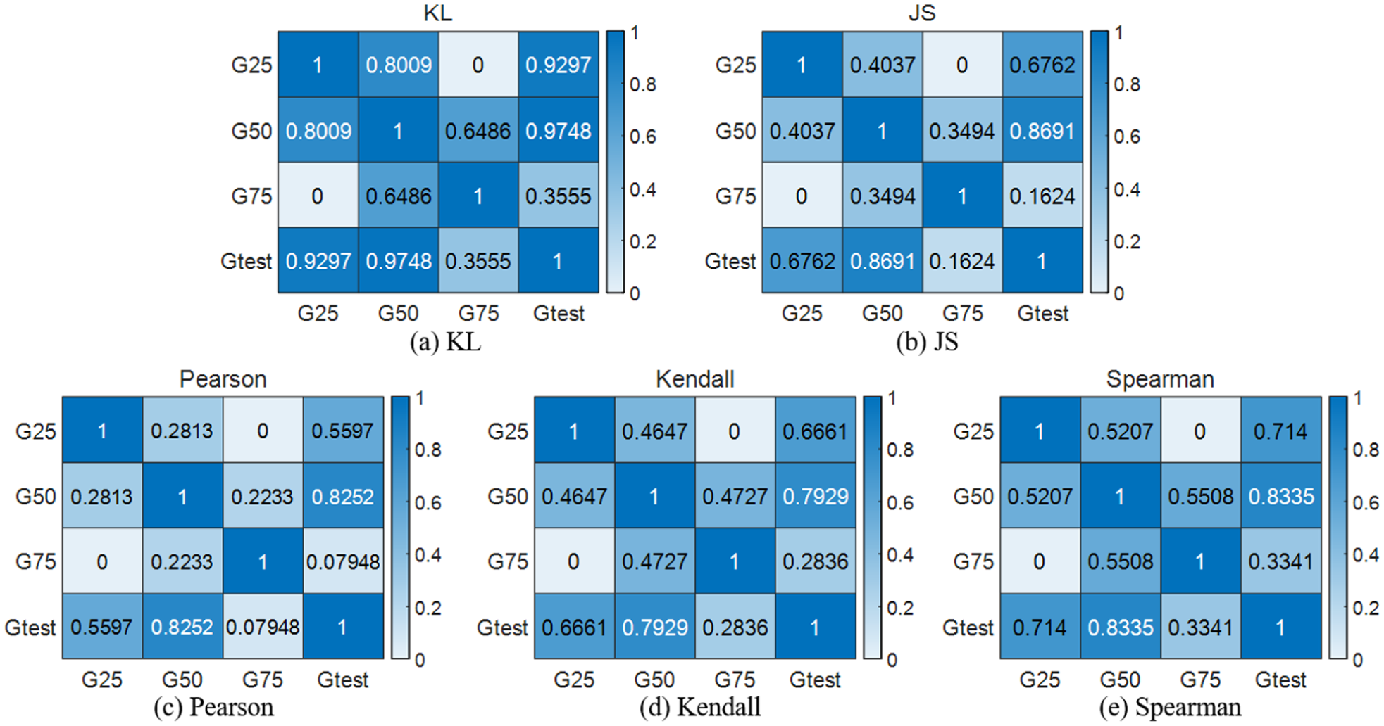
Correlation analysis results based on the IGAN model: (a) KL, (b) JS, (c) Pearson, (d) Kendall, and (e) Spearman.
Correlation analysis results based on the GANomaly model: (a) KL, (b) JS, (c) Pearson, (d) Kendall, and (e) Spearman.
Correlation analysis results based on the AE model: (a) KL, (b) JS, (c) Pearson, (d) Kendall, and (e) Spearman.
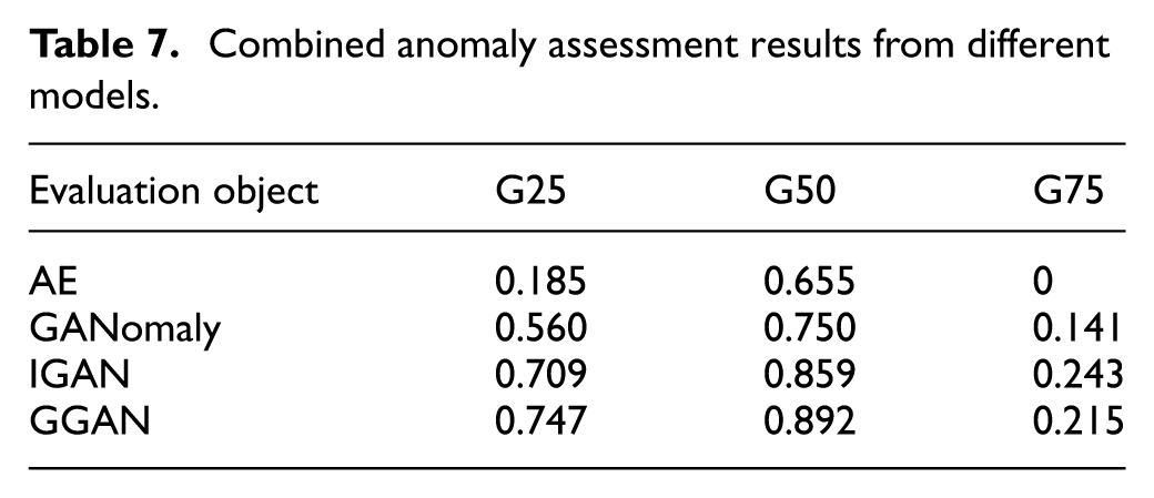
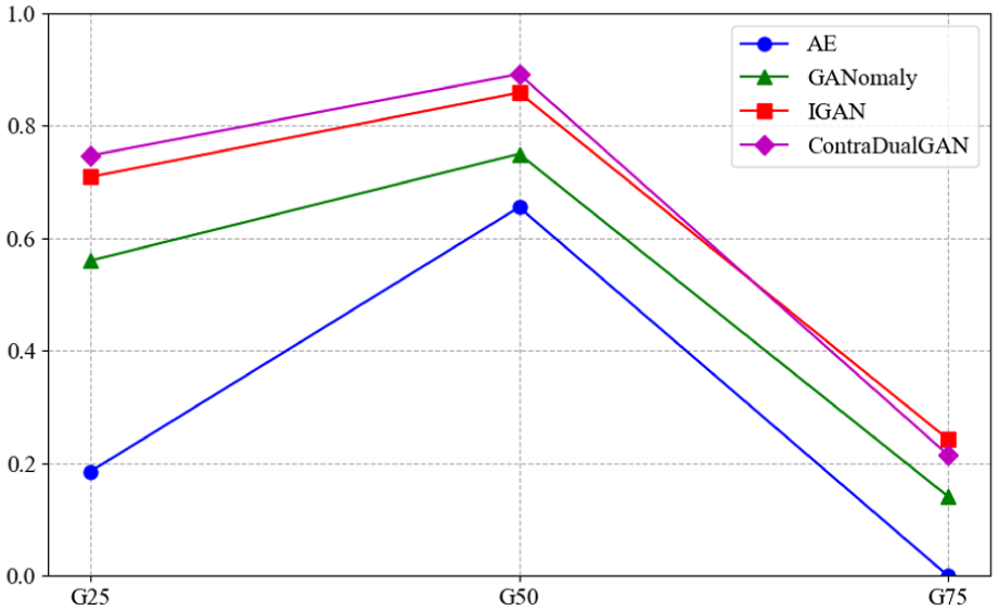
The integrated anomaly evaluation results of the different models are summarized in Table 7 and Figure 27. It can be seen that, among the results of the four models, G50 consistently achieves the highest integrated evaluation score, indicating that the fault-severity characteristics of the test data are most similar to G50, which is consistent with the ground truth.
Combined anomaly assessment results from different models.
Combined anomaly assessment results from different models.
Using the proposed anomaly evaluation framework, comparative experiments were conducted by replacing the anomaly detection model with different alternatives. The results show that all models can identify the fault severity of the test data. In particular, the GGAN model achieves an integrated evaluation score of 89.2%, outperforming the other methods and thereby validating the effectiveness of the proposed approach.
Summary
This paper develops a GGAN-based framework for anomaly assessment of gear transmission components. The framework consists of three stages. First, during normal operation, an anomaly detection model is established and trained exclusively on samples from the healthy condition. Second, when a small number of faults occur, the model is further trained using a limited set of abnormal samples, and the decision threshold is adjusted to improve detection accuracy. Third, when a large number of faults are available, data from various fault scenarios are used to characterize the anomaly scores of different faults. Subsequently, based on similarity analysis, anomaly assessment is performed by comparing the anomaly scores corresponding to different fault severity levels. To validate the assessment accuracy of the proposed framework, experiments were conducted on the XJTUSpurgear dataset and a self-built planetary gearbox fault-simulation test rig dataset, with comparative analyses against other classical models. The results demonstrate that all models can assess the severity of crack and tooth-breakage faults in the test data, while the GGAN model achieves a substantially higher integrated anomaly assessment score than the other three methods. These findings confirm the effectiveness of the proposed approach and provide a useful reference for practical engineering applications.
However, during the research process, we observed that the GGAN method proposed in this paper incurs certain computational overhead due to the integration of multiple modules. To balance performance and efficiency, future work can be optimized in two aspects: (1) In terms of model architecture, depthwise separable convolutions and lightweight attention mechanisms can be adopted to streamline the multi-scale discriminators and residual networks, while dynamic computational paths and feature-sharing mechanisms can be designed to reduce redundant operations. (2) In terms of training strategies, progressive multi-stage training can be introduced to stabilize the optimization process, and knowledge distillation techniques can be utilized to transfer the capabilities of the full model to a lightweight network, thereby significantly reducing computational load while maintaining anomaly detection accuracy.
Footnotes
Handling Editor: Yuansheng Zhou
Author contributions
Jian Shen: conceptualization, methodology, formal analysis, writing – original draft. Yingjie Zhao: supervision, resources, writing – review and editing. Peng Luo: software, validation, data curation, visualization, writing – original draft. Jiao Hu: investigation, validation, writing – review and editing.
Funding
The authors disclosed receipt of the following financial support for the research, authorship, and/or publication of this article: This work is financially supported by the Scientific Research Project of Education Department of Hunan Province (grant no. 23B1141) and the Natural Science Foundation of Hunan Province (grant no. 2024JJ8096).
Declaration of conflicting interests
The authors declared no potential conflicts of interest with respect to the research, authorship, and/or publication of this article.