Model-based MPC with adaptive weights for tracked vehicle trajectory tracking

Abstract

Trajectory tracking is crucial for intelligent tracked vehicles, with model predictive control (MPC) being a widely used method due to its ability to handle predictions and constraints. However, conventional MPC based on kinematic models neglects the coupled longitudinal–lateral dynamics, leading to limited accuracy and stability. To address this, we propose an MPC strategy that integrates both kinematic and dynamic models for dual-motor-driven tracked vehicles. This approach uses lateral deviation, heading deviation, longitudinal velocity, and yaw rate as state variables, with motor torques as control inputs, explicitly capturing dynamic coupling and electric drive characteristics. Additionally, we introduce a deep Q-network (DQN)-based adaptive weight adjustment scheme to improve disturbance rejection and overcome the limitations of fixed MPC weights. This adaptive mechanism optimizes the weight matrix online under varying operating conditions. The proposed method is validated through MATLAB/Simulink–RecurDyn co-simulation and low-speed vehicle tests, demonstrating significant improvements in trajectory tracking, with reductions in lateral and heading deviations by 58.4% and 18.6%, respectively. Further, the DQN-based adaptive weighting leads to additional improvements, reducing lateral and heading deviations by 36.6% and 19.7%.

Introduction

Tracked vehicles, with their superior off-road capability, high load capacity, low ground pressure, and zero-radius turning, are widely deployed in military, agricultural, engineering rescue, and emergency response applications. ¹ Compared with wheeled vehicles, dual-motor independently driven tracked vehicles differ significantly in drivetrain structure and steering mechanism: steering is achieved by generating speed or torque differences between the two tracks. Under real-world operating conditions, they exhibit pronounced longitudinal–lateral dynamic coupling, complex track–ground interactions, and high slip ratios, posing considerable challenges to high-precision trajectory tracking and maneuvering stability control.^2,3

The methods of trajectory tracking control mainly include pure tracking algorithm, ⁴ feedforward-feedback control, ⁵ PID control,^6,7 linear quadratic form (LQR), and model predictive control (MPC). In recent years, machine learning related algorithms have gradually been applied in the field of trajectory tracking control. ⁸ The pure tracking algorithm is based on the simplified steering kinematics model for trajectory tracking. It has small amount of calculation, can be combined with feedforward-feedback control, and has good trajectory tracking performance for low speed driving on smooth roads surfaces. The PID algorithm is simple, its parameters are easy to adjust, and it has strong robustness. It is only applicable to the decoupled linear time-invariant system, and has certain limitations in the application of nonlinear and high real-time system. The vehicle model in LQR is a linear time invariant system, and the control effect depends on an accurate mathematical model. It cannot guarantee robustness and stability under the condition of time-varying parameters or interference, and the trajectory tracking effect on sections with sudden curvature changes is poor. ⁹ Model predictive control (MPC) based on vehicle model can effectively solve multi-objective, multi constraint and multivariable optimization problems, with rolling optimization and feedback correction functions, can effectively reduce or even eliminate the impact of closed-loop system time-delay problems.^10–12 At present, the MPC is mostly used in intelligent wheeled vehicles to achieve trajectory tracking. Due to the significant differences in the transmission system structure between dual motor driven tracked vehicles and wheeled vehicles. Moreover, the tracked vehicle achieve steering by changing the speed or torque of the tracks on both sides, so the steering principle of tracked vehicles is very different from that of wheeled vehicles. The dynamics system of the tracked vehicle is a nonlinear time-varying system in both lateral and longitudinal directions. Therefore, the MPC is very suitable for the trajectory tracking control of tracked vehicles. At present, compared with wheeled vehicles, there is relatively little research on MPC trajectory tracking control for tracked vehicles.

The core content of MPC includes predictive model, rolling optimization, and feedback correction. The accuracy and complexity of the prediction model will affect the computational efficiency and trajectory tracking accuracy of tracked vehicles. In Li ¹³ and Zhou, ¹⁴ a trajectory tracking MPC controller based on the kinematics prediction model of the tracked vehicle is designed to track the trajectory by controlling the position deviation and heading angle deviation. Among them, the speeds of the left track and right track are the control variables. In Burke, ¹⁵ a kinematics prediction model without considering slip is proposed. The designed MPC controller uses track’s speed and the yaw rate as control variables to track vehicle position and heading angle. In Hu et al., ¹⁶ considering the effect of slip, the kinematics model of the tracked vehicle based on the instantaneous steering center is used as the prediction model, and the winding speeds of the left and right tracks are used as the control variables to achieve trajectory tracking, and the constraint expressions of the control variables and the state variables are given. Due to the lack of consideration for dynamics constraints, the trajectory tracking deviation in the above studies is significant. The prediction model in Tang et al., ¹⁷ Zhao et al., ¹⁸ and Lu et al. ¹⁹ is the same as that in Hu et al. ¹⁶ However, in Tang et al., ¹⁷ a dynamics analysis is conducted, the constraint values of the control variable for track winding speed are added, and the constraint of vehicle acceleration considering ground adhesion conditions is also added. The limit values of the speed control increment are defined, resulting in higher control accuracy for trajectory tracking. In Lu et al., ¹⁹ steering dynamics analysis was conducted. In order to ensure that tracked vehicle do not roll over, the speed constraints are set, and the longitudinal offset of the steering center is constrained to ensure that steering does not lose control, solving the problem of low trajectory tracking accuracy caused by the steering slip of the dual motor driven high-speed tracked vehicle in off-road condition. On the other hand, considering only the constraints of longitudinal velocity and acceleration cannot guarantee the lateral tracking accuracy of the tracked vehicle under many working conditions.

Recent studies have incorporated higher-fidelity models into MPC. Zhang et al. ²⁰ established a dynamic model of dual-motor-driven tracked vehicles that explicitly accounts for track–ground interaction and motor torque coupling, while Chen et al. ²¹ proposed a dynamic MPC framework capable of handling coupled dynamics and terrain uncertainty. Similarly, Elsharkawy et al. ²² analyzed the dynamic response of tracked vehicles under slope and nonuniform turning conditions, highlighting the necessity of accurate coupled modeling. These works confirm that dynamic-model-based MPC can significantly improve tracking performance under challenging operating conditions. In this paper, the MPC trajectory tracking control method that integrates the kinematics and dynamics prediction models will be proposed.

Another challenge is that MPC cost function weights are typically set empirically and remain fixed, which hinders adaptability across varying speeds, path curvatures, and adhesion levels. Adaptive methods such as fuzzy tuning or Bayesian optimization have been introduced,^23,24 but they either increase online computational burden or rely heavily on offline data with limited robustness. the current online parameter selection method for the MPC controller will to some extent increase the online calculation workload of the MPC, and some offline parameter optimization methods require a large amount of data information and cannot adapt to changing operating conditions. Reinforcement learning has significant advantages in online parameter optimization and has become a development trend at present.^25,26

Motivated by these challenges, this paper proposes a trajectory-tracking strategy that integrates a dynamic prediction model with MPC and introduces a deep Q-network (DQN)-based mechanism for online weight adaptation. The contributions are summarized as follows:

1. We develop a dynamic-model-based MPC framework for dual-motor-driven tracked vehicles, in which lateral deviation, yaw deviation, longitudinal velocity, and yaw rate are selected as state variables and track-side motor torques are used as control inputs. This enables the controller to explicitly account for longitudinal–lateral coupling and electric drive dynamics in both prediction and optimization.

2. We design a DQN-based adaptive weight adjustment scheme for the MPC cost function. Instead of relying on fixed or heuristically tuned weights, the proposed scheme learns an online mapping from vehicle states and reference information to the optimal weight matrix, thereby improving tracking accuracy and robustness under different speeds, curvatures, and adhesion levels.

3. The proposed approach is validated through MATLAB/Simulink–RecurDyn co-simulation and low-speed experiments, showing that dynamic-model-based MPC significantly outperforms kinematic MPC in terms of maximum lateral and yaw deviations, while DQN-based adaptation further enhances robustness and tracking performance.

Kinematics and dynamics modeling of tracked unmanned vehicle driven by dual motors

The electronic differential steering is adopted in a dual motor driven tracked vehicle, eliminating the need for mechanical or hydraulic steering control mechanism. By controlling the speed or torque of the motors on both sides, then the steering mode and mechanism are changed. In order to propose an effective model predictive trajectory control strategy, it is necessary to reconstruct the time-varying nonlinear kinematics and dynamics models of electronic differential steering. The schematic diagram of the chassis structure of the dual motor driven tracked vehicle is shown in Figure 1.

Figure 1.

Schematic diagram of the chassis structure of a dual motor driven tracked vehicle.

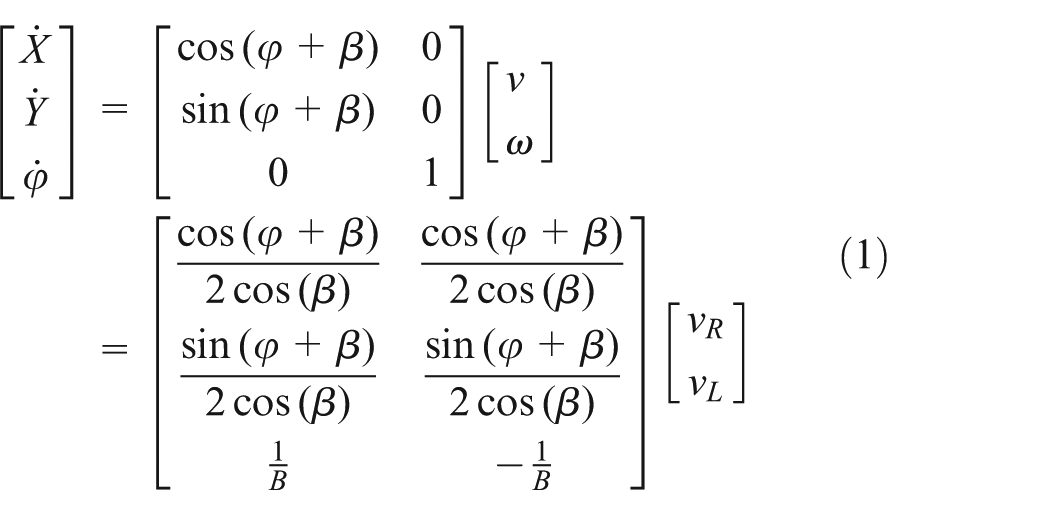
Steering kinematics analysis

As shown in Figure 2, the tracked vehicle may experience lateral sliding during the steering process, especially at high speeds (with speeds >0.8 rad/s), resulting in inconsistent speed direction with the body axis. In Figure 2, XOY is the global coordinate system, φ is the heading angle, β is the center of mass sideslip angle, o is the instantaneous turning center of the vehicle, v is the vehicle centroid velocity, R is the turning radius of the vehicle, and ω is the angular velocity, v _L is the axial linear speed at the outer track, n _L is the driving wheel speed, v _R is the axial linear speed of the inner track, n _R is the driving wheel speed; B is the center distance between the two tracks, L is the grounding length between the track and the ground, and r is the radius of the driving wheel.

Figure 2.

Kinematics analysis of tracked vehicles.

(O–XY) denotes the global coordinate frame, ψ is the heading angle, β is the sideslip angle at the vehicle center of mass, R is the turning radius, v is the centroid velocity, ω is the yaw rate, B is the track gauge, L is the track-grounding length.

Assuming a negligible change in β, which is valid for low to medium speed trajectory tracking and moderate curvature, where the sideslip angle β varies slowly and remains within a small range. In such cases, β can be treated as a bounded disturbance in the kinematic error dynamics. For higher-speed or more aggressive steering maneuvers, β is estimated online and explicitly incorporated into the dynamic prediction model as a measurable disturbance. A kinematics model of the tracked vehicle can be constructed as follows:

$$\begin{array}{c}\multicolumn{1}{c}{\left[\begin{array}{c}\stackrel{·}{X}\hfill \\ \multicolumn{1}{c}{\stackrel{·}{Y}}\\ \multicolumn{1}{c}{\stackrel{·}{\phi }}\end{array}\right]=\left[\begin{array}{cc}\cos (\phi +\beta )\hfill & 0\hfill \\ \multicolumn{1}{c}{\sin (\phi +\beta )}& 0\hfill \\ \multicolumn{1}{c}{0}& 1\hfill \end{array}\right]\left[\begin{array}{c}v\hfill \\ \multicolumn{1}{c}{\omega }\end{array}\right]}\\ \multicolumn{1}{c}{=\left[\begin{array}{cc}\frac{\cos (\phi +\beta )}{2\cos (\beta )}\hfill & \frac{\cos (\phi +\beta )}{2\cos (\beta )}\hfill \\ \multicolumn{1}{c}{\frac{\sin (\phi +\beta )}{2\cos (\beta )}}& \frac{\sin (\phi +\beta )}{2\cos (\beta )}\hfill \\ \multicolumn{1}{c}{\frac{1}{B}}& -\frac{1}{B}\hfill \end{array}\right]\left[\begin{array}{c}{v}_R\hfill \\ \multicolumn{1}{c}{v_L}\end{array}\right]}\end{array}$$

(1)

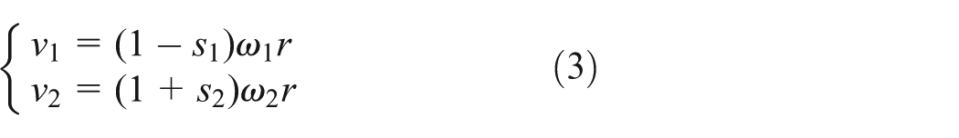
When analyzing the steering motion of the tracked vehicle, it is necessary to consider the sliding phenomenon of the tracks. The slip rate of the track can be expressed as follows:

$$\{\begin{array}{l}{s}_1=\frac{{\omega }_{1}r-v_1}{{\omega }_{1}r}\times 100\%\\ s_2=\frac{v_2-{\omega }_{2}r}{{\omega }_{2}r}\times 100\%\\ s_1\in (0,1),s_2\in (0,+\infty )\end{array}$$

(2)

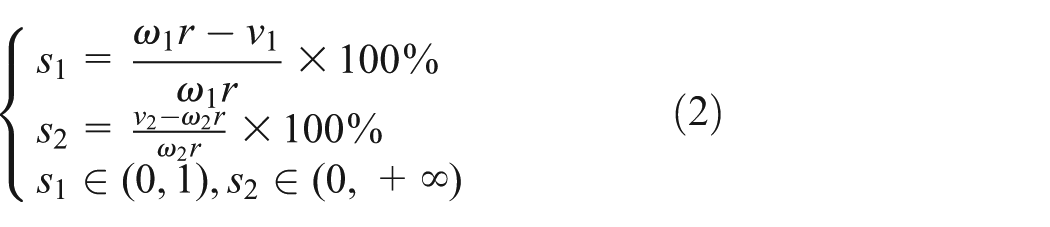
Where s₁ and s₂ represent the slip rates of the outer and inner tracks, ω₁ and ω₂ represent the angular velocities of the outer and inner drive wheels, and v₁ and v₂ represent the axial linear speeds of the outer and inner wheels, respectively.

So the relationship between v₁, v₂ and ω₁, ω₂ is:

$$\{\begin{array}{c}{v}_1=(1-s_1){\omega }_{1}r\hfill \\ \multicolumn{1}{c}{v_2=(1+s_2){\omega }_{2}r}\end{array}$$

(3)

If $\tilde{s}=\frac{v}{\omega r}-1$ is defined, then equation (3) can be uniformly expressed as:

$$v=(1+\tilde{s})\omega r$$

(4)

By substituting the equation (3) into the equation (4), the following expression can be obtained as followed:

$$\left[\begin{array}{c}\stackrel{·}{x}\hfill \\ \multicolumn{1}{c}{\stackrel{·}{y}}\\ \multicolumn{1}{c}{\stackrel{·}{\phi }}\end{array}\right]=\left[\begin{array}{cc}\frac{\cos (\phi +\beta )}{2\cos (\beta )}\hfill & \frac{\cos (\phi +\beta )}{2\cos (\beta )}\hfill \\ \multicolumn{1}{c}{\frac{\sin (\phi +\beta )}{2\cos (\beta )}}& \frac{\sin (\phi +\beta )}{2\cos (\beta )}\hfill \\ \multicolumn{1}{c}{\frac{1}{B}}& -\frac{1}{B}\hfill \end{array}\right]\left[\begin{array}{c}(1+{\tilde{s}}_R)r{\omega }_R\hfill \\ \multicolumn{1}{c}{(1+{\tilde{s}}_L)r{\omega }_L}\end{array}\right]$$

(5)

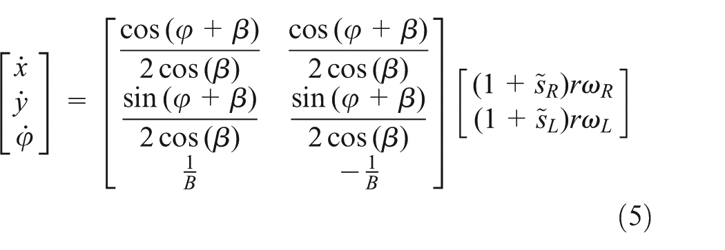
Where the sliding parameters can be estimated and obtained from the state feedback $\tilde{s}$ . In our implementation, an extended Kalman filter (EKF) referencing the standard formulation in Rajamani ²⁷ is used to estimate β and slip-related states from measured longitudinal speed, yaw rate and left/right motor angular speeds; the EKF outputs are then supplied to the dynamic prediction model and MPC constraints. The relationship between the winding speed of the tracks and the speed of the drive motors on both sides is expressed as follows:

$${\omega }_i=\frac{2\pi n_i}{60000i}=0.377\frac{n_i}{i}$$

(6)

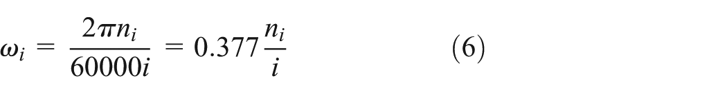
Where, i is the reduction ratio from the motor to the driving wheel.

Dynamics analysis during straight-line driving

The force balance equation for the straight-line traveling of the tracked vehicle is as follows:

$$\begin{array}{c}{F}_t=F_f+F_i+F_w+F_j\hfill \\ =\mathrm{fG}+G\sin \alpha +\frac{C_{D}A}{21.15}{v}^2+\delta M\frac{\mathrm{dv}}{\mathrm{dt}}\hfill \end{array}$$

(7)

Where G is the total vehicle weight (N), M is the vehicle mass (kg), F _t is the required traction force of the entire vehicle (N), $F_f$ is the driving resistance of the tracked vehicle (N), f is the road resistance coefficient, F _i is the gradient resistance (N), F _w is the air resistance (N), C _D is the air drag coefficient, A is the front windward area of the vehicle $(m^2)$ , F _j is the acceleration resistance $(N),\delta$ is the coefficient of the revolving mass.

The F _t required for the entire vehicle is limited by the output torque $[T_{\min },T_{\max }]$ of the drive motors on both sides of the tracked vehicle. It is known that the reduction ratio of the reducer is i, the transmission efficiency is η, and the radius of the driving wheel is r. Then the following expression can be obtained as followed:

$$F_t=\frac{\mathrm{Ti}\eta }{r}$$

(8)

Dynamic analysis during steering

By adjusting the driving torque of the two motors on both sides to regulate the speed of the tracks on both sides, the tracked vehicle can achieve steering motion. The drive motor can operate in four quadrants, and the typical steering conditions for the dual motor independent drive tracked vehicle are shown in Figure 3.

Figure 3.

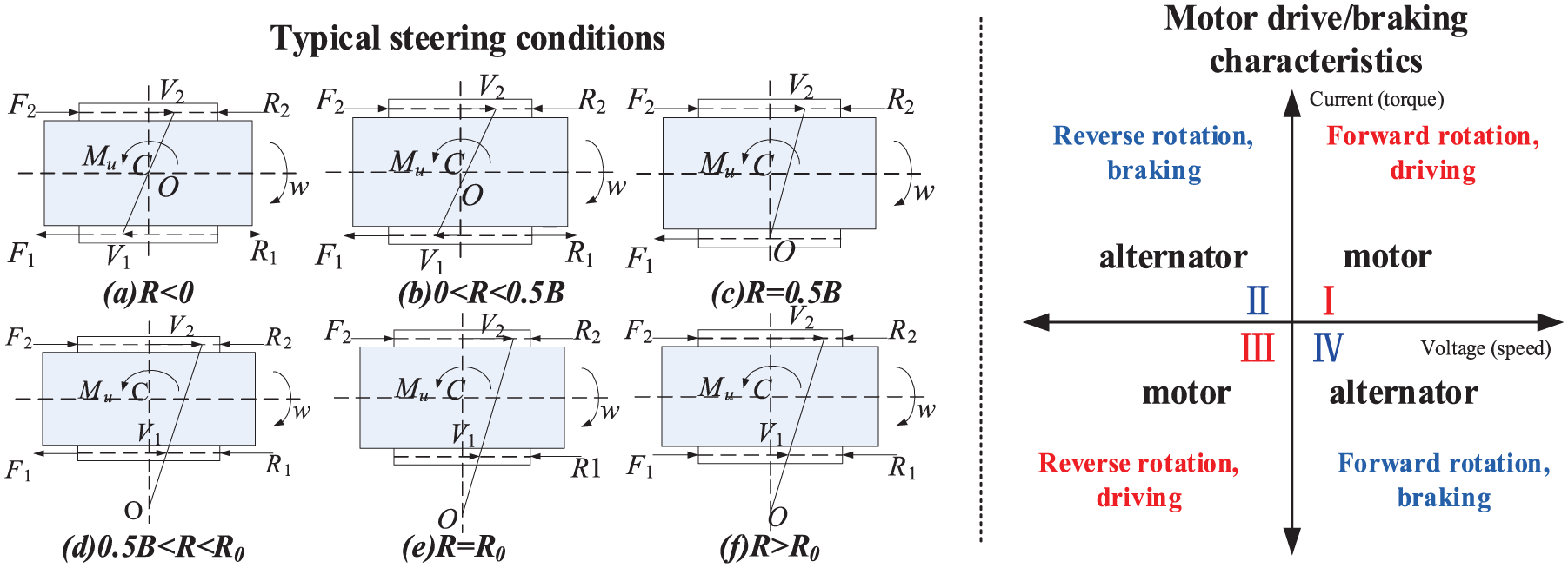
The typical steering conditions for the dual motor independent drive tracked vehicle and the operating characteristics of the four quadrants of the motor.

As shown in Figure 4, the steering speed of the tracks on both sides is different, and the direction of the longitudinal friction force F _fi is opposite to the direction of the track speed, namely:

$$\{\begin{array}{c}{F}_{\mathrm{fi}}=\mathrm{sign}(V_i)F_f\hfill \\ \multicolumn{1}{c}{F_f=\frac{\mu \mathrm{mg}}{2}}\end{array}$$

(9)

Where, μ is the friction resistance coefficient between the track and the ground. sign is a Sign function:

$$\{\begin{array}{c}\mathrm{sign}(V_i)=1,V_i>0\hfill \\ \multicolumn{1}{c}{\mathrm{sign}(V_i)=0,V_i=0}\\ \multicolumn{1}{c}{\mathrm{sign}(V_i)=-1,V_i<0}\end{array}$$

Figure 4.

Schematic diagram of steering force analysis for the tracked vehicle: (a) turning at low speed and (b) turning at high speed.

According to the normal load per unit length on the grounding area of the track, the lateral friction resistance of the corresponding grounding area track can be obtained.

The friction coefficient between the track and the ground is μ, which is approximately equal to the friction coefficient between the track shoe and the ground. The normal load per unit length on the connecting section is p. d is the distance at which the center of mass shifts during high-speed turning. The lateral frictional resistance of the front and rear sections of the track during steering can be expressed as:

$$\{\begin{array}{c}{F}_{\mathrm{yf}1}=F_{\mathrm{yf}2}={\int }_0^{\frac{L}{2}-d}\mu \mathrm{pdx}=\frac{\mu G}{2L}(\frac{L}{2}-d)\hfill \\ \multicolumn{1}{c}{F_{\mathrm{yr}1}=F_{\mathrm{yr}2}={\int }_0^{\frac{L}{2}+d}\mu \mathrm{pdx}=\frac{\mu G}{2L}(\frac{L}{2}+d)}\end{array}$$

(10)

The steering resistance moment M _y caused by the lateral frictional resistance is:

$$M_y=\frac{\mu \mathrm{GL}}{4}[1+{\left(\frac{2d}{L}\right)}^2]$$

(11)

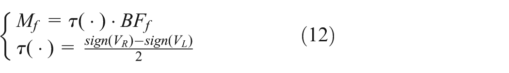
The resistance moment M _f caused by longitudinal friction is expressed as:

$$\{\begin{array}{c}{M}_f=\tau (·)·B{F}_f\hfill \\ \multicolumn{1}{c}{\tau (·)=\frac{\mathrm{sign}(V_R)-\mathrm{sign}(V_L)}{2}}\end{array}$$

(12)

Neglecting centrifugal force, the total steering resistance moment of tracked vehicles during steering M _zu is:

$$M_{\mathrm{zu}}=\frac{\mu \mathrm{GL}}{4}+\tau (·)B{F}_f$$

(13)

The constraint expression for the resistance coefficient is as follows:

$${\mu }_{min}<\mu <{\mu }_{max}$$

(14)

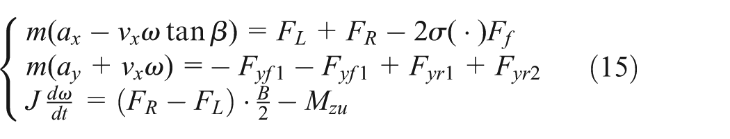
According to Newton’s Second Law, the lateral, longitudinal, and yaw movements during track steering can be expressed as:

$$\{\begin{array}{c}m(a_x-v_x\omega \tan \beta )=F_L+F_R-2\sigma (·)F_f\hfill \\ \multicolumn{1}{c}{m(a_y+v_x\omega )=-F_{\mathrm{yf}1}-F_{\mathrm{yf}1}+F_{\mathrm{yr}1}+F_{\mathrm{yr}2}}\\ \multicolumn{1}{c}{J\frac{d\omega }{\mathrm{dt}}=(F_R-F_L)·\frac{B}{2}-M_{\mathrm{zu}}}\end{array}$$

(15)

Where, $\sigma (·)=\frac{\mathrm{sgn}(V_L)+\mathrm{sgn}(V_R)}{2}$

f is defined as the coefficient of vehicle driving resistance. By substituting the equations (9), (10), and (13) into the equation (15), the following expression can be obtained:

$$\{\begin{array}{c}{\stackrel{·}{v}}_x=\frac{F_L+F_R}{m}-\sigma (·)\mathrm{fg}+v_x\omega \tan \beta \hfill \\ \multicolumn{1}{c}{{\stackrel{·}{v}}_y=-v_x\omega }\\ \multicolumn{1}{c}{\stackrel{·}{\omega }=\frac{1}{J}(F_R-F_L)·\frac{B}{2}-\frac{{\mu }_x\mathrm{GL}}{4}+\tau (·)B{F}_f}\end{array}$$

(16)

Preview trajectory tracking MPC control strategy

Model predictive control (MPC)

The design of a model predictive controller includes three parts: establishing a predictive model, constructing a objective function and obtaining the optimal control quantities. The design process is shown in Figure 5.

Figure 5.

MPC design framework.

In the Figure 5, y(t) is the actual output of the controlled object at the current time, T is the sampling period of the MPC controller, N _p is the predictive time domain, N _c is the control time domain, $Y_{\mathrm{ref}}(t)$ is the output reference value of the system, $U\left(t\right)=[u(t|t),u(t+1|t),\cdots u(t+N_c-1|t){]}^T$ is the optimal control variables in N _c , and $Y\left(t\right)=[y(t+1|t{)}^T\cdots y(t+N_p|t{)}^T{]}^T$ is the predicted output variables in N _p .

According to the feedback current state estimation value $x^{*}(t)$ , the disturbance variables w(t), U(t) and Y(t) are obtained through the prediction model. Combined with $Y_{\mathrm{ref}}(t)$ , The objective function is constructed, the constraint conditions are designed and the optimization solution is being carried out. The first optimized control quantity $u(t+1|t+1)$ of $U(t+1)$ is input into the controlled system, and then the next time step operation for optimization solution begins. By repeating the above process, rolling optimization, and feedback control can be achieved.

The MPC based on kinematics of tracked vehicles

The establishment and discretization of prediction models

According to Figure 2, the preview characteristics of the driver are first considered. The preview distance constant is set to L _d , and the reference trajectory P _ref is founded. Its coordinates in its global coordinate system are $(X_{\mathrm{ref}},Y_{\mathrm{ref}})$ , and the expected longitudinal velocity at this point P _ref is v _d . The curvature and tangential angle of the reference trajectory at this point P _ref are ρ and φ _ref , respectively.

From the Figure 2, the state equation of the error model is obtained as follows:

$$\{\begin{array}{c}{\stackrel{·}{y}}_e=v_x{\phi }_e-\omega L_d\hfill \\ \multicolumn{1}{c}{{\stackrel{·}{\phi }}_{\mathrm{e}}=v_x\rho -\omega }\end{array}$$

(17)

The lateral deviation y _e and the heading angle deviation φ _e are selected as the state variables, with the yaw rate ω as the control variable. v _x is the actual longitudinal speed at the current moment, the curvature of the reference point ρ is selected as the measurable disturbance, y _e and φ _e are selected as the output variables. The equation (17) is written in the form of state space and expressed as follows:

$$\{\begin{array}{c}\stackrel{·}{x}=\mathrm{Ax}+\mathrm{Bu}+\mathrm{Dw}\hfill \\ \multicolumn{1}{c}{y=\mathrm{Cx}}\end{array}$$

(18)

Where $x={[y_e,{\phi }_e]}^T,u=\omega ,w=\rho$ , the coefficient matrix in equation (18) are set as follows:

$$\begin{array}{c}A=\left[\begin{array}{cc}0\hfill & v_x\hfill \\ \multicolumn{1}{c}{0}& 0\hfill \end{array}\right],B=\left[\begin{array}{c}-L_d\hfill \\ \multicolumn{1}{c}{-1}\end{array}\right];\hfill \\ D=\left[\begin{array}{c}0\hfill \\ \multicolumn{1}{c}{v_x}\end{array}\right],C=\left[\begin{array}{cc}1\hfill & 0\hfill \\ \multicolumn{1}{c}{0}& 1\hfill \end{array}\right].\hfill \end{array}$$

The continuous state space equation of the equation (17) is discretized and represented as follows:

$$\{\begin{array}{c}x(k+1)=A_{\mathrm{kt}}x(k)+B_{\mathrm{kt}}u(k)+D_{\mathrm{kt}}w(k)\hfill \\ \multicolumn{1}{c}{y(k)=C_{\mathrm{kt}}x(k)}\\ \multicolumn{1}{c}{u(k)=u(k-1)+\Delta u(k)}\end{array}$$

(19)

Where, $A_{\mathrm{kt}}=e^{\mathrm{AT}}$ , $B_{\mathrm{kt}}={\int }_0^T{e}^{\mathrm{AT}}d\tau ·B$ , $D_{\mathrm{kt}}={\int }_0^T{e}^{\mathrm{AT}}d\tau ·D$ , $C_{\mathrm{kt}}=C$ .

Furthermore, in order to improve computational efficiency, the above parameters are simplified:

$$\{\begin{array}{c}{A}_{\mathrm{kt}}=A_{\mathrm{tt}},k=1,2,\dots ,t+N_p-1\hfill \\ \multicolumn{1}{c}{B_{\mathrm{kt}}=B_{\mathrm{tt}},k=1,2,\dots ,t+N_p-1}\end{array}$$

(20)

In summary, the output equation of the entire discrete system at time t is:

$$Y(t)=\tilde{A}x(t)+{\tilde{B}}_{u}u(t-1)+{\tilde{B}}_{\Delta U}\Delta U(t)+\tilde{D}W(t)$$

Where,

$$\begin{array}{c}Y(t)=[y(t+1|t{)}^T,\cdots ,y(t+N_P|t{)}^T{]}^T\hfill \\ \Delta U(t)=[\Delta u(t|t{)}^T,\cdots ,\Delta u(t+N_C-1|t{)}^T{]}^T,\hfill \\ W(t)=[w(t|t{)}^T,\cdots ,w(t+N_P-1|t{)}^T{]}^T,\hfill \\ \tilde{A}=[A_{\mathrm{kt}},A_{\mathrm{kt}}^2,\dots ,A_{\mathrm{kt}}^{N_C},\dots ,A_{\mathrm{kt}}^{N_P}{]}^T,\hfill \\ \tilde{B}=[B_{\mathrm{kt}},\dots ,\sum _{i=0}^{N_C}{A}_{\mathrm{kt}}^i{B}_{\mathrm{kt}},\dots ,\sum _{i=0}^{N_P-1}{A}_{\mathrm{kt}}^i{B}_{\mathrm{kt}}{]}^T,\hfill \end{array}$$

$$\begin{array}{c}{\tilde{B}}_{\Delta U}=\left[\begin{array}{ccc}{B}_{\mathrm{kt}}\hfill & \cdots \hfill & 0\hfill \\ \multicolumn{1}{c}{⋮}& \ddots \hfill & ⋮\hfill \\ \multicolumn{1}{c}{\sum _{i=0}^{N_C-1}{A}_{\mathrm{kt}}^i{B}_{\mathrm{kt}}}& \cdots \hfill & A_{\mathrm{kt}}{B}_{\mathrm{kt}}+B_{\mathrm{kt}}\hfill \\ \multicolumn{1}{c}{⋮}& \hfill & ⋮\hfill \\ \multicolumn{1}{c}{\sum _{i=0}^{N_P-1}{A}_{\mathrm{kt}}^i{B}_{\mathrm{kt}}}& \cdots \hfill & \sum _{i=0}^{N_P-N_C}{A}_{\mathrm{kt}}^i{B}_{\mathrm{kt}}\hfill \end{array}\right],\hfill \\ \tilde{D}=\left[\begin{array}{cccc}{D}_{\mathrm{kt}}\hfill & 0\hfill & \cdots \hfill & 0\hfill \\ \multicolumn{1}{c}{A_{\mathrm{kt}}{D}_{\mathrm{kt}}}& D_{\mathrm{kt}}\hfill & \cdots \hfill & 0\hfill \\ \multicolumn{1}{c}{⋮}& ⋮\hfill & \ddots \hfill & 0\hfill \\ \multicolumn{1}{c}{A_{\mathrm{kt}}^{N_P-1}{D}_{\mathrm{kt}}}& A_{\mathrm{kt}}^{N_P-2}{D}_{\mathrm{kt}}\hfill & \cdots \hfill & D_{\mathrm{kt}}\hfill \end{array}\right].\hfill \end{array}$$

When $N_C<t\le N_p$ , the change in output is 0, $u(t+N_C+j|t)=u(t+N_C|t)$ .

The selection of N _P has a great impact on the accuracy of trajectory tracking control, and N _C is directly related to the dimension of the optimal control sequence, which affects the calculation efficiency. In this paper, according to the equations (21) and (22), N _P is selected as 15 and N _C is selected as 3, which have been also adjusted by simulation test.

$$\frac{p_a{t}_F}{T}\le N_P\le \frac{t_F}{T}$$

(21)

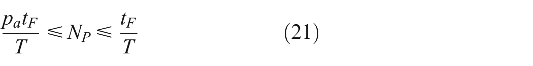
According to different controlled objects, P_a is generally set as 1/4–1/3, t_F is the system dynamics response time.

$$N_C\in \{0.1N_P\le N_C\le 0.2N_P\}\cap \{3\le N_C\}$$

(22)

Objective function and constraints

Firstly, in order to improve the trajectory tracking accuracy of the controller, it is desired that the lateral deviation and heading angle deviation of the controlled vehicle tend to zero. The objective function is set as follows:

$$J_1=\sum _{i=1}^{N_P}[||y_e(t+i|t)-y_{e\_\mathrm{ref}}(t+i|t)|{|}_{Q_{y_e}}^2+||{\phi }_e(t+i|t)-{\phi }_{e\_\mathrm{ref}}(t+i|t)|{|}_{Q_{{\phi }_e}}^2]$$

(23)

Where, $y_{e\_\mathrm{ref}}=0,{\phi }_{e\_\mathrm{ref}}=0$ , $Q_{y_e}$ and $Q_{{\phi }_e}$ are the weight values used to describe the lateral deviation and the heading angle deviation, respectively.

The equation (13) is written in matrix form as follow:

$$J_1=||Y(t)-Y_{\mathrm{ref}}(t)|{|}_Q^2$$

(24)

Where, $Y=[y_e,{\phi }_e{]}^T$ , $Y=[y_{e\_\mathrm{ref}},{\phi }_{e\_\mathrm{ref}}{]}^T$ ,

$$Q=[Q_{y_e},Q_{{\phi }_e}{]}^T.$$

In addition, it is usually necessary to take into account the rate of change of the control variable, and the second term of the objective function is set to:

$$\underset{\Delta U}{min{J}_2}=\Vert \Delta U(t){\Vert }_R^2$$

(25)

Where, R is the weight matrix of the MPC controller control term. J₂ is generally used to describe the comfort level of riding, but the rate of change of the control variable can also affect the control effect to some extent. For example, an excessively large rate of change of the control variable can easily lead to overshoot during trajectory tracking.

Combining J₁ and J₂, the objective function of the model predictive controller is designed as follows:

$$\underset{\Delta U}{minJ}=\Vert Y(t)-Y_{\mathrm{ref}}(t){\Vert }_Q^2+\Vert \Delta U(t){\Vert }_R^2+\sigma {\epsilon }^2$$

(26)

Where, $Y_{\mathrm{ref}}(t)=[y_{\mathrm{ref}}(t+1|t{)}^T,\cdots ,y_{\mathrm{ref}}(t+N_P|t{)}^T{]}^T$ is the expected output (i.e. expected lateral deviation, expected heading deviation), δ is the weight coefficient, and ε is the relaxation factor.

This objective function combines three tasks. The first task is to ensure the tracking accuracy of the predicted output reference value, that is, the desired path. The second task is to ensure that the change in control increment is as small as possible to ensure the smooth turning behavior of the vehicle. The third task is a relaxation term.

Due to the lack of consideration of dynamics factors and motor characteristics in the kinematics model, only soft constraints are applied to state variables and control variables:

$$y_{e\_min}\le y_e\le y_{e\_max}$$

(27)

$${\phi }_{e\_min}\le {\phi }_e\le {\phi }_{e\_max}$$

(28)

$${\omega }_{min}\le \omega \le {\omega }_{max}$$

(29)

Where, the lateral deviation at each moment shall not be too large, which is taken as $\left|y_{e\_\min }\right|=\left|y_{e\_\min }\right|=1.5m$ , and the heading angle deviation shall also be kept in a small range to meet the small angle hypothesis, $\left|{\phi }_{e\_\min }\right|=\left|{\phi }_{e\_\min }\right|=0.52\mathrm{rad}$ . The extreme value of yaw rate is determined by the current vehicle speed, the curvature of the reference point, and the performance of the controlled vehicle, namely $|{\omega }_{\min }|=\left|{\omega }_{\max }\right|=\left|v_x\rho \right|$ .

The optimal solution

The objective function is solved by the quadratic programming algorithm, and the equation (26) is transformed into the following standard quadratic function as followed:

$$J=\frac{1}{2}{\left[\begin{array}{c}\Delta U\hfill \\ \multicolumn{1}{c}{\epsilon }\end{array}\right]}^T\Theta \left[\begin{array}{c}\Delta U\hfill \\ \multicolumn{1}{c}{\epsilon }\end{array}\right]+\Xi \left[\begin{array}{c}\Delta U\hfill \\ \multicolumn{1}{c}{\epsilon }\end{array}\right]$$

(30)

From the equation (30), the optimal control increment sequence $\Delta U(t)$ is obtained, and the sum of the first item of the sequence and the current control variable is selected as the next long control variable. By using the multi-objective optimization with constraints, the optimal control sequence can be obtained by rolling optimization in real time.

The MPC based on dynamics of tracked vehicles

The establishment and discretization of prediction models

The kinematic preview model in equation (17) provides the path-related error states, including the lateral deviation y _e and the heading deviation φ _e , whereas the dynamic model in equation (16) captures the coupled longitudinal–lateral dynamics through the longitudinal velocity v _x and the yaw rate ω. In the proposed controller, these four quantities are stacked into an augmented state vector.

Based on the kinematics analysis of the tracked vehicle steering in Section 2, the prediction equation based on dynamics is constructed as follows:

$$\{\begin{array}{c}{\stackrel{·}{y}}_e=v_x{\phi }_e+v_x\tilde{\beta }-\omega L_d\hfill \\ \multicolumn{1}{c}{{\stackrel{·}{\phi }}_{\mathrm{e}}=v_x\rho -\omega }\\ \multicolumn{1}{c}{\stackrel{·}{\omega }=\frac{i\eta B}{2\mathrm{rJ}}(T_R-T_L)-\frac{M_z+\tau (·)B{F}_f}{J}}\\ \multicolumn{1}{c}{{\stackrel{·}{v}}_x=\frac{i\eta }{r}(T_R+T_L)+v_x\omega \tilde{\beta }+\frac{2\sigma (·)F_f}{m}}\end{array}$$

(31)

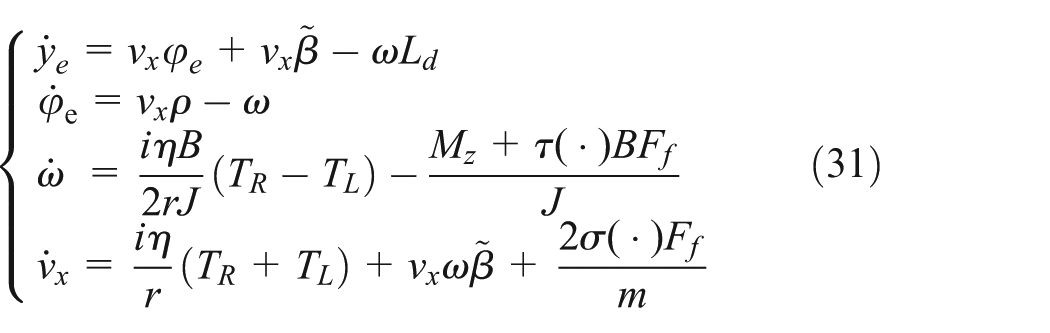
Where the y _e , φ _e , ω, and v _x are selected as the state variables, the driving torque $[T_R,T_L]$ of the motors on both sides is taken as the control variable, $\sigma (·),\tau (·)$ , the curvature ρ at the reference point and the real-time estimated sideslip angle $\tilde{\beta }$ of the center of mass are taken as the measurable disturbance variables, and y _e , φ _e , and v _x are selected as the output variables. The nonlinear dynamics state space equation for trajectory tracking control is established as follows:

$$\{\begin{array}{c}\stackrel{·}{\xi }=f(\xi ,u,d_{\_m})\hfill \\ \multicolumn{1}{c}{\eta =h\left(\xi \right)}\end{array}$$

(32)

Where, $\xi ={[y_e,{\phi }_e,\omega ,v_x]}^T$ , $u=[\begin{array}{cc}{T}_R\hfill & T_L\hfill \end{array}{]}^T$ , $d_{\_m}={[\sigma ,\tau ,\rho ,\tilde{\beta }]}^T$ , $\eta ={[y_e,{\phi }_e,v_x]}^T$ .

Since the dynamic model (equation (32)) is nonlinear, a successive linearization strategy is adopted. At each sampling instant, the model is linearized around the current state and input, $(x_k,u_k)$ using Jacobian matrices.

$$A_k={\frac{\partial f(x,u)}{\partial x}|}_{x_k,u_k},B_k={\frac{\partial f(x,u)}{\partial u}|}_{x_k,u_k}$$

(33)

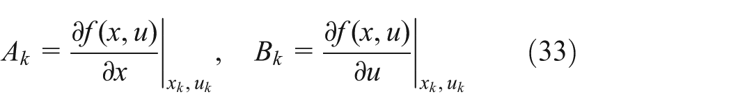
The resulting local linear time-varying (LTV) model is then discretized via the backward difference method and used as the prediction model in the MPC formulation.

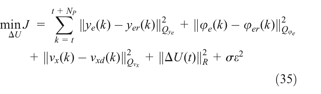
Objective function construction and constraints

Due to the use of a transverse and longitudinal coupling control strategy, the tracking target variables and predicted output variables not only contain lateral deviation and heading angle deviation, but also longitudinal velocity, that is, $\eta ={[y_e,{\phi }_e,v_x]}^T$ . Therefore, the corresponding reference value is ${\eta }_{\mathrm{ref}}={[y_{\mathrm{er}},{\phi }_{\mathrm{er}},v_{\mathrm{xd}}]}^T$ , and the reference value in each predicted time domain is $Y_{\mathrm{ref}}(t)=[{\eta }_{\mathrm{ref}}(t+1|t{)}^T,\cdots ,{\eta }_{\mathrm{ref}}(t+N_P|t{)}^T{]}^T$ .

The objective function of the trajectory tracking control based on dynamics prediction model is:

$$\underset{\Delta U}{minJ}=\Vert Y(t)-Y_{\mathrm{ref}}(t){\Vert }_Q^2+\Vert \Delta U(t){\Vert }_R^2+\sigma {\epsilon }^2$$

(34)

Where, $Q=[Q_{y_e},Q_{{\phi }_e},Q_{v_e}]$ is the weight coefficient. It can also be written in the following form:

$$\begin{array}{c}\underset{\Delta U}{minJ}=\sum _{k=t}^{t+N_P}\Vert y_e(k)-y_{\mathrm{er}}(k){\Vert }_{Q_{y_e}}^2+\Vert {\phi }_e(k)-{\phi }_{\mathrm{er}}(k){\Vert }_{Q_{{\phi }_e}}^2\hfill \\ +\Vert v_x(k)-v_{\mathrm{xd}}(k){\Vert }_{Q_{v_x}}^2+\Vert \Delta U(t){\Vert }_R^2+\sigma {\epsilon }^2\hfill \end{array}$$

(35)

Next, the constraints of the trajectory tracking MPC controller are established and include output constraints, control increment constraints, and state variable constraints. The constraints on state variables and output variables are similar to equations (25) to (27).

The constraints on control variables need to be combined with the mechanical structure of the tracked vehicle based on motor characteristics, and the driving torque $[T_R,T_L]$ needs to meet the following requirements:

$$\{\begin{array}{c}{T}_{Rmin}\le T_R\le T_{Rmax}\hfill \\ \multicolumn{1}{c}{T_{Lmin}\le T_L\le T_{Lmax}}\end{array}$$

(36)

Where, $i\in \{R,L\}$ and T _imax should not exceed the peak driving torque T _m calibrated by the motor, but also meet the power constraints of the motor, namely:

$$T_i\le 9549\frac{P_m}{n_i}$$

(37)

So, ${\left|T_i\right|}_{max}=min(T_m,9549\frac{P_m}{n_i})$ .

Taking all the constraints established above into account, the equation (34) is simplified into the standard form of Quadratic programming:

$$\{\begin{array}{c}\underset{\Delta U\in R^m}{min}J(\Delta U)=\frac{1}{2}\Delta U^T\Theta \Delta U+\Psi \Delta U\hfill \\ \multicolumn{1}{c}{s.t.y_{e\_min}\le y_e\le y_{e\_max},}\\ \multicolumn{1}{c}{{\phi }_{e\_min}\le {\phi }_e\le {\phi }_{e\_max},}\\ \multicolumn{1}{c}{{\omega }_{min}\le \omega \le {\omega }_{max},}\\ \multicolumn{1}{c}{\left|T_R\right|\le {\left|T_R\right|}_{max},\left|T_L\right|\le {\left|T_L\right|}_{max}.}\end{array}$$

(38)

Finally, the solution of the optimal output torque increment sequence is completed. The first term is taken and added to the control variable at t−1 to obtain the optimal control variable at t, which is then output to the controlled vehicle for control.

The optimal control quantity can be determined by minimizing the objective function (equation (37)) while satisfying the constraints. This process can be transformed into a Convex optimization problem under the constraints and solved by the Quadratic programming method.

The final control strategy structure block diagram proposed is shown in Figure 6.

Figure 6.

MPC-based trajectory tracking control framework with DQN-based weight adaptation.

Adaptive adjustment method of objective function weight matrix based on DQN

The Q-learning algorithm is a classic algorithm in traditional reinforcement learning. By continuously interacting with the environment, the agents learn better behavioral strategies and gradually update and improve the state action table (Q-table). The value of the table represents the maximum expected reward that can be obtained when executing an action in a certain state. However, when the environment dimension of the agent is high and there are many states, the continued use of Q-table to store the state action value function will cause a “Curse of dimensionality.”

To address this issue, the DeepMind team have integrated the deep neural networks with the Q-learning algorithm and proposed the deep Q network (DQN) algorithm. The DQN algorithm is an improvement on the Q-learning algorithm, which utilizes a deep neural network to dynamically generate a Q-value table and approximates the state action value function by continuously iterating and updating the parameters θ of the neural network f. The goal of parameter learning in the DQN algorithm mentioned above depends on the parameters themselves, which also leads to the Q network becoming more inclined towards actions with originally high Q values, resulting in the instability of the algorithm. To solve this problem, the double deep Q network (DDQN) can add a target Q network on top of the original DQN algorithm. The DDQN algorithm process is shown in Figure 7.

Figure 7.

DDQN algorithm training process with experience playback area.

The objective of this study is to calculate the optimal control quantity based on the feedback information from tracked vehicles and the reference trajectory and speed established in the previous planning layer, in order to obtain the optimal tracking accuracy. The solution of the optimal control sequence in MPC strategy is transformed into a quadratic programming problem.

Therefore, the task of solving the optimal control quantity within each time step can be divided into two small subtasks:

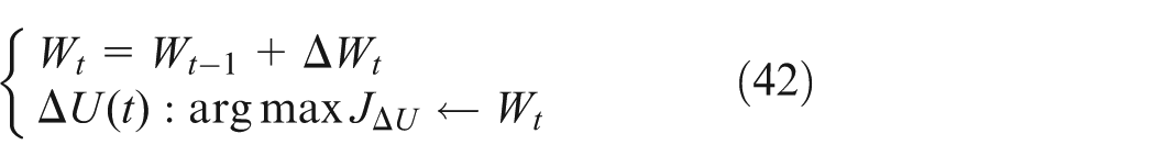
1. Determine the optimal weight matrix $[Q_{y_e},Q_{{\phi }_e},Q_{v_e},R]$ based on vehicle status and reference trajectory.

2. According to a fixed weight matrix, the quadratic programming problem is solved.

Based on the DQN algorithm, the adaptive adjustment of the weight matrix of MPC is achieved. At each calculation time step, the current optimal value is given, and the online update of the Q network is synchronously completed.

The specific steps of the adaptive adjustment method for the weights of MPC based on DQN are as follows:

• Step 1: The tracked unmanned vehicle is regarded as an agent, and the external conditions of the tracked vehicle and some body characteristics (such as track material, mechanical structure, etc.) are regarded as environment. The action space, the state space, the state-transition equation and the reward function in the DQN algorithm are defined.

• 1. State space

The state of the tracked unmanned vehicle at time t is defined, including the current lateral deviation, heading angle deviation, speed error, and the original weight matrix:

$$s_t=[y_e(t),{\phi }_e(t),v_e(t),W_{t-1}]$$

(39)

• 2. Action space

The actions within each time step are adjustments to the weight, therefore the action space is defined as:

$$a_t=\Delta W_t=[\Delta Q_{y_e}(t),\Delta Q_{{\phi }_e}(t),\Delta Q_{v_e}(t),\Delta R(t)]$$

(40)

Where $\Delta Q_{y_e}(t),\Delta Q_{{\phi }_e}(t),\Delta Q_{v_e}(t),\Delta R(t)$ corresponds to the variation of the four weight coefficients of the objective function. In order to improve the efficiency of training and ensure the stability of vehicle driving when using the weight matrix for control, each adjustment of the weight should not be too large. Therefore, it is considered to reduce the dimension of the action space, so that $\Delta Q_{y_e}(t)$ $\Delta Q_{{\phi }_e}(t)$ $\Delta Q_{v_e}(t)$ and $\Delta R(t)$ are both valued in $[-0.1,0,+0.1]$ . Therefore, for each state space, there are $\mathrm{nu}{m}_a=3^4=81$ adjustment actions corresponding to it. Based on the ε Greedy algorithm, the next action is selected as followed:

$$\pi (a|s)=\{\begin{array}{c}\epsilon ,a\ne \arg max{Q}_{\varphi }(s,a),\hfill \\ \multicolumn{1}{c}{1-\epsilon ,a=\arg max{Q}_{\varphi }(s,a)}\end{array}$$

(41)

Among them, $\pi (a|s)$ has a probability of ε for random “exploration” in the s state, and a probability of $1-\epsilon$ to output the action with the highest Q value based on the current Q network.

• 3. State-transition equation

As an action $a_t=\Delta W_t=[\Delta Q_{y_e}(t),\Delta Q_{{\phi }_e}(t),\Delta Q_{v_e}(t),\Delta R(t)]$ is selected, which means that the weight has been adjusted, and the determined target weight is used for the quadratic programming solution as followed:

$$\{\begin{array}{c}{W}_t=W_{t-1}+\Delta W_t\hfill \\ \multicolumn{1}{c}{\Delta U(t):\arg max{J}_{\Delta U}\leftarrow W_t}\end{array}$$

(42)

Subsequently, the optimal motor driving torque is obtained and applied on the tracked unmanned vehicle, causing a transition in the transition space as followed:

$$\{\begin{array}{c}[T_R,T_L]=u(t)=u(t-1)+\Delta U(t)\hfill \\ \multicolumn{1}{c}{s_{t+1}=f_{\mathrm{real}}(s_t,u(t))}\end{array}$$

(43)

where f _real represents the feedback state of the actual tracked unmanned vehicle under the given driving torque.

• 4. Reward function

The ultimate goal of weight adaptive adjustment is to achieve optimal tracking accuracy, so a negative root mean square error is designed as a reward:

$$r_t=-\sqrt{y_e^2+{\phi }_e^2}$$

(44)

• Step 2: Set up the Q network and target Q network architecture. The two network architectures are the same, except that the update frequency of internal parameters is different. The hidden layer of Q network is designed as a feedforward neural network consisting of two full connection layers. The number of units is 16 and 8, respectively. The activation function uses the ReLU function. Where, the input layer dimension is determined to be 7 based on s, and the output layer dimension is 1. Assuming that the network parameter of the Q network at time t is Q _t and the network parameter of the target Q network is $Q_t^{\prime }$ . Its value is initialized.

• Step 3: Establish a state buffer $\mathrm{set}\left\{\mathrm{transition}\right\}=\left\{[s_t,a_t,r_t,s_{t+1}]\right\}$ and randomly extract a training dataset to train and update the Q network parameters.

The Q value under Q network is defined as $Q(s,a|\theta )$ , and the gradient descent method is used to update the parameters of Q network.

$${\theta }_{t+1}={\theta }_t-\alpha {\nabla }_{{\theta }_t}L({\theta }_t)$$

(45)

Where, α is the learning rate, and controls the size of each parameter update. Usually, we use a smaller α (such as 10⁻⁴ or 10⁻⁵), and gradually reduce α during the training process to balance the contradiction between the learning speed and the stability requirements. ${\nabla }_{{\theta }_t}L({\theta }_t)$ is the gradient of the loss function $L({\theta }_t)$ relative to parameter θ _i at time t, and the loss function can be defined as the mean squared error of Q value of the prediction network and the target network according to the equation (44):

$$\begin{array}{c}\multicolumn{1}{c}{L({\theta }_t)=}\\ \multicolumn{1}{c}{E\left[{(r_t+\gamma {max}_{a_{t+1}}Q(s_{t+1},a_{t+1}|{\theta }_t^{\prime })-Q(s_t,a_t|{\theta }_t))}^2\right]}\end{array}$$

(46)

The above steps have completed the update of the Q network at time t. After each k time steps, the target Q network is updated once as followed:

$$\theta \prime =\theta$$

(47)

The pseudocode of the algorithm for adaptive adjustment of MPC weights based on DQN is shown in Algorithm 1.

Algorithm 1. MPC weight adaptive adjustment algorithm based on DQN
Input: state space S, action space A, discount rate γ, Learning rate α, update target network steps k, exploration rate ε
1: Initialize the experience playback area M and set the capacity to N
2: Initialize Q network parameters θ
3: Synchronize target Q network parameters ${\theta }^{\prime }=\theta$
4: for episode=1:m:
5: Initialization status $s=[y_e,{\phi }_e,v_e,W]$
6: for time = 1: n
7:  Select action a in state s
8:   Adjust the original weights: $W^{\prime }=W+\Delta W{|}_a$ . The MPC controller uses weight W t to solve the torque output to the tracked unmanned vehicle and senses changes in state variables, collecting relevant information
9:   Calculate the reward value
10:   Obtain new environmental status s′
11:   Store status transfer information $(s,a,r,s\prime )$ in M
12:   Collect $(s,a,r,s\prime )$ from M
13:    $y=\{\begin{array}{c}r,\mathrm{if}{s}^{\prime }is\mathrm{th}e\mathrm{en}dof\mathrm{the}\mathrm{sequence}\hfill \\ \multicolumn{1}{c}{r+\gamma {max}_{a\prime }{Q}_{\theta \prime }(s\prime ,a\prime ),\mathrm{ortherwise}}\end{array}$ .
14:   Training Q network with Loss function $(y-Q_{\theta }(s,a))$
15:   Update target Q network parameters ${\theta }^{\prime }\leftarrow \theta$ every k steps
17:  end
18: end
Output: MPC optimal weight adaptive adjustment strategy

Simulation and experiment

MATLAB/Simulink–RecurDyn joint simulation

This dual motor driven tracked vehicle is a typical multivariable and nonlinear system, and a numerical analytical mathematical model is difficult to describe the actual dynamics behavior of the vehicle. RecurDyn multi-body simulation software is used to establish a 3D virtual model of the tracked vehicle and a road surface model. The dual motor driven tracked vehicle model in RecurDyn is shown in the Figure 8. The dynamics parameters of the tracked vehicle are shown in Table 1. The trajectory tracking control strategy model shown in the figure is built in MATLAB/Simulink. Through collaborative simulation using RecurDyn and MATLAB/Simulink, the trajectory tracking control considering actual vehicle dynamics and operational behavior is achieved, as shown in Figure 9. The inputs of the RecurDyn module are the torques of the active wheels on both sides, and the outputs include the speeds of the active wheels, the vehicle speed, the trajectory of vehicle center, the yaw rate, the longitudinal speed of the track, etc.

Figure 8.

The tracked vehicle model in RecurDyn.

Table 1.

Dynamic model parameters of tracked vehicle dynamics based on RecurDyn.

Components	Number	Moment of inertia (kg/m)	Stiffness	Damping coefficient
Capstan	2	279,379	18,000	10
Road wheel	10	685,898	12,000	10
Towing wheel	6	5121	15,000	10
Track shoe	3.51989	1989	9000	10

Figure 9.

MATLAB/Simulink–RecurDyn joint simulation platform.

Simulation results

In order to verify the advantages of the proposed trajectory tracking control strategy based on the dynamics prediction model compared with the traditional control strategy based on kinematics in terms of control accuracy and stability, a double lane trajectory tracking test is designed under the conditions of vehicle speeds of $18\mathrm{and}36\mathrm{km}/\mathrm{h}$ , respectively, and high road adhesion coefficient μ=0.85 (Figure 10). To verify the effectiveness of the proposed DQN based weight adaptive adjustment method, a tracking condition was designed at $v=36\mathrm{km}/h$ .

• 1. ν=18km/h, μ=0.85

The screenshot of the visualized trajectory dynamic tracking simulation in RecurDyn is shown in Figure 11, and the simulation results of double shift lane tracking are shown in Figure 12.

Figure 10.

Screenshot of MPC trajectory tracking visualization simulation based on dynamics prediction model, $v=18\mathrm{km}/h$ .

Figure 11.

Screenshot of the MPC trajectory tracking visualization simulation based on dynamics prediction model, $v=36\mathrm{km}/h$ .

Figure 12.

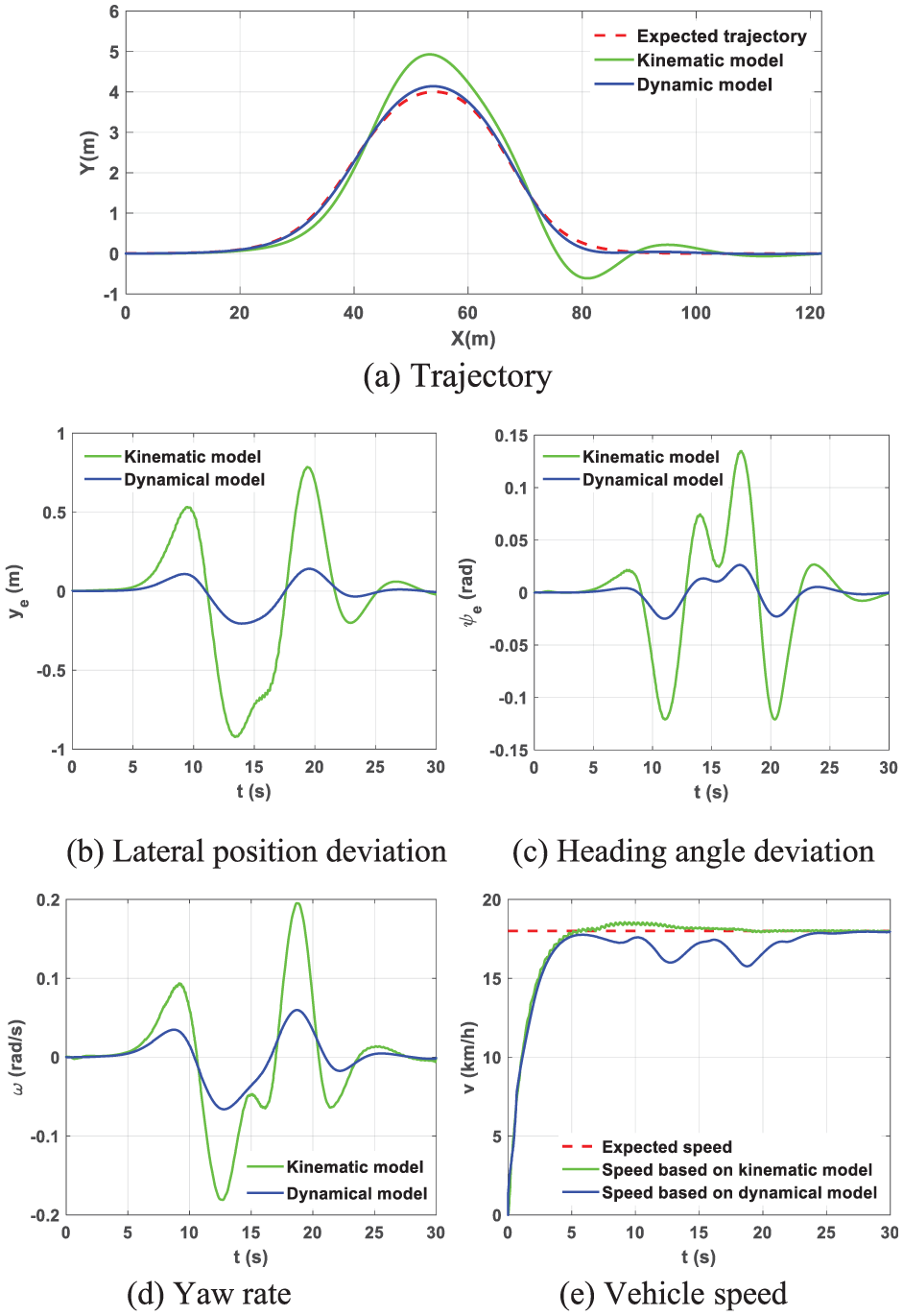
Comparison of simulation results of the MPC control based on kinematics/dynamics prediction model at $v=36\mathrm{km}/h$ : (a) trajectory, (b) lateral position deviation, (c) heading angle deviation, (d) yaw rate and (e) vehicle speed.

From Figure 13(a) to (c), it can be seen that there is a significant lateral deviation and heading angle deviation when the tracked vehicle turns and changes lanes at times of t= 9.5s, t= 13.5s, and t= 20s. The maximum lateral deviation of the MPC control strategy based on kinematics prediction model is 0.89m, and the maximum heading angle deviation is 0.13rad. The maximum lateral deviation of the control strategy based on the dynamics prediction model is 0.21m, and the maximum heading angle deviation is $0.02\mathrm{rad}$ . Compared with the conventional benchmark kinematic MPC controller, the maximum lateral deviation and heading angle deviation of the MPC using the proposed dynamics prediction model are reduced by 76.4% and 84.6%, respectively. This proves that tracked vehicles using the proposed MPC tracking control strategy have better tracking performance during low-speed steering.

Figure 13.

Comparison of simulation results of the MPC control based on kinematics/dynamics prediction model at $v=18\mathrm{km}/\mathrm{h}$ : (a) trajectory, (b) lateral position deviation, (c) heading angle deviation, (d) yaw rate and (e) vehicle speed.

Figure 13(d) shows that the control strategy based on the dynamics prediction model has a smaller yaw rate, and the controlled tracked unmanned vehicle turns more smoothly.

From Figure 13(e), it can be seen that due to the use of lateral and longitudinal decoupling methods in the kinematics control strategy, the deviation between the output speed and the expected vehicle speed is relatively small. The dynamics based MPC control strategy considers lateral and longitudinal coupling. When the lateral deviation and heading angle deviation are large, multi-objective optimization is used to balance and adjust the longitudinal speed in real time. Therefore, the longitudinal speed will be slightly reduced when the vehicle turns.

• 2. $v=36\mathrm{km}/h,\mu =0.85$

The screenshot of the visualized trajectory dynamic tracking simulation in RecurDyn is shown in Figure 11, and the simulation results of double shift lane tracking are shown in Figure 12.

From Figure 12(a) to (c), it can be seen that there is a significant lateral deviation and heading angle deviation when the tracked vehicle turns and changes lanes at times $t=5.2\mathrm{s}$ , $t=9.3\mathrm{s}$ , and $t=13\mathrm{s}$ . The maximum lateral deviation of the MPC control strategy based on kinematics prediction model is $2.5\mathrm{m}$ , and the maximum heading angle deviation is $0.26\mathrm{rad}$ . The maximum lateral deviation of the control strategy based on the dynamics prediction model is $1.04\mathrm{m}$ , and the maximum heading angle deviation is $0.21\mathrm{rad}$ . Although the lateral deviation and heading angle deviation increase at v = 36 km/h, compared with the conventional benchmark kinematic MPC controller, the maximum lateral deviation and heading angle deviation of the MPC using the proposed dynamics prediction model are reduced by 58.4% and 18.6%, respectively. This proves that the MPC trajectory tracking control strategy based on the dynamics prediction model can effectively improve the trajectory tracking accuracy in the middle and low speed steering process.

As shown in Figure 12(d), the yaw rate of the trajectory tracking strategy based on the kinematics prediction model exceeds the limit of $0.2\mathrm{rad}/\mathrm{s}$ up to $0.33\mathrm{rad}/\mathrm{s}$ , resulting in a decrease in driving smoothness. Due to the consideration of dynamics factors in MPC trajectory tracking control based on dynamics models, the steering becomes smoother.

As shown in Figure 12(e), the proposed MPC trajectory tracking control strategy based on the dynamics prediction model can ensure tracking accuracy by appropriately adjusting the vehicle speed through multi-objective optimization algorithms.

• 2. Adaptive weight adjustment based on DQN: $v=36\mathrm{km}/\mathrm{h},\mu =0.85$

In order to validate the proposed DQN based MPC weight adaptive adjustment method, under the expected vehicle speed of $v=36\mathrm{km}/\mathrm{h}$ and high road adhesion $\mu =0.85$ conditions, a trajectory tracking control strategy based on the dynamics model is used to repeat double lane trajectory tracking experiments, in order to achieve the goal of training the DQN network. In theory, as the number of experiments increases, the parameters of the DQN network gradually tend to be optimal and converge. Hyperparameters are shown in Table 1 and convergence curves are shown in Figure 14. The tracking results of using the weight matrix of empirical method and adaptive adjustment weights with Episode of 10 and 1000 are shown in Figure 15.

Figure 14.

Convergence curves.

Figure 15.

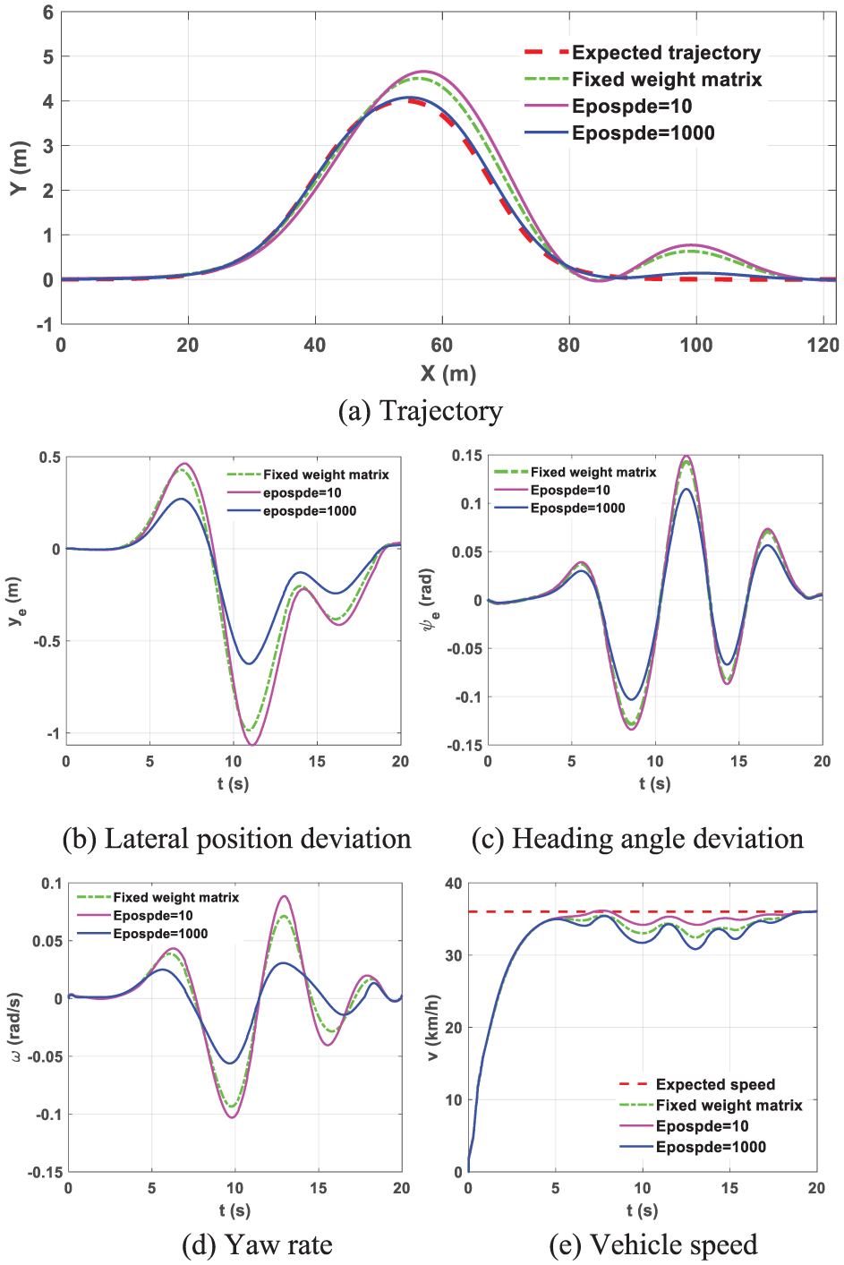
Comparison of the MPC trajectory tracking results of dynamics prediction models with fixed weight and adaptive weight adjustment: (a) trajectory, (b) lateral position deviation, (c) heading angle deviation, (d) yaw rate and (e) vehicle speed.

As shown in the Figure 14, the Average Loss decreases rapidly in the initial phase and stabilizes at a minimal value after ∼400 episodes, indicating that the prediction error is minimized. Concurrently, the average total reward rises steadily and converges to a stable value of around 800 after 750 episodes. These synchronous trends confirm that the DQN agent has effectively learned the optimal weight adjustment strategy without divergence.

From Figure 15, when Episode = 10, the tracking effect is even worse than the empirical method. However, with the increase of training rounds, the tracking effect is significantly improved. From Figure 15(b) to (e), it can be seen that when the number of Episode is 1000, the maximum lateral deviation and heading angle deviation further decrease by 36.6% and 19.7%.

Experimental results

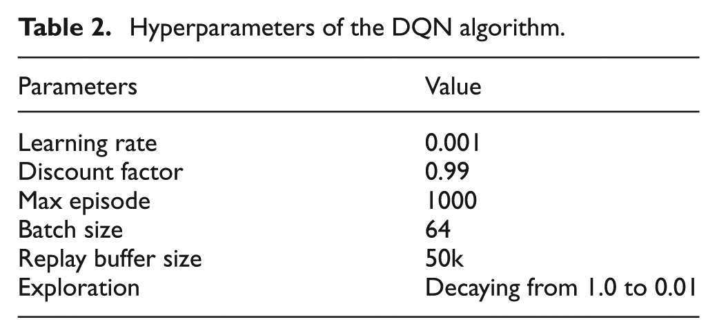
A dual motor driven tracked unmanned vehicle was built on the actual vehicle as shown in Figure 16, with specific parameters shown in Table 2, to further verify the control effect and real-time performance of the proposed trajectory tracking control strategy based on dynamics prediction model on the actual vehicle (Table 3).

Figure 16.

A real vehicle platform for the dual motor driven tracked vehicle.

Table 2.

Hyperparameters of the DQN algorithm.

Parameters	Value
Learning rate	0.001
Discount factor	0.99
Max episode	1000
Batch size	64
Replay buffer size	50k
Exploration	Decaying from 1.0 to 0.01

Table 3.

Tracked unmanned vehicle parameters.

Parameters	Numerical value
Track gauge, B/mm	1300
Number of rounds, 2n	10
Driving wheel radius, $r_z/\mathrm{mm}$	150
Track grounding length, L/m	1.7
Rolling resistance coefficient, f	0.04
Maximum steering drag coefficient, ${\mu }_{max}$	1
Gear ratio, i	6.35
Vehicle mass, m/kg	120
Mass increase coefficient, δ	1.5
Moment of inertia, $J/\mathrm{kg}/m^2$	300

Due to safety restrictions on the actual site, v = 10.8 km/h, the experimental results are shown in Figure 17, and the on-site diagram is shown in Figure 18.

Figure 17.

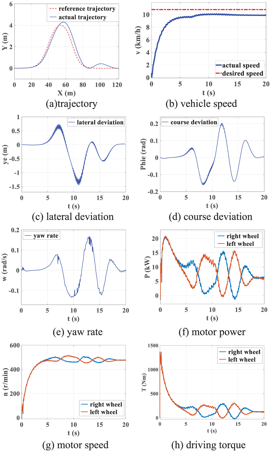
Experimental results of trajectory tracking for the tracked unmanned vehicle: (a) trajectory, (b) vehicle speed, (c) lateral deviation, (d) course deviation, (e) yaw rate, (f) motor power, (g) motor speed and (h) driving torque.

Figure 18.

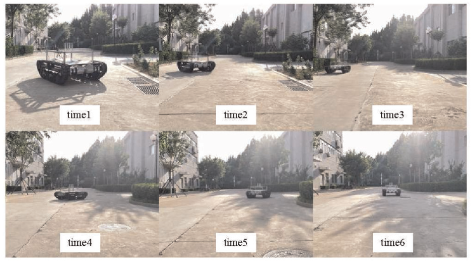
Experimental site of trajectory tracking for the tracked unmanned vehicle.

Due to the limitations of the experimental site and to ensure the safety of the actual vehicle experiment, the trajectory tracking performance of unmanned tracked vehicles under dual lane shifting conditions was only verified under low speed driving conditions. The tracked vehicle was set to an expected speed of 10.8 km/h, and the experimental results are shown in Figure 17. The experimental photos are shown in Figure 18. From the Figure 17(a) and (b), it can be seen that the unmanned tracked vehicle using the proposed NMPC of dynamics prediction models has good trajectory and speed tracking accuracy.

Conclusion

1. Aiming at the problem of poor tracking accuracy caused by the coupling of longitudinal and lateral dynamics in traditional MPC trajectory tracking control strategies based on kinematics prediction models, a MPC trajectory tracking strategy that integrates kinematics and dynamics models is proposed, achieving a integrated control of the trajectory tracking and handing stability based on yaw rate control. The maximum lateral deviation and heading angle deviation were reduced by 58.4% and 18.6%.

2. The weight matrix of the objective function in traditional MPC controllers is constant. However, with the continuous changes of measurable disturbances such as reference trajectories and unmeasurable disturbances such as external environments, an unchanged weight matrix of the objective function cannot guarantee the optimal control performance throughout the entire working process. A weight matrix adaptive adjustment method based on deep Q-network (DQN) reinforcement learning strategy is proposed for solving the optimal control torque using MPC, which further reduced the maximum lateral deviation and heading angle deviation by 36.6% and 19.7%.