Sage Journals: Discover world-class research

Abstract

This paper focuses on the challenge of predicting the components and full-engine reliability of automotive diesel engines and proposes an integrated approach combining mechanistic modeling with statistical data. The mechanism model was developed for engine performance, dynamics, as well as wear and fatigue damage of critical components. Uncertain parameters were processed using Monte Carlo and Latin hypercube sampling methods to compute damage distributions and reliability curves for both components and full-engine system. Using a specific automotive diesel engine as a case study, the wear model of the main bearing shell was verified on the reliability test bench, with an error of only 2.03%. Damage calculations were conducted on several critical components, the results demonstrate that damage to the components conforms to the cumulative damage phenomenon, moreover, the damage distribution for the piston ring and exhaust valve exhibits an increasing dispersion under the effects of stochastic influences. The reliability curves align with the bathtub curve. The mechanism model yields a full-engine MTBF of 7091 h (242,000 km), a B10 life of 6050 h (206,000 km), and a system-wide MTBF of 1490 h (50,000 km) after integrating subsystem failure rates. This methodology offers effective tools for engine reliability design and predictive maintenance.

Keywords

diesel engine MTBF lifetime prediction reliability analysis mechanism model

Introduction

Among modern land transportation modes, automobiles occupy a dominant position in terms of the number of vehicles in operation, penetration rate, operational scope, and the volume of passenger and freight turnover. Diesel engines are widely employed in commercial vehicles, including buses and trucks, owing to their advantages such as high-power output and superior fuel economy. In recent years, with the upgrading and high-quality development of the automotive industry, the reliability and service life of diesel engines have garnered increasing attention.

In the field of engine reliability research, the methods of establishing mechanism models and data-driven approaches have been widely employed.

Data-driven methods play a critical role in lifespan prediction, leveraging historical data to extract failure modes or predict degradation trends—for instance, assessing product reliability through extensive failure rate data. Tang et al.¹ utilized experimental data and machine learning techniques to predict the fatigue life of cold-expanded hole structures, validating the effectiveness and robustness of their approach. Wang and Zhang² conducted a reliability analysis of a heavy-duty truck diesel engine based on subsystem failure ratios derived from after-sales maintenance data. Xie et al.³ performed a stochastic process-based, data-driven degradation analysis using degradation data from a specific aero-engine.

Methods based on machine learning and neural networks have gained popularity. Ma and Yuan⁴ integrated an Improved Golden Jackal Optimization algorithm with a long-short-term memory neural network to enhance the prediction accuracy of remaining useful life for equipment. Warter et al.⁵ proposed a data-driven prediction method for key combustion parameters in intelligent diesel fuel injectors, offer a new solution for condition monitoring and performance optimization in large engine applications.

Mechanism models also play an essential role in diesel engine reliability analysis. These models typically rely on physical or chemical principles and employ precise parametric descriptions to predict system performance, failure evolution patterns, and lifespan. Essentially, such approaches analyze engine behavior by constructing mathematical models that reflect internal working principles and logical relationships. Wei et al.⁶ established a mathematical model linking cylinder pressure and diesel engine lifespan based on the ideal gas law, enabling personalized lifespan prediction. Zhang et al.⁷ investigated the fracture mechanism of threaded holes in diesel engine main bearings and identified operational loads as the primary cause of failure. Cui et al.⁸ applied fundamental tribologic theories of automotive engines to analyze the causes and patterns of cylinder liner wear. Liu et al.⁹ studied engine pistons by calculating thermal loads, mechanical loads, and stresses under thermo-mechanical coupling conditions. Yin et al.¹⁰ proposed a new life-cycle multi-physics model to coupling the evolution of bearing wear. Wang et al.¹¹ developed a high-precision wear model for predicting the wear volume of piston–cylinder pair. Dowell et al.¹² developed a real-time model simulating engine cylinders and combustion processes. Ivana et al.¹³ integrated the logical framework of fault tree analysis with Bayesian networks to study failure modes and mechanisms in diesel engine subsystems.

With continuous technological advancements, the use of simulation tools to construct physics-based models for reliability analysis has become increasingly widespread. For example, Zhang et al.¹⁴ employed ANSYS to conduct a comprehensive analysis of the three-dimensional temperature field and stress-strain distribution in a diesel engine piston, evaluating its lifespan and structural safety. Zhu et al.¹⁵ applied the finite element method to analyze a diesel engine crankshaft model and its sub-models. Wang et al.¹⁶ developed a finite element model to simulate the evolution of wear depth on the piston skirt contact surface under actual engine conditions. Service life under frequent wear was estimated by monitoring pre-load loss in the crown-skirt connecting bolts.

However, engines consist of numerous highly complex components, and achieving higher modeling accuracy has made it difficult for purely physics-based or purely data-driven methods to fully meet predictive requirements. As a result, hybrid models that integrate both approaches have attracted growing attention. Cao et al.¹⁷ proposed a hybrid data-driven and model-driven learning framework for remaining useful life (RUL) prediction to overcome the limitations of individual approaches. Pulpeiro¹⁸ combined data-driven methods to characterize the performance of the turbocharger and intake manifold with physics-based models for other relatively simpler components, achieving high-precision prediction of gas exchange processes in diesel engines. Xiao et al.¹⁹ proposed a method that integrates an independent recurrent neural network with physical knowledge of the engine, establishing a full engine model that significantly improved the accuracy and reliability of performance predictions. Lang et al.²⁰ introduced an approach combining physical and data-driven models to enhance the numerical simulation accuracy of medium-speed diesel engines, particularly under transient conditions. By optimizing the matching between the turbocharger and the engine, the method improved the prediction of pressure dynamics and nitrogen oxide emissions.

In aero-engine reliability research, comprehensive databases are readily available to support analysis. However, automotive engines lack sufficient data samples, as prolonged durability tests—such as those lasting 10,000–20,000 h—are often impractical for accumulating failure data. While simulation tools like ANSYS are effective for 3D modeling of individual components, such as wear and structural analysis, they encounter limitations when applied to full-engine systems due to modeling complexity and computational demands. The intricate structure and failure mechanisms of engines also constrain purely physics-based modeling approaches. Therefore, integrating reliability data statistics with mechanistic modeling presents a promising direction for advancing whole-engine reliability studies and uncovering deeper systemic insights.

This study conducts reliability analysis on several critical components of automotive diesel engines, including cylinder liners, piston rings, crankshafts, and main bearing shells. These components are manufactured by original engine producers, and their structural data are available. Given their well-understood failure mechanisms, reliability analysis can be effectively performed using physics-based models. In contrast, sealing fasteners such as bolts and cylinder gaskets are typically sourced from external suppliers, and detailed modeling data are often unavailable. Therefore, mathematical statistical methods are employed for their reliability assessment.

Reliability is the core metric for evaluating engine durability, defined as the probability that a product performs its intended function without failure under stated conditions for a specified period of time.²¹ The reliability prediction model proposed in this study integrates both statistical data and mechanism model to evaluate and predict the reliability of the engine as a whole. As shown in Table 1, this approach is compared with earlier methods in terms of advantages and limitations.

Table 1.

Comparison of the proposed method and earlier methods.

Metric	Integrated method	Mechanism models	Statistical data
Reliability prediction accuracy	High (integrates mechanisms and statistics)	High (mechanism simulation)	Moderate (limited to input data trends)
Inputs required	Moderate (statistical data and mechanism)	High (full mechanism subsystems)	Low (focused on historical data)
Computational effort	Moderate (supports Monte Carlo simulation)	High (dependent on full system models)	Low (limited calculation effort)
Coupled simulation capability	Yes (support integration of subsystems)	Partial (computationally expensive)	No (does not support integration)

Graphical modeling is adopted to significantly streamline the modeling process, wherein a straightforward graphical modeling tool has been developed to represent engine components as icons and energy transfers between them as connecting lines. Unlike traditional methods that rely on computationally intensive 3D engine models and require deep expertise in simulation software, this approach enables a more intuitive and vivid examination of engine reliability. By allowing practitioners to intuitively model energy flows between components, the tool reduces the temporal and cognitive complexity of reliability analysis without compromising accuracy.

Methods

To address the reliability analysis challenges of the engine and its components, this paper proposes a method that integrates the mechanism model and the data statistics model. The reliability prediction workflow is shown in Figure 1. The mechanism model consists of three core components: a performance computing model, a dynamic computing model, and a damage computing model. The performance computing model simulates a full engine cycle to obtain parameters such as cylinder temperature, fuel consumption and brake mean effective pressure as functions of crankshaft angle. The dynamic computing model then uses these results to determine the time-varying loads acting on each component, also expressed with respect to crankshaft rotation. Based on these boundary conditions, the damage computing model predicts wear and fatigue parameters for critical components including the cylinder liners and piston rings. The mechanism model also accounts for performance degradation caused by wear and gas leakage between the cylinder liner and piston ring. To incorporate uncertainties from operating conditions, assembly tolerances, and material properties, Monte Carlo and Latin hypercube sampling methods are employed to generate input samples. Through multiple simulations with these samples, the model produces a time-dependent distribution of damage for each component. The statistical model includes parameters such as the failure rates of external factory components and other engine subsystems with existing data. Finally, following reliability theory, the probabilistic damage distributions from the mechanistic simulations are combined with prior statistical data to evaluate the time-varying reliability of both the full-engine and its critical components.

Figure 1.

The reliability modeling process integrating mechanism and data statistics.

Performance computing and dynamic computing model of the engine

The performance computing model integrates four key subsystems: the intake and exhaust manifolds, the intercooler, the cylinders, and the turbocharger system. The energy transfer between these subsystems is described through mathematical modeling frameworks.²² In the process of subsystem modeling, models with a 0D/1D resolution are typically employed.^23–26 For the intake and exhaust manifold subsystems, the 0D volumetric method is adopted, where the intake and exhaust pipe, and cylinder are discretized into multiple uniform volumes. In this research, the intercooler is not the primary focus of analysis. Therefore, a simple 1D thermodynamic model is utilized for it. Regarding the turbocharger system, the MAP diagram model is applied. Essentially, this is a 0D model, that is, based on a 2D data table, provides the overall performance relationship between the inlet and outlet, offers a balance between predictive accuracy and computational cost. Within the cylinder subsystem, the combustion model makes use of a 0D resolution dual Wiebe model and the heat transfer model employs the Woschni formula, to efficiently compute global average combustion parameters. Gas leakage, which contributes to performance degradation, is accounted for via a 1D isentropic flow formulation to estimate the leakage mass flow rate. As wear occurs between the cylinder liner and piston rings during engine operation, the clearance volume increases, resulting in combustion gas leakage. This leakage subsequently leads to a reduction in mechanical efficiency. Therefore, the performance computing model incorporates the effect of such degradation to accurately reflect the engine’s operational behavior over time.^27,28

The dynamic computing model utilizes parameters derived from the performance computing model—such as brake mean effective pressure, cylinder temperature, and fuel consumption—to compute the load and temperature conditions of critical structural components. These include the cylinder liners, piston rings, crankshafts, and the connecting rod big bearing shells, through kinematic and dynamic analysis of the crankshaft-connecting rod mechanism. The resulting values serve as boundary conditions for subsequent mechanistic modeling.

Mechanism model of critical components

Damage to components primarily manifests in two forms: wear and fatigue. Wear calculation is commonly performed using the Archard wear formula.²⁹ According to Archard, wear results from the adhesion and fracture of micro-scale asperities on contact surfaces during sliding, leading to material detachment in the form of fine particles. The depth of wear is influenced by the actual contact stress, material properties, and sliding distance. The depth of wear, denoted as h, is given by the following formula:

h = K \frac{P_{c}}{H} S,

(1)

where K is the dimensionless wear coefficient of the material, H is the Brinell hardness of the material, P_c is the contact pressure, S is the relative sliding distance.

For the cylinder liner-piston ring friction pair, the contact pressure varies with the crankshaft rotation angle and is determined by factors such as the instantaneous gas pressure, piston ring elastic force, and ring groove friction force. Similarly, the load on the connecting rod big bearing and the main bearing also varies with the crankshaft rotation angle. Once the loads acting on each friction pair are obtained, the depth of wear can be calculated according to the wear formula.

For components such as pistons, crankshafts, connecting rods and bolts, which are primarily subject to fatigue damage, it is necessary to calculate the alternating stress at critical failure locations based on the theory of fatigue damage accumulation. The alternating stress in pistons can generally be determined using the finite element method³⁰ and may be represented through a logarithmic formulation of the generalized Eyring model³¹ as follows:

\ln (N) = a + b \cdot f (s_{1}) + c \cdot f (s_{2}) + d \cdot f (s_{1}) (s_{2}),

(2)

where N is the fatigue life, $f (s_{1})$ is the mechanical stress term, $f (s_{2})$ is the thermal stress term, $a, b, c$ , and d are constants determined through finite element calculations.

The alternating stress of the crankshaft is calculated according to the formula provided in the diesel engine design manual.³² The stress amplitude σ₋₁ under symmetric loading is then determined using the modified Goodman formula³³ as follows:

\frac{σ_{a}}{σ_{- 1}} + \frac{σ_{m}}{σ_{b}} = 1,

(3)

where σ_b is the ultimate tensile strength of the material, σ_m and σ_a represent the mean stress and stress amplitude under actual operating conditions, respectively, σ₋₁ is the fully reversed stress amplitude (i.e. at a stress ratio of $R = - 1$ ). Finally, the fatigue life N of the crankshaft is determined using equation (4),³⁴ based on the material $S - N$ curve:

lgN = k_{1} + k_{2} \lg σ_{- 1},

(4)

where N is the fatigue life, k₁ and k₂ are material constants derived from fitting the $S - N$ curve.

Statistical model of critical components

In engines, sealing elements and fasteners including bolts and gaskets are typically sourced from external suppliers. Such standardized commercial parts often have substantial statistical reliability data available in the market, including failure rates. The failure rate of the seal can be modeled as follows³⁵:

λ_{SE} = λ_{SE, B} [\frac{K_{1} (P_{1}^{2} - P_{2}^{2}) L G^{3}}{Q_{f} v_{a} w P_{2}}],

(5)

where λ_SE denotes the failure rate of the gasket or seal under operational environmental conditions, λ_SE,B is the baseline failure rate, K₁ is an empirical constant, P₁ and P₂ are the upstream and downstream pressure, respectively, L is the contact length, G is the conductivity parameter, Q_f is the allowable leakage rate under service conditions, v_a is the absolute fluid viscosity, w is the width of the seal. Among these, G can be expressed as:

G = 0.23 {(\frac{M}{C})}^{\frac{3}{2}} \cdot {R_{a}}^{\frac{2}{3}},

(6)

where M is the Young’s modulus of rubber or elastic materials, C is the contact stress, R_a is the surface roughness.

According to equation (5), the failure rates of seals under various operational conditions can be computed. Once the failure rate is obtained, the corresponding exponential failure probability density function³⁶ can be expressed as follows:

f (t) = λ (t) e^{- λ (t)},

(7)

where $λ (t)$ is the instantaneous failure rate at time t.

Integrated mechanistic–statistical modeling

The damage predicted by the mechanism model is denoted as $D_{M} (t)$ , while that derived from statistical data is denoted as $D_{S} (t)$ . Both are time-varying random vectors. The time-dependent reliability of the full-engine system can be expressed as:

\begin{matrix} R (t) = R {d_{m} (t) < 1, d_{s} (t) < 1} \\ = R {d_{m} (t) < 1} R {d_{s} (t) < 1 | d_{m} (t) < 1}, \end{matrix}

(8)

where $d_{m} (t)$ and $d_{s} (t)$ represent certain norms of the damage vectors $D_{M} (t)$ and $D_{S} (t)$ , respectively, and are expressed as follows:

d_{m} (t) = \begin{matrix} ∥ D_{M} (t) ∥ \end{matrix};

(9)

d_{s} (t) = \begin{matrix} ∥ D_{S} (t) ∥ \end{matrix} .

(10)

The mechanism model evaluates reliability $R {d_{m} (t) < 1}$ through the following process:

The Monte Carlo method is employed to convert random variables—including operating conditions, assembly tolerances, and material properties—into statistical sample data.

For each simulated case, parameters including performance, dynamics, wear rate, and fatigue damage were computed to generate time-dependent damage samples $D_{M} (t)$ of critical components under various failure modes.

The sampled value of the full-engine damage $d_{e} (t)$ is denoted as $d_{e}^{i} (t) = \overset{k}{\max_{j = 1}} {D_{M}^{ij} (t)}$ , $i = 1, 2, 3, \dots, n$ , where n is the number of samples, j indexes the j-th component analyzed by the mechanism model, and k is the total number of components considered in the model.

The reliability of each component is computed by formula $R {d_{m}^{j} (t) < 1} = \frac{count (D_{M}^{ij} (t) < 1)}{n}$ .

The reliability of the full-engine system of mechanism model is computed by formula $R {d_{m} (t) < 1} = \min_{j = 1, 2, 3, \dots} {R {d_{m}^{j} (t) < 1}}$ .

The reliability of the component whose failure rate is computed based on statistical data is expressed as:

\begin{matrix} R {d_{s} (t) < 1 | d_{m} (t) < 1} = R {d_{s} (t) < 1} \\ = \underset{a}{Π} R {D_{S}^{a} (t) < 1}; \end{matrix}

(11)

R {D_{S}^{a} (t) < 1} = 1 - \int_{0}^{t} λ_{a} (η) e^{- \int_{0}^{η} λ_{a} (ξ) d ξ} d η,

(12)

where a indexes the ath component analyzed using statistical data, $D_{S}^{a} (t)$ indexes the damage matrix of the ath component at time t, derived from statistical data, $λ_{a} (η)$ indexes the instantaneous failure rate of the ath component at time η. The full-engine reliability of the machine at time t is expressed as:

R (t) = \min_{j = 1, 2, 3, \dots} {R {d_{m}^{j} (t) < 1}} \underset{a}{Π} R {D_{S}^{a} (t) < 1},

(13)

in the formula, the value $d_{m} (t)$ , derived from the mechanism model, incorporates interactions between components and the full-engine, mutual influences among components, as well as couplings between different failure modes within the same component. This comprehensive integration significantly enhances the confidence level of the reliability assessment.

Based on the reliability formula R(t), the service life τ corresponding to a specified reliability level can be determined as follows³⁷:

τ = \int_{0}^{+ \infty} R (t) dt,

(14)

for a repairable engine system, this corresponds to the mean time between failures (MTBF).

Sample generation using the Monte Carlo simulation and Latin hypercube sampling

The Monte Carlo simulation (MCS) method demonstrates significant advantages in addressing complex physical systems. The procedure begins with the construction of a mechanical mathematical model, followed by the generation and simulation of random samples that conform to specified probability distributions. Subsequently, statistical analysis is performed on the simulation outcomes to estimate system characteristics. However, when using simple random sampling, the convergence rate of the statistical error in estimating these characteristics is $O (1 / \sqrt{N})$ , implying that reducing the error by a factor of two requires quadrupling the sample size, thereby substantially increasing computational costs.

To improve computational efficiency and better capture critical regions of the parameter space—particularly those associated with rare events such as system failure—the Latin hypercube sampling (LHS) technique was employed for sample generation. LHS is a stratified sampling approach, that is, independent of the underlying distribution. Its core principle involves partitioning the cumulative distribution function (CDF) of each input variable into N non-overlapping intervals of equal probability and selecting one sample from each interval. These uniformly stratified samples on the (0, 1) interval are then transformed into the desired target distribution using the inverse CDF, regardless of whether the distribution is uniform, normal, Weibull, or otherwise.

This stratification ensures more uniform coverage of the entire parameter space compared to simple random sampling, effectively preventing sample clustering and enabling a more comprehensive exploration with fewer samples. As a result, LHS achieves comparable or higher accuracy than standard MCS with a significantly reduced sample size, leading to substantial improvements in computational efficiency and cost reduction. This advantage is particularly pronounced when estimating low-probability failure events. In such cases, conventional Monte Carlo methods may fail to adequately sample the critical failure regions due to random fluctuations, resulting in biased or inaccurate estimates. In contrast, the structured nature of LHS guarantees that every region of the input space—including extreme or corner regions where failures may occur—is represented in the sample set, thus enabling more robust and accurate estimation of rare events. This capability is essential for engineering reliability analysis.^38,39

In this study, LHS was integrated into the Monte Carlo framework to address uncertainties arising from operational conditions, assembly tolerances, and material properties in engine reliability assessment. By leveraging the distributional characteristics of each uncertain parameter, the uniformly distributed random numbers generated via LHS were transformed to produce a large-scale sample set adhering to the prescribed distributions. Deterministic performance and dynamic analyses were subsequently conducted on these samples to compute component damage values. Finally, the reliability of both individual components and the overall system was evaluated by calculating the proportion of samples exceeding the predefined failure threshold relative to the total number of samples.

Reliability analysis of a certain automotive diesel engine

The engine reliability prediction model integrating mechanistic and data-driven approaches was applied to an automobile diesel engine. The core numerical computations were implemented in Fortran, and a simplified graphical pre-processing tool was developed to facilitate the construction of structural models and to generate interface files containing the parameters required for simulation. A schematic representation of the engine model within this software environment is provided in Figure 2.

Figure 2.

The structural model of a certain four-cylinder automobile diesel engine.

In the performance computing model, structural, performance, and operational condition parameters of the model are input to simulate a full engine cycle, the outputs include cylinder pressure, cylinder temperature, and fuel consumption as functions of crankshaft angle. The dynamic computing model performs a comprehensive dynamic analysis of the full engine to determine component friction pair slip behavior and loads varying with crankshaft angle. Within the damage computing model, wear and fatigue parameters of critical components—such as the cylinder liners, piston rings, crankshafts, cams, and main bearing shells—are computed based on load-derived boundary conditions. Table 2 summarizes the main technical parameters of the diesel engine used in this study.

Table 2.

Main technical parameters of the engine.

Parameter	Value
Cylinder bore (mm)	108
Piston stroke (mm)	125
Compression ratio	18.0
Engine speed (r/min)	2200
Power (kW)	138.2
Number of cylinders	4

During the initial running period, contact between components is unstable, leading to significant fluctuations in the coefficients of friction and wear. As wear progresses, these coefficients gradually stabilize. In this study, the steady-state conditions is considered for computational purposes. Table 3 summarizes the uncertain parameters incorporated in the reliability model of this engine. The wear coefficients for the components are derived from wear tests conducted on models with similar data. Initial clearances and material parameters are obtained from design specifications. The allowable depth of wear is calculated based on initial clearance, replacement limits, and assembly tolerances. Component wear is treated as a random variable following a specific statistical distribution rather than a fixed value.⁴⁰ In this work, all uncertain parameters are modeled as normally distributed variables.

Table 3.

Uncertain parameters of the engine.

Parameter	Mean	SD
Cylinder liner wear coefficient	4.655 × 10⁻¹⁰	2.33 × 10⁻¹¹
Piston ring wear coefficient	5.864 × 10⁻¹⁰	8.56 × 10⁻¹¹
Cam wear coefficient	5.02 × 10⁻¹⁰	5.82 × 10⁻¹¹
Main bearing wear coefficient	3.85 × 10⁻¹²	3.2 × 10⁻¹³
Cylinder liner allowable depth of wear (mm)	0.15	0.011
Piston ring end gap limit (mm)	0.75	0.017
Cam allowable depth of wear (mm)	0.15	0.005
Piston pin and bushing initial clearance (mm)	0.0675	0.007
First piston ring end gap (mm)	0.3	0.01
Second piston ring end gap (mm)	0.45	0.01
Cylinder liner material hardness (HB)	230	6.9
Piston ring material hardness (HB)	220	6.6
Valve material hardness (HB)	300	9
Crankshaft material tensile strength (MPa)	950	25.65

Performance computation and law of degradation

The initial performance of the engine was computed by the established full-engine system performance computing model. Validation was performed against six key metrics: power, fuel consumption, peak combustion pressure, intercooler outlet pressure, intercooler outlet temperature, and turbine outlet temperature, with comparisons made to manufacturer experiment data. A detailed comparison is presented in Figure 3.

Figure 3.

Comparison of performance calculation and test results: (a) comparison of power and fuel consumption, (b) comparison of peak combustion pressure and intercooler outlet pressure and (c) comparison of turbine outlet temperature and intercooler outlet temperature.

The discrepancies between the computed and experimental results are all within 1%, demonstrating that the accuracy of the performance computing model satisfies the requirements for reliability analysis.

Cylinder liner wear is one of the critical factors contributing to engine performance degradation, affecting fuel consumption, peak combustion pressure, and intake pressure. As the liner wears, the clearance between the piston rings and the cylinder wall increases. This allows high-pressure gases from combustion to leak more easily during the power stroke, resulting in blow-by. Consequently, the peak pressure at top dead center (peak combustion pressure) decreases. The leaked gases contain unburned fuel, reducing the energy available for effective work output and lowering fuel utilization efficiency, which manifests as increased fuel consumption. Simultaneously, blow-by reduces the actual amount of air compressed in the cylinder. This leads to less airflow passing through the turbocharger and compressor before returning to the intake, thereby lowering the intake pressure prior to combustion. The performance degradation is shown in Figure 4.

Figure 4.

The degradation patterns of performance: (a) the degradation of fuel consumption, (b) the degradation of peak combustion pressure and (c) the degradation of intake pressure.

The damage mechanism of critical components

The reliability model developed in this study accounts for two primary damage modes in critical components: wear and fatigue. Friction pairs—including cylinder liner and piston rings, connecting rod bearing shells, connecting rod bushings, and main bearing shells—are susceptible to wear damage. Meanwhile, components subjected to combined thermal and mechanical loads, such as pistons, connecting rods, and the crankshafts, are prone to fatigue damage.

Wear damage, denoted as $D_{W} (t)$ , is defined as the ratio of the depth of wear h at time t to the critical depth of wear h_c. Failure occurs when this ratio reaches a value of 1. The wear damage is computed as follows:

D_{W} (t) = \frac{h}{h_{c}} .

(15)

According to Miner’s rule for linear cumulative fatigue damage, the damage contribution at a given stress amplitude is calculated as the ratio of the number of cycles completed at that stress level, n_i, to the number of cycles to failure, N_i, at the same stress amplitude—that is, $\frac{n_{i}}{N_{i}}$ . The total fatigue damage D_f is obtained by summing the damage contributions from all stress levels, fatigue failure is considered to occur when the total damage D_f reaches a value of 1.⁴¹ The calculation formula for D_f of fatigued components is⁴²:

D_{f} = \sum_{i = 1}^{n} \frac{n_{i}}{N_{i}} .

(16)

The Monte Carlo algorithm combined with Latin hypercube sampling was employed to generate 10,000 samples based on the uncertainty parameters listed in Table 3. The determination of the sample size is based on the consideration of the accuracy of the estimated failure probability. The larger the sample size, the higher the calculation accuracy, but it will lead to an increase in the computational workload. Therefore, a comprehensive consideration of calculation accuracy and computational effort is necessary. For the estimated failure probability $\hat{p_{f}}$ , the standard error (SE) of its estimated value can be approximately expressed as $SE = \sqrt{\hat{p_{f}} (1 - \hat{p_{f}}) / N}$ .⁴³ Taking $\hat{p_{f}} = 0.01$ as an example, a sample size of 10,000 can control the standard error to ∼0.1%, providing sufficient stability for the comparison of reliability indices. At the same time, combined with the variance reduction advantage of Latin hypercube sampling, this sample size can effectively meet the accuracy requirements of engineering analysis within an acceptable computational cost.

These samples were then input to the mechanism model. Since damage is computed within the performance and dynamics computing model for each engine cycle, and varies from cycle to cycle, the cumulative damage over corresponding operating time was obtained by aggregating the damage across all cycles. After acquiring the damage samples, a chi-square goodness-of-fit test⁴⁴ was applied for statistical analysis. This test evaluates whether the empirical distribution of damage samples for each component at various operating times follows a specific theoretical distribution. It involves postulating a candidate distribution, computing the chi-square statistic, determining the degrees of freedom, and assessing whether the sample is consistent with the hypothesized distribution.

To validate the proposed wear model, experimental tests were conducted using a dedicated test bench, as illustrated in Figure 5.

Figure 5.

Reliability test bench.

The tests were performed under various operating conditions. It was observed that stable and reliable measurement data—including cylinder pressure, temperature, and vibration—could be consistently acquired at the operating condition of 2200 r/min and 600 Nm. Consequently, a 300-h reliability and durability test was carried out under this specific condition. Upon completion of the test, the extent of wear on selected engine components was evaluated. As a representative critical component, the main bearing shell was analyzed, and the measured weight loss due to wear was determined to be 0.01180 g. The worn bearing shell is shown in Figure 6.

Figure 6.

(a) The main bearing upper shell and (b) the main bearing lower shell.

A corresponding simulation was conducted under identical operating conditions to predict wear over the 300-h period, with the results presented in Table 4. The simulation output provides the wear depth of the main bearing shell; this value was subsequently converted into wear weight using the inner surface area and material density of main bearing shell.

Table 4.

The wear depth and wear weight calculated from the wear model.

Run time (h)	Main bearing shell wear depth (mm)	Wear weight (g)
50	2.0542E-04	0.00201
100	4.1081E-04	0.00401
150	6.1617E-04	0.00602
200	8.2151E-04	0.00803
250	1.0269E-03	0.01004
300	1.2322E-03	0.01204

The relative error of the wear model was verified through experiments to be 2.03%, indicating a high level of accuracy.

Taking the cumulative damage after 5000 h of operation as an example, and assuming identical performance across all four cylinders, damage samples from the cylinder liner, piston ring, crankshaft, cam, and exhaust valve were analyzed. Following the chi-square goodness-of-fit test, it was found that either a normal or log-normal distribution best represented the data. The corresponding distribution parameters are presented in Figure 7.

Figure 7.

Damage distributions of critical components at run time of 5000 h: (a) damage distribution of cylinder liner, (b) damage distribution of crankshaft, (c) damage distribution of piston ring, (d) damage distribution of cam and (e) damage distribution of exhaust valve.

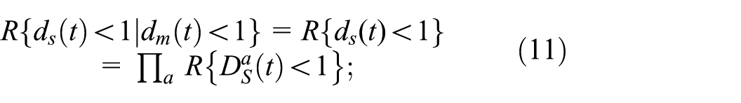
Figure 8 illustrates the evolution of damage distribution for selected components over time. Due to the substantial variation in the probability density f of damage across different operating durations, a transformation $\ln (1 + f)$ was applied to enhance visual clarity. The color gradient in the figure corresponds to values of $\ln (1 + f)$ . As evident from the figure, the damage distribution exhibits a clear trend of increasing dispersion over time.

Figure 8.

Damage distribution of critical components over time: (a) damage distribution of main bearing shell, (b) damage distribution of connecting rod big bearing shell, (c) damage distribution of piston ring and (d) damage distribution of exhaust valve.

Characteristic quantities of the damage distribution functions—for the cylinder liner, piston ring, and exhaust valve—were characterized over time, as illustrated in Figure 9.

Figure 9.

Characteristics quantities of the component damage distribution function over time: (a) Mu and sigma of cylinder liner damage in the logarithmic scale, (b) mean and SD of cylinder liner damage in the original scale, (c) mean and SD of piston ring damage in the original scale and (d) mean and SD of exhaust valve damage in the original scale.

The damage distribution of the cylinder liner follows a log-normal distribution. The parameters mu and sigma represent the mean and standard deviation (SD) in the logarithmic scale, not those of the original damage values, as shown in Figure 9(a). After conversion, the mean and SD of cylinder liner damage in the original scale are presented in Figure 9(b). In contrast, the damage distribution of the piston ring and exhaust valve follows a normal distribution, as illustrated in Figure 9(c) and (d), where the parameters mean and SD denote the actual damage data.

As the figures show, the mean and SD of the damage for the cylinder liner, piston ring, and exhaust valve all increase over time. The rise in the mean damage level reflects the continuous influence of systematic factors promoting damage accumulation, which aligns with the characteristics of cumulative damage. The expansion in the SD of the damage values—that is, the increasing absolute range of fluctuation—suggests that, in addition to systematic factors, the influence of random factors is also intensifying. This leads to growing disparities in damage values among different samples.

Consistent with the bathtub curve model, the wear process leading to failure can be divided into two phases: a period of slow growth and a period of accelerated development. The slow growth phase corresponds to normal wear. Under regular operating conditions, even with the presence of a lubricating oil film, microscopic contact between component surfaces cannot be entirely prevented, resulting in mild and progressive wear. Wear particles are continuously removed by the circulating engine oil, and the rate of damage accumulation remains very low. As wear advances, increased clearances in friction pairs impair the quality and stability of the oil film. Concurrently, aging of the lubricant and accumulation of contaminants further exacerbate wear, leading to an acceleration in the damage accumulation rate. Larger clearances also allow more pronounced unintended component movements—such as impact and eccentricity—introducing additional sources of random fluctuation. Owing to the large number of damage samples, inherent variabilities—such as microscopic material differences, slight variations in assembly, and minor operational fluctuations—are magnified over time as damage progresses. Even under well-controlled test conditions, these variabilities result in a distribution of service life across individual samples.

The damage mechanism of the full-engine

The full-engine damage samples were derived by computing the damage of each component according to the procedure outlined in Section 2.4. Following a goodness-of-fit chi-square test, it was determined that the full-engine damage conforms to a three-parameter Weibull distribution. Taking the system after 5000 h of operation as an example, the resulting damage distribution is illustrated in Figure 10. Using the same methodology described in Section 2.2, the temporal evolution of the full-engine damage distribution is presented in Figure 11.

Figure 10.

Damage distribution of the full-engine at 5000 h.

Figure 11.

Damage distribution of the full-engine over time.

Reliability analysis of critical components

The reliability R(t) of each critical component was evaluated following the procedure outlined in Step (4) of Section 2.4. The resulting component reliability values after 20,000 h of operation are presented in Figure 12. In this figure, the vertical axis label R represents R(t), is defined as the probability that a component survives (does not fail) beyond a specified operating time t, with the value range of R(t) being 0–1.

Figure 12.

Reliability R of critical components.

By integrating the reliability function given in equation (14), the mean time between failures (MTBF) is obtained. In accordance with the Brazilian standard ABNT NBR 6601-2012 for energy consumption testing of passenger vehicles,⁴⁵ the operating time is converted into equivalent mileage under the FTP75 test cycle. This cycle consists of 1874 s, covers a theoretical distance of 17.77 km, reaches a maximum speed of 91.25 km/h, and maintains an average speed of 34.12 km/h. Using this average speed, the MTBF values of components—including the cylinder liner, piston ring, crankshaft, main bearing shell, cam, and exhaust valve—are converted into mileage-based reliability metrics, as summarized in Table 5.

Table 5.

MTBF of critical components.

Components	MTBF (h)	MTBF (km)
Cylinder liner	10,230	349,000
Piston ring	7092	242,000
Crankshaft	35,800	1,221,000
Main bearing shell	12,390	423,000
Cam	15,010	512,000
Exhaust valve	10,110	345,000

The MTBF calculation results reveal significant reliability differences among various key components, particularly with the crankshaft having a much higher reliability than other parts. This phenomenon holds significant engineering implications: it accurately reflects the actual working load and failure mechanisms of different components in the engine. As a core load-bearing component, the crankshaft has a larger design safety margin, thus its reliability is higher; while parts like piston rings and exhaust valves are directly exposed to extreme thermal-mechanical-chemical coupling environments and are typical wear-and-tear components, so their MTBF is much lower, and their lifespan often determines the overhaul cycle. Based on this, the author has two suggestions:

When designing engines, resources should be tilted towards low-reliability components, and efforts should be made to increase the lifespan of these wear-and-tear parts, such as by changing materials, improving processes, and innovating structures.

When maintaining engines, piston rings and similar parts should be the focus of monitoring. A predictive maintenance system should be established through means such as oil analysis and parameter monitoring, and these components should be managed as critical parts. For high-reliability components like the crankshaft, the maintenance focus should be on ensuring their ideal working environment.

Reliability analysis of the full-engine

Following the procedure outlined in Step (5) of Section 2.4, the full-engine reliability R(t) was derived from the reliability values of individual components. The resulting reliability curve of the mechanism model is presented in Figure 13.

Figure 13.

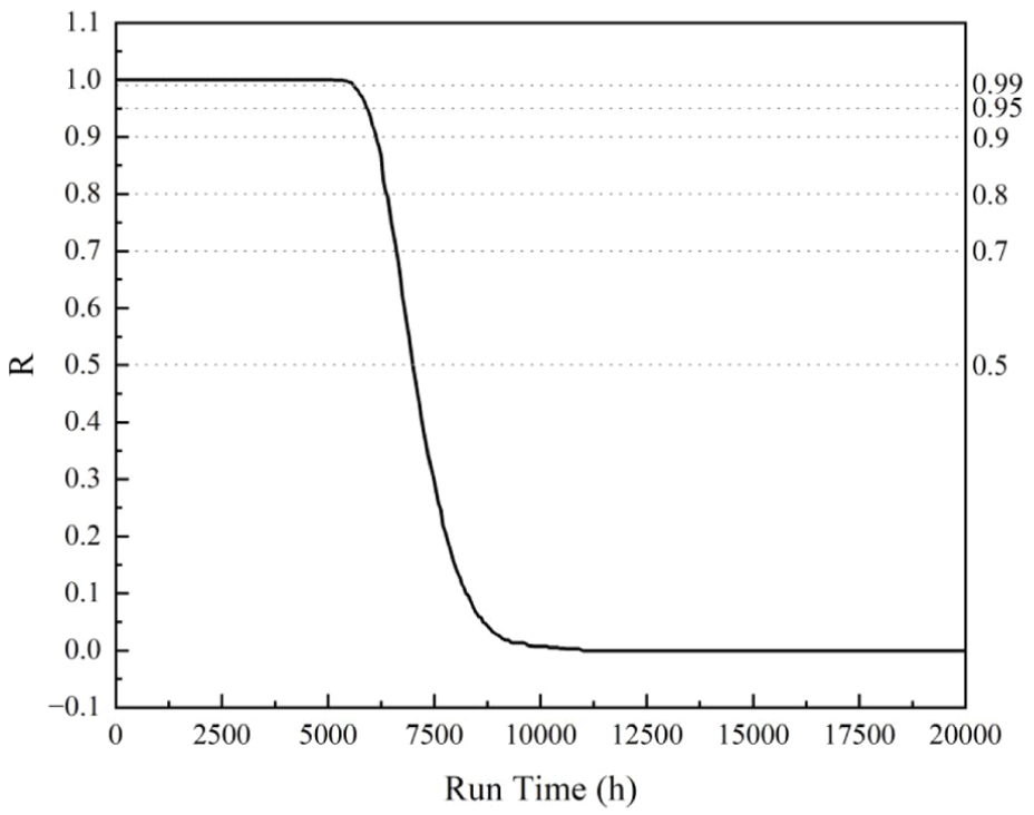
Full-engine reliability R of the mechanism model.

The full-engine MTBF of the mechanism model was computed to be 7091 h, equivalent to ∼242,000 km based on the FTP75 test cycle conversion. Furthermore, the service life corresponding to a specified reliability level R can be determined from the reliability curve, as summarized in Table 6.

Table 6.

Full-engine lifetime under specified reliability requirements.

Reliability	Life (h)	Life (km)
0.99	5549	189,000
0.95	5850	200,000
0.9	6050	206,000
0.8	6263	214,000
0.7	6433	219,000
0.5	6674	228,000

The time at which the reliability decreases to 0.9 is referred to as the B10 life of the product. In general, inspection and warranty services should be performed when the B10 life is reached. For this model, the B10 life is 6050 h, equivalent to ∼206,000 km. To ensure operational usability, it is recommended to maintain reliability at 0.9 or slightly lower (e.g. 0.8). The maximum allowable operating time for this model is 6263 h, or about 214,000 km. The operating time corresponding to a reliability level of 0.5 is termed the B50 life (median life), representing the average life expectancy of the product. Half of the samples in a population are expected to reach this life. For this engine model, the average life is 6674 h, ∼228,000 km.

In addition to the critical components previously discussed, failures in core subsystems—such as the fuel injection system, turbocharger system, cooling system, lubrication system, and electronic control system (ECU and sensors)—also significantly influence full-engine reliability. Based on historical reliability data from manuals of a comparable automobile diesel engine model and studies cited in relevant literature,^46–50 the failure rates for these subsystems were obtained, as summarized in Figure 14.

Figure 14.

Failure rates of engine subsystems.

The reliability R(t) derived from the mechanism model was integrated with the prior failure rate data of the subsystems presented in Figure 14, using equation (10), under the assumption that all components and subsystems are connected in series, the resulting system-level reliability curve for the full-engine is shown in Figure 15.

Figure 15.

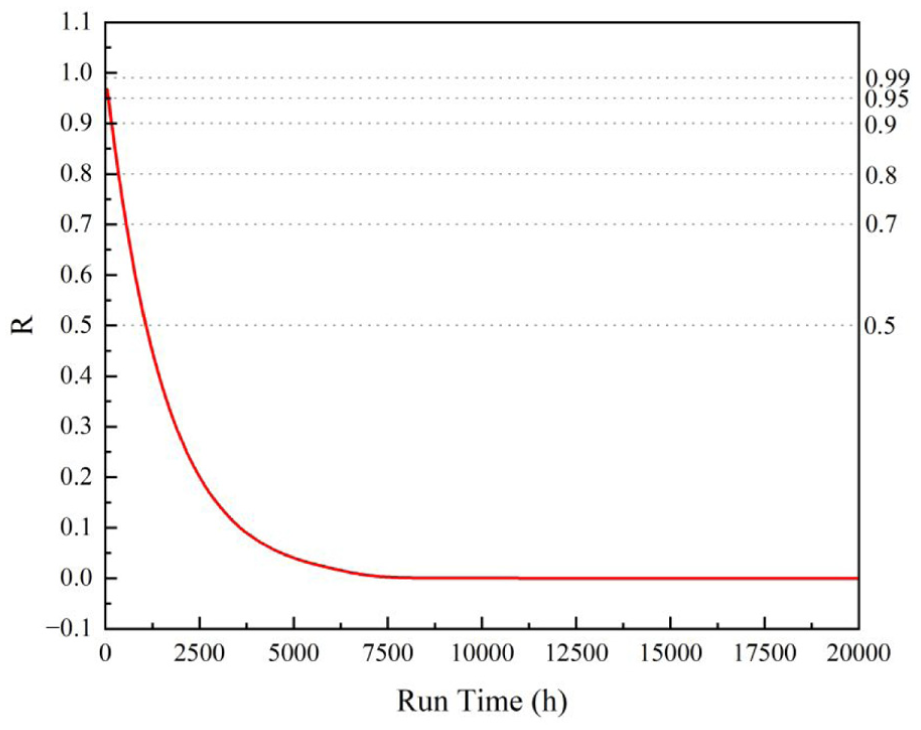
Full-engine reliability R integrating subsystem failure rates.

The MTBF of the integrated full-engine system is 1490 h, equivalent to ∼50,000 km. Compared to the pre-integration model, the full-engine system lifespan shows a significant decrease after integration. To improve engine durability, it is recommended to implement timely inspection and maintenance protocols.

As shown in Figure 14, the failure rates of the cooling system and the lubrication system are the highest, and their impact on the overall reliability of the engine is relatively large. To enhance the reliability of these two subsystems, based on existing research,^51–53 several methods can be adopted:

For the cooling system, high-quality radiators can be used to ensure sufficient heat dissipation capacity and flow; regular inspection and replacement of coolant should be carried out to prevent coolant deterioration and a decline in cooling performance; intelligent temperature control systems can be installed to dynamically adjust the cooling intensity and avoid overcooling or overheating; multi-sensor signal multi-scale fusion fault detection methods can be introduced for predictive maintenance.

For the lubrication system, high-performance lubricating oil can be selected and the lubrication environment optimized; efficient oil filters can be adopted to effectively remove impurities and wear particles from the oil; the oil circuit design can be optimized to ensure that all moving parts receive adequate lubrication; engine vibration signals can be analyzed to identify faults such as bearing wear caused by poor lubrication and intervene at an early stage.

Conclusion

This study investigates the reliability of an automobile diesel engine by introducing a novel framework that combines mechanistic modeling with statistical data analysis. Based on this approach, the following conclusions are derived:

Mechanism model was established for performance computation, crank-connecting rod dynamics, and damage computation. The reliability of an automobile diesel engine was investigated through the integration of mechanistic modeling and statistical data analysis. Additionally, a simplified graphical modeling tool was developed to support pre-processing tasks.

To verify the proposed wear model, a reliability test bench was set up. A certain vehicle diesel engine was subjected to a 300-h wear test at the operating point of 2200 r/min and 600 Nm. The error between the calculated wear weight of the main bearing bush and the measured value was 2.03%, which was relatively small, indicating that the model had a high degree of accuracy.

The damage distributions of critical components—including the cylinder liner, piston ring, crankshaft, connecting rod big-end bearing shell, cam, exhaust valve, and the full-engine—were computed using the developed model. Using 5000 h of operation as an example, the damage distribution of the cylinder liner and crankshaft follows a log-normal distribution, while that of the piston ring, cam, and exhaust valve follows a normal distribution. The damage of the full-engine system conforms to a three-parameter Weibull distribution. The wear behavior of the cylinder liner exhibits characteristics of cumulative damage, with a steadily increasing central tendency and essentially stable relative dispersion. In contrast, both the piston ring and exhaust valve show a continuous rise in mean damage levels under persistent systemic influences. Furthermore, the absolute fluctuation in damage values has widened due to random factors, leading to increasingly significant variations among individual samples. Overall, the distributions of damage across both components and the full-engine system become increasingly dispersed over time, a trend that aligns with objective physical principles.

The reliability curves of the components and the full-engine system align with the bathtub curve trend, exhibiting both a slow growth period and an accelerated development period. The B10 service life of this diesel engine is 6050 h (∼206,000 km), while the B50 life is 6674 h (∼228,000 km). After integrating the subsystem failure rates, the MTBF of the full system is significantly reduced to 1490 h, or roughly 50,000 km.

Footnotes

Handling Editor: Chenhui Liang

ORCID iD

Haiyong Peng

Funding

The authors received no financial support for the research, authorship, and/or publication of this article.

Declaration of conflicting interests

The authors declared no potential conflicts of interest with respect to the research, authorship, and/or publication of this article.

References

Tang

, et al. Data-driven fatigue life prediction of small-deep holes in a nickel-based superalloy after a cold expansion process. Int J Fatigue 2024; 181: 108159.

Wang

Zhang

Reliability analysis of heavy-duty truck diesel engine based on after-sales maintenance data. J Fail Anal Prev 2021; 21: 993–1001.

Xie

Wang

, et al. A data-driven approach for reliability assessment and remaining life prediction of aero-engines based on a time-transformed bivariate Wiener process and Copula dependency structure. Aerosp Sci Technol 2025; 168: 111257.

Yuan

Remaining useful life prediction framework of equipment based on improved golden jackal algorithm assisted-LSTM. AIP Adv 2024; 14(1): 015102.

Warter

Laubichler

Kiesling

, et al. Data-driven prediction of key combustion parameters based on an intelligent diesel fuel injector for large engine applications. SAE Int J Adv Curr Pract Mob 2023; 5(6): 2444–2456.

Wei

Xie

Wang

, et al. Research on service life prediction of diesel engine. J Softw Eng 2016; 10(4): 392–399.

Zhang

Jing

Wang

, et al. Mechanism investigation on fatigue failure in threaded hole of the main bearing in high-strength diesel engine. Eng Fail Anal 2023; 143(A): 106921.

Cui

Zhang

Yang

, et al. Residual Lifetime Prediction of A Vehicle Engine Using Fuzzy Similarity Analysis. 2013 International conference on quality, reliability, risk, maintenance, and safety engineering: QR2MSE 2013, Chengdu, China, 15–18 July 2013, pages 1447–2170, [v.3] (pp. 1827–1830). Institute of Electrical and Electronics Engineers.

Liu

Wang

Liu

WH.

Finite element analysis of thermo-mechanical conditions inside the piston of a diesel engine. Appl Therm Eng 2017; 119: 312–318.

10.

Yin

Meng

, et al. Life-cycle wear evolution model for engine Cu-based bushings. Wear 2025; 580–581: 206272.

11.

Wang

Singh

SSK

, et al. Modelling and fatigue reliability investigation on wear prediction of piston/cylinder pair based on friction fatigue mechanism. Tribol Int 2024; 194: 109485.

12.

Dowell

Akehurst

Burke

RD.

Characterisation and optimisation of a real-time diesel engine model. Proc Inst Mech Eng D J Automob Eng 2017; 231(14): 1913–1934.

13.

Ivana

Çağlar

Maja

, et al. Combined fault tree analysis and Bayesian network for reliability assessment of marine internal combustion engine. J Mar Sci Appl 2025; 25(2): 692.

14.

Zhang

Guo

GY.

Surplus fatigue life prediction of diesel engine piston by the equivalent J-integral approach. Adv Mater Res 2011; 399–401: 2305–2308.

15.

Zhu

Wang

Jia

, et al. Fatigue analysis of marine diesel engine crankshaft. J Phys Conf Ser 2022; 2336(1): 012006.

16.

Wang

Liu

, et al. Numerical study on fretting wear of mating surface between piston crown and skirt in heavy duty diesel engine. J Eng Gas Turbines Power 2019; 141(8): 74.

17.

Cao

Xiao

Sun

, et al. A hybrid data- and model-driven learning framework for remaining useful life prognostics. Engineering Applications of Artificial Intelligence 2024; 135: 108557.

18.

Pulpeiro

Ankobea

Peng

, et al. On the integration of physics-based and data-driven models for the prediction of gas exchange processes on a modern diesel engine. Proc Inst Mech Eng D J Automob Eng 2021; 236(5): 857–871.

19.

Xiao

Wang

ZX.

IndRNN-based data-driven modeling integrated with physical knowledge for engine performance monitoring. J Eng Gas Turbines Power 2024; 147(2): 021012.

20.

Lang

Bloch

Koch

, et al. Application of a combined physical and data-based model for improved numerical simulation of a medium-duty diesel engine. Automot Engine Technol 2019; 5(1–2): 1–20.

21.

Marvin

Anne

System reliability theory models, statistical methods, and applications. 3rd ed. John Wiley & Sons, Inc., 2021.

22.

Chen

Zhang

Deng

, et al. Real-time engine model development based on time complexity analysis. Int J Engine Res 2022; 23(12): 2094–2104.

23.

Feng

Wang

Gao

, et al. A zero-dimensional mixing controlled combustion model for real time performance simulation of marine two-stroke diesel engines. Energies 2019; 12(10): 2000.

24.

Chalet

Yassine

Migaud

New 0D/1D physical approach for modelling the gas dynamics behavior inside the intake system of an engine. J Therm Sci 2018; 27(4): 394–403.

25.

Marinoni

Tamborski

Cerri

, et al. 0D/1D thermo-fluid dynamic modeling tools for the simulation of driving cycles and the optimization of IC engine performances and emissions. Appl Sci 2021; 11(17): 8125.

26.

Zhang

Shen

, et al. Development of a zero-dimensional model for a low-speed two-stroke marine diesel engine with exhaust gas bypass and performance evaluation. Processes 2023; 11(3): 936.

27.

Hernandez-Comas

Maestre-Cambronel

Pardo-Garcia

, et al. Influence of compression rings on the dynamic characteristics and sealing capacity of the combustion chamber in diesel engines. Lubricants 2021; 9(3): 25.

28.

Zhang

, et al. Evolution mechanism of wear characteristics of cylinder liner and piston ring under starved lubrication condition. Tribol Int 2025; 208: 110622.

29.

Archard

JF.

Contact and rubbing of flat surfaces. J Appl Phys 1953; 24(8): 981–988.

30.

Yan

Tong

Zhang

, et al. Research on accelerated thermal fatigue testing and life prediction of Al–Si alloy pistons under start–stop cycles. Int J Fatigue 2025; 191: 108677.

31.

Zhang

Cui

Liang

, et al. Fatigue life prediction analysis of high-intensity marine diesel engine cylinder head based on fast thermal fluid solid coupling method. J Braz Soc Mech Sci Eng 2021; 43(6): 327.

32.

Andrei

Diesel engine engineering. 2nd ed. King Printing Company, Inc., 2011.

33.

Gujar

Bhaskar

SV.

Shaft design under fatigue loading by using modified Goodman method. Int J Eng Res Appl 2013; 3(4).

34.

Usabiaga

Muniz-Calvente

Ramalle

, et al. Improving with probabilistic and scale features the Basquin linear and bi-linear fatigue models. Eng Fail Anal 2020; 116: 104728.

35.

NSWC-10. Handbook of reliability prediction procedures for mechanical equipment. NSWC, 2010.

36.

Ebeling

CE.

An introduction to reliability and maintainability engineering. Waveland Press, Inc., 2009.

37.

Elsayed

Reliability engineering. John Wiley & Sons, Inc., 2009.

38.

Song

Kawai

Monte Carlo and variance reduction methods for structural reliability analysis: a comprehensive review. Probabilist Eng Mech 2023; 73: 103479.

39.

Rubinstein

Kroese

DP.

Simulation and the Monte Carlo method. Wiley, 2016.

40.

Liu

Chen

The fuzzy reliability calculation for cylinder liner wear life of internal combustion engine. Appl Mech Mater 2013; 2746(423–426): 1978–1981.

41.

Miner

MA.

Cumulative damage in fatigue. J Appl Mech 1945; 12(3): 159–164.

42.

Huang

Zhu

, et al. A modified nonlinear fatigue damage accumulation model. Int J Damage Mech 2015; 24(2): 168–181.

43.

Zogu

Schafer

Reliability assessment of composite column according to Monte Carlo simulation and Latin hypercube sampling. E3S Web Conf 2024; 550: 1037.

44.

Pearson

Magnello ME

, Karl. In: Armitage

Colton

(eds Encyclopedia of Biostatistics. John Wiley & Sons, Ltd. 2005, pp.724–731.

45.

ABNT NBR 6601-2012 Light Motor Road Vehicles- Determination of Hydrocarbons, Carbon Monoxide, Nitrogen Oxides, Carbon Dioxide and Particulate Matter in Exhaust Gas. Rio de Janeiro: Associação Brasileira de Normas Técnicas (ABNT), 2012.

46.

Quang

TDP

Phat

Quan

, et al. An image-classifying-based diagnostic method applied to electronic fuel injection system for gasoline engine. J Phys Conf Ser 2025; 2949: 012068.

47.

Niknafs

Zarepour

Faridkhah

Design of an expert system based on fuzzy logic for real-time oil condition monitoring and fault diagnosis in heavy-duty diesel engines. Int J Qual Eng Technol 2023; 9(3): 211–239.

48.

Wang

Stetsyuk

, et al. Exploiting Bayesian networks for fault isolation: a diagnostic case study of diesel fuel injection system. ISA Trans 2019; 86: 276–286.

49.

Saiful

Husaini Nurdin

Failure analysis on the fracture shaft of a centrifugal pump used for diesel engine cooling system. Key Eng Mater 2021; 6229: 107–114.

50.

Inshakov

Kuvshinov

Kornaukhov

OF.

Integrated approach to the diagnostics of tractor diesel turbocharger systems. Tract Agric Mach 2012; 79(10): 15–16.

51.

Liang

Mao

Liu

, et al. Multi-sensor signals multi-scale fusion method for fault detection of high-speed and high-power diesel engine under variable operating conditions. Eng Appl Artif Intell 2023; 126: 106912.

52.

Coelho

RNC

Macedo

Quaresma

JNN

. Monitoring the operational condition of a diesel engine by evaluating the parameters of its thermodynamic operation cycle. J Braz Soc Mech Sci Eng 2023; 45(9): 447.

53.

Zhang

, et al. Priori-distribution-guided adaptive sparse attention for cross-domain feature mining in diesel engine fault diagnosis. Eng Appl Artif Intell 2024; 132: 107975.

Reliability prediction of automotive engines integrating mechanism model

Abstract

Keywords

Introduction

Methods

Performance computing and dynamic computing model of the engine

Mechanism model of critical components

Statistical model of critical components

Integrated mechanistic–statistical modeling

Sample generation using the Monte Carlo simulation and Latin hypercube sampling

Reliability analysis of a certain automotive diesel engine

Performance computation and law of degradation

The damage mechanism of critical components

The damage mechanism of the full-engine

Reliability analysis of critical components

Reliability analysis of the full-engine

Conclusion

Footnotes

ORCID iD

Funding

Declaration of conflicting interests

References