An improved WGS-CNN mechanical fault diagnosis model for complex multi-working conditions

Abstract

To address multiple faults and fault severity detection under complex operating conditions such as strong noise, strong time variation and cross-working conditions, traditional CNNs, and wavelet-CNN hybrids often suffer from low accuracy and poor generalization, as they either adopt offline wavelet denoising or use fixed wavelet kernels, leading to lost adaptability. WGS-CNN is proposed with three synergistic mechanism-level innovations, forming a closed-loop design rather than a simple component combination. Multi-scale wavelet initialization with retained backpropagation anchors time-frequency prior knowledge, while enabling adaptive learning, laying a targeted foundation for feature extraction. Building on this prior injection, adaptive Gaussian windows with learnable scale factors dynamically constrain convolutional kernels to align with varying fault features, breaking static filtering limitations. Finally, square function activation fused with Gaussian denoising inherits the constrained features to integrate power spectrum enhancement, strengthening weak fault signals. Experiments show WGS-CNN achieves over 87% F1 across complex scenarios, outperforming traditional CNNs and existing wavelet-CNN hybrids in accuracy and lightweight performance, providing an effective end-to-end solution with fundamental innovations in wavelet-deep learning fusion.

Introduction

In modern industry, the running state of rotating machinery and equipment is very important, and its fault diagnosis has always been the core topic of research, especially under complex conditions such as strong noise, strong time-varying and multi-working condition transfer learning, which is the difficulty and hot spot of current research. ¹ He ² uses the improved time-shift multi-scale fractional fuzzy dispersion entropy and refined time-shift multiscale fractional order fuzzy dispersion entropy and hybrid kernel ridge regression (RTSFFDE-HKRR) to improve the accuracy of fault detection. Zhang et al. ³ proposed a strongly coupled Duffing-van der pol Sr system (SCD-VSR) to enhance the anti-noise performance of the model. Feng et al. ⁴ uses digital twin system to reflect the running state of gearbox. The above research mainly depends on the model and experience, which not only requires high knowledge reserve of the diagnosticians, but also is time-consuming and difficult to find potential faults in time.

With the development of sensing technology and data acquisition technology, the fault diagnosis method based on vibration signal feature transformation and decomposition has gradually become a research hotspot. ⁵ The vibration signal contains abundant information about the running state of the equipment, and the fault of the equipment can be effectively identified by time-frequency analysis, such as Fourier transform (FT), ⁶ wavelet transform (WT), ⁷ and variational mode decomposition (VMD). ⁸ These methods are based on the state information released by the mechanical equipment during operation. ⁹ They have a solid theoretical foundation and do not need to establish a mathematical model for the system. However, their diagnostic process (feature learning, selection and pattern recognition) requires human participation and does not have the ability of incremental and adaptive learning.

In recent years, intelligent fault diagnosis methods based on machine learning have become a hot topic. ¹⁰ By learning knowledge from historical data, the dependence on expert experience is reduced to a certain extent, and the intelligent diagnosis of faults is realized. ¹¹ Typical methods include Support Vector Machine (SVM), ¹² K-nearest neighbor (KNN), ¹³ random forest, ¹⁴ Bayesian, ¹⁵ Linear Discriminant Analysis (LDA), ¹⁶ and so on. These models are shallow models, which are only suitable for small and medium-sized data sets, and lack end-to-end and adaptive learning ability.

With the development of deep learning, many deep models have emerged for intelligent fault diagnosis of rotating machinery. ¹⁷ For example, autoencoder (AE), ¹⁸ restricted Boltzmann machine (RBM), ¹⁹ Convolutional Neural Networks (CNN), ²⁰ Graph Neural Networks, (GNN), ²¹ Recurrent Neural Network ²² (RNN), Long Short-term Memory (LSTM) network ²³ or Gated Recurrent Unit ²⁴ (GRU), Transformer, ²⁵ etc. The vibration signal is a one-dimensional time series data, with fault characteristics often manifesting as local features (such as short-term impacts and periodic fluctuations). While all the aforementioned models have been applied to fault diagnosis, not all of them are well-suited for extracting vibration signal features.

AE and RBM rely on the full connection layer to learn global features, and are insensitive to local fault features. GNN needs to construct graph structure, which is complicated in preprocessing and has poor adaptability to continuous time series. RNN, LSTM, GRU, and Transformer ²⁶ are better at capturing global time dependence and less sensitive to local features. CNN, especially 1-D CNN, has strong local abstraction ability and adaptive learning ability of one-dimensional vibration signals, and has excellent performance in extracting local features and classification. This paper mainly studies the fault diagnosis method based on 1-D CNN, which is described by CNN in the following.

The convolutional kernel of traditional CNN is usually initialized randomly,^27–29 resulting in poor time-frequency locality and multi-resolution capabilities, making it unable to effectively learn non-stationary, time-varying fault features. In contrast, traditional time-frequency analysis methods, particularly wavelet transform (WT), are characterized by their multi-resolution and localization capabilities, making them more effective in handling non-stationary, time-varying signals.

In recent years, many fault diagnosis methods combining wavelet kernels and CNN have emerged, which have significantly improved the accuracy and efficiency of fault identification. Ganguly et al. ³⁰ proposed Wavelet CNN (W-CNN), which uses Gaussian, Mexican and other wavelets to initialize the CNN convolutional kernel, thereby improving the diagnostic accuracy of the model. Li et al. ³¹ proposed the Wavelet Kernel Network (WKN), which uses wavelet kernel to replace the traditional randomly initialized convolutional kernel, and adaptively learns the scale parameters and translation parameters of the wavelet kernel. Yuan et al. ³² further strengthened the mathematical constraints of WKN, so as to improve its characteristics such as vanishing moment and tight support.

Although the above research has improved the diagnostic performance of CNN to some extent and provided corresponding physical explanations, there are still some shortcomings. Existing wavelet-CNN hybrid methods suffer from two critical limitations that hinder their performance under complex working conditions:

• (1) WD-CNN ³³ adopts wavelet denoising as a preprocessing step and random initialization for convolutional kernels, failing to integrate wavelet’s time-frequency prior knowledge into the network’s end-to-end learning;

• (2) Wavelet Scattering CNN ³⁴ replaces trainable convolutional kernels with fixed wavelet kernels, lacking the adaptive ability of backpropagation; WaveNet ³⁵ did not adopt this alternative design, but the wavelet transform is only an independent cross modal fusion module and does not cooperate with convolutional layer adaptive learning, losing flexibility when facing time-varying fault features;

• (3) Gaussian filtering in traditional methods is applied as an offline signal preprocessing step, rather than a dynamic constraint module coupled with convolutional kernels, leading to poor adaptability to cross-working condition feature shifts.

Aiming at these shortcomings, a dynamic collaborative diagnosis model (Wavelet Transform, Gaussian Window, Square, and CNN, WGS-CNN) based on ELCNN ²⁸ is proposed. The model innovatively integrates wavelet initialization, adaptive Gaussian window and square activation function into an integrated mechanism (rather than a simple component combination). The model realizes the synergy of prior knowledge injection and adaptive feature learning. Specifically, the research work of this paper includes the following aspects.

Firstly, the convolutional kernel is initialized by wavelet kernel, so that the model can get a relatively good starting point at the initial stage of training without destroying its adaptive learning characteristics. Secondly, the Gaussian adaptive window function is loaded on the convolutional kernel to add dynamic constraint to it, so that the convolutional kernel can keep localization and multi-resolution in adaptive learning. Finally, the square function is used to replace the traditional activation function, highlighting the contribution of main feature frequencies to classification.

In order to verify the proposed WGS-CNN effect, this paper selects two public bearing data sets for experiments. The experimental results show that WGS-CNN has remarkable diagnostic performance and generalization ability under the conditions of strong noise, strong time-varying and multi-condition transfer learning.

The structure of this paper is as follows: In Section 2, WGS-CNN is introduced to improve the model performance under complex working conditions. Section 3 describes the source of experimental samples and the model parameters. Section 4 evaluates the effectiveness and superiority of WGS-CNN by using public data sets. In Section 5, the advanced nature of the proposed model is evaluated by comparing the performance of various improved CNNs. Finally, Section 6 summarizes the main contributions and innovations of this article.

WGS-CNN improved for complex working conditions

Aiming at the complex working conditions such as strong noise, strong time-varying and multi-conditional transfer learning, the WGS-CNN based on wavelet transform and power spectrum to improve convolutional layer is proposed. As shown in Figure 1, WGS-CNN has optimized the traditional convolutional layer, which mainly includes the following three improvements.

Figure 1.

WGS-CNN network structure and improved convolution layer.

Firstly, the convolutional kernel is initialized by a wavelet kernel, which makes the network have the feature extraction ability with a high starting point.

Secondly, a Gaussian window is introduced into the convolutional kernel to enhance its ability of local feature extraction.

Finally, the features learned by the convolutional kernel are squared to further enhance the main frequency features that contribute to classification.

Convolutional kernel initialized by multiscale wavelet

CNN has powerful feature extraction ability, and its core component is convolutional layer, and the calculation formula is as follows.

$$y(t)=\sum _{i=0}^{L-1}x(t+i)\omega (i)=\mathbf{X}*\mathbf{W}$$

(1)

Where $y(t)$ is that convolutional output at the position $t$ , $x(t)$ is the value of the input signal at the position $t$ , $\omega (i)$ is the value of the convolutional kernel at the position $i$ , and $L$ is the convolutional kernel length. The above convolutional kernels are randomly initialized and lack prior knowledge. For vibration signals with significant local features, the feature learning process of randomly initialized convolutional kernels ( $\omega$ ) is blind, resulting in low learning efficiency.

In contrast, any wavelet basis function has two universal theoretical properties:

• (1) Time-frequency localization

Unlike the Fourier transform that only provides global frequency information, all wavelets can focus on both time and frequency domains. For non-stationary fault signals such as periodic bearing impact pulses, this lets initialized convolution kernels “lock” the time-domain position of fault impacts and the frequency-domain distribution of fault characteristic frequencies, avoiding the blindness of random initialization in feature learning.

• (2) Multi-scale analysis capability

Adjusting the wavelet scale parameter $a$ enables flexible coverage of different frequency bands, which aligns with the hierarchical characteristics of cross-condition fault signals: small scales (e.g. $a$  = 1, 2) have high time resolution, fitting high-frequency weak fault features (e.g. initial crack impacts) under low loads; large scales (e.g. $a$  = 4, 8) have high frequency resolution, suiting low-frequency stable fault features (e.g. spalling vibrations) under high loads. This multi-scale adaptability ensures that, regardless of wavelet type, initialized convolution kernels can match the frequency distribution of fault signals across working conditions, laying a theoretical foundation for cross-condition feature extraction.

Leveraging these universal properties, the WGS-CNN initializes its convolutional kernels with wavelet functions without restricting to a specific type, integrating wavelets’ time-frequency analysis capability into the network’s bottom-level feature extraction. This provides time-frequency prior information support for feature learning in cross-condition transfer fault diagnosis tasks. As the sliding process of convolutional kernels already achieves full spatial scanning of signals which overlaps with the function of the translation factor while the scale factor regulates the width of wavelet functions facilitating the capture of multi-frequency features in signals only the scale parameter is retained for wavelet initialization. Formally the wavelet basis function ${\psi }_a\left(t\right)$ is defined as its expression after scaling with the scale parameter is:

$${\psi }_a\left(t\right)=\frac{1}{\sqrt{\left|a\right|}}\psi \left(\frac{t}{a}\right)$$

(2)

The discrete wavelet ${\psi }_a\left(n\right)$ is used to initialize the convolutional kernel $\omega (n)$ , with its expression as follows:

$$\omega (n)={\psi }_a\left(n\right)=\frac{1}{\sqrt{\left|a\right|}}\psi \left(\frac{n}{a}\right),n=0,1,···N$$

(3)

Where $N$ denotes the length of the convolutional kernel, and $n$ represents the time-domain position in convolutional kernel.

To cover the main frequency range of the signal, the scale factor adopts an equal-interval initialization strategy, generating n scale factors within the range [ $a_{\min }$ , $a_{\max }$ ].

$$a_c=a_{\min }+\frac{(a_{\max }-a_{\min })·(c-1)}{C-1},c=1,2,···,C$$

(4)

Where $a_{\min }$ and $a_{\max }$ are the minimum and maximum scales preset according to the fault characteristic frequency range, and $C$ denotes the number of scales. Notably, both wavelet functions and CNN kernels are rooted in the “sliding inner product” operation. This structural congruence enables wavelets’ time-frequency localization capability to be directly embedded in the underlying convolutional kernels, allowing the network to anchor fault-related features such as the transience of fault impacts and the concentration of frequency energy from the very start of training. This effectively circumvents the inefficiency issue inherent in traditional random initialization.

To verify the effectiveness of the wavelet initialization strategy and confirm the learning reliability of convolutional kernels as well as the quality of output features, experimental verification proceeds from two core dimensions convolutional kernel stability and feature learning quality. Visual comparison and quantitative analysis demonstrate the advantages of wavelet initialization over traditional random initialization.

• (1) Stability of Convolutional Kernels

The training stability of convolutional kernels directly affects feature learning consistency. In cross-condition diagnosis, common features such as inherent fault frequency patterns serve as the cornerstone of generalization. Excessive morphological fluctuation of convolutional kernels during training not only biases the network’s learning of these common features but also erodes the unified benchmark for feature extraction across conditions, ultimately degrading cross-condition diagnostic performance.

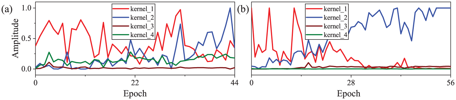
To verify the stability difference between wavelet and random initialization, compare the training changes of convolution kernels under two strategies, Figure 2 (random initialization) and Figure 3 (wavelet initialization).

• (1) Random initialization

Figure 2.

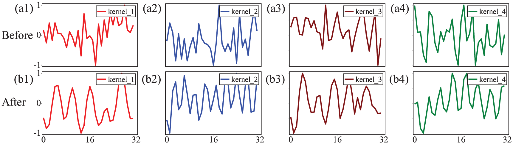
Comparison of time-domain waveforms of convolutional kernels before and after training under random initialization, where (a1–a4) represent convolutional kernels before training; (b1–b4) represent those after training, with the vertical dimension corresponding to four different convolutional kernels in sequence.

Figure 3.

Comparison of time-domain waveforms of convolutional kernels before and after training under wavelet initialization, where (a1–a4) denote convolutional kernels prior to training, (b1–b4) denote those post-training, with the vertical dimension corresponding to four different convolutional kernels in sequence.

Before training, convolutional kernels show a fully disordered, chaotic distribution (Figure 2(a1–a4)), with no tendency to match fault signal features. The network thus lacks a clear learning direction initially and tends to explore invalid feature spaces. After training, while they gradually develop regular fault feature-related morphologies (Figure 2(b1–b4)), revealing only “progressive learning” ability. Their morphology differs sharply from the pre-training state, leading to poor stability.

• (2) Wavelet initialization

Before training, convolutional kernels display the typical morphology of wavelet functions (Figure 3(a1–a4)): a prior structure that naturally aligns with the transient impact features of fault signals. After training, only minor adjustments are made for specific conditions, while their basic morphology remains consistent with the original wavelet function (Figure 3(b1–b4)). This preserves both targeting of fault features and prior stability, fundamentally eliminating meaningless morphological fluctuations of convolutional kernels during training.

To more rigorously quantify the discrepancy in training stability between the two initialization strategies, Table 1, which is specifically titled comparison of correlations of convolutional kernels before and after training under different initialization methods, clearly shows: for the set of randomly initialized convolutional kernels, the average absolute correlation coefficient between their morphological states before and after the full training process is merely 0.19, a value that directly and clearly reflects extremely low correlation between initial and final kernel structures. In sharp contrast, the average absolute correlation coefficient of wavelet-initialized convolutional kernels attains 0.92, demonstrating a significantly higher degree of consistency and correlation between their pre-training and post-training morphological characteristics. This notable gap strongly suggests wavelet-initialized kernels exhibit far greater stability and continuous morphological evolution during the entire feature learning process, compared to their randomly initialized counterparts distinctly lacking such consistency.

• (2) Quality of learned fault features

Table 1.

Comparison of correlation between convolutional kernels before and after training under different initialization methods.

		Convolutional kernel correlation coefficient before and after training
No.	Initialization method	Kernel_1	Kernel_2	Kernel_3	Kernel_4	Average absolute value
1	Random	0.18	−0.37	−0.12	0.11	0.19
2	Wavelet	0.93	0.92	0.99	0.85	0.92

The differences in convolutional kernel initialization methods must ultimately be reflected through the quality of the learned features: high-quality features should be characterized by low noise and high concentration of fault information, which is a core prerequisite for subsequent fault diagnosis. This difference can be verified from two aspects: the feature map spectra in Figure 4, and the correlation data between feature maps and the original signal in Table 2.

• (1) Feature map spectra

Figure 4.

Comparison of frequency spectra of convolutional layer channel feature maps under different initialization methods, where (a1–a4) denote feature maps with random initialization, (b1–b4) denote those with wavelet initialization; the vertical dimension corresponds to four distinct channel feature maps.

Table 2.

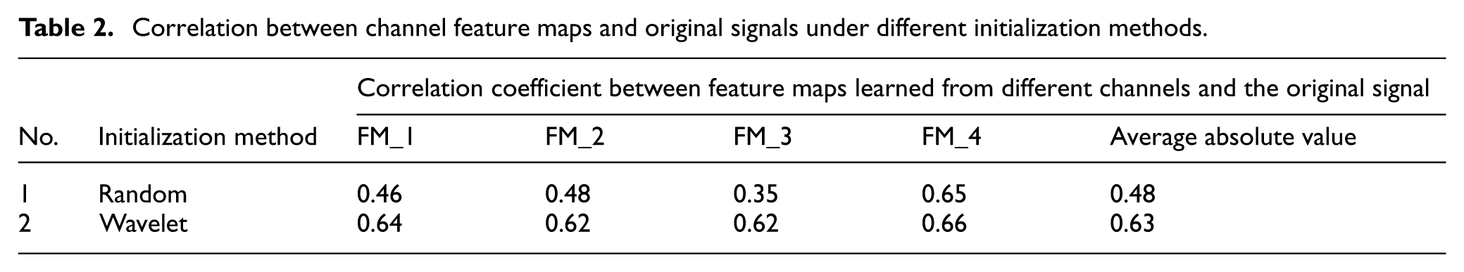
Correlation between channel feature maps and original signals under different initialization methods.

		Correlation coefficient between feature maps learned from different channels and the original signal
No.	Initialization method	FM_1	FM_2	FM_3	FM_4	Average absolute value
1	Random	0.46	0.48	0.35	0.65	0.48
2	Wavelet	0.64	0.62	0.62	0.66	0.63

As can be seen from Figure 4, the feature maps generated by random initialization (Figure 4(a1–a4)) are significantly disturbed by high-frequency noise, with vague feature outlines. In contrast, the feature maps generated by wavelet initialization (Figure 4(b1–b4)) can effectively suppress high-frequency noise and exhibit a more prominent enhancement effect on low-frequency fault features such as the low-frequency components generated by fault impacts, with clearly distinguishable feature outlines.

• (2) Correlation between feature map and original signal

The correlation between the feature maps (FM) obtained via different initialization methods and the original signal (as shown in Table 2) further verifies the above conclusion through quantitative data: the higher the correlation between a feature map and the original signal, the more fully the model retains the original fault information. The average correlation between the features extracted through wavelet initialization and the original signal reaches 0.63, which is significantly higher than the 0.48 of random initialization. This proves that wavelet initialization can effectively enhance the correlation between features and fault information, and that the learned fault features are of better quality.

In summary, unlike existing wavelet-CNNs that rely on fixed wavelet bases and disable backpropagation, the strategy initializes CNN kernels with wavelets while preserving full backpropagation, and its core strength lies in generality as it is compatible with any wavelet that possesses time-frequency localization and multi-scale analysis capabilities, guiding the network to focus on fault features and adapt to complex operating conditions while avoiding the disconnect between offline wavelet denoising and end-to-end learning inherent in WD-CNN. WD-CNN only applies wavelet transform as a preprocessing step without wavelet-based kernel initialization, thus severing the link between wavelet time-frequency analysis and in-network feature learning. Through the synergy of time-frequency prior injection and multi-scale feature extraction, our strategy mitigates the slow convergence of randomly initialized CNN kernels, boosts feature learning efficiency, and provides a time-frequency prior anchor for cross-condition feature alignment in the subsequent learnable window function constraint mechanism, with all these advantages supported by stable learning processes and enhanced feature map quality.

Adaptive-learning Gaussian window function

Wavelet-initialized convolutional kernels introduce prior knowledge to boost a network’s initial feature extraction, yet they limit the network’s flexibility and adaptability to complex conditions. Additionally, adaptive updates of convolutional kernels during training may alter wavelets’ localization traits, weakening their inherent advantages. To resolve this issue, we propose an Adaptive-Learning Gaussian Window, inspired by Morlet wavelets (complex sine wave + Gaussian function), to dynamically constrain convolutional kernels. Below, we elaborate on their integration mechanism and effectiveness across three core sections.

• (1) Theoretical basis

The Morlet wavelet’s dual-localization structure (complex exponential carrier + Gaussian window modulation) offers core theoretical inspiration for combining Gaussian windows with convolutional kernels, as both demand local focusing to accurately extract features from non-stationary fault signals. The specific adaptability is reflected in three aspects.

• (1) Consistency with the “local receptive field” mechanism of convolutional kernels

CNN convolutional kernels extract signal features such as bearing fault transient impact pulses via sliding local receptive fields. Gaussian windows have compact time-domain support with amplitude decaying exponentially with distance from the center, enabling weight modulation for convolutional kernels, thereby enhancing response to central-region fault features while suppressing peripheral noise. This perfectly aligns with kernels’ demand for local feature focusing.

• (2) Adaptability to noise suppression requirements

Rotating machinery vibration signals typically contain high-frequency noise. Gaussian windows exhibit a Gaussian-distributed frequency response with narrow bandwidth and low side lobes, preserving fault-related frequency components while filtering out noise. This avoids “noise overfitting” of convolutional kernels during training and addresses the flaw of randomly initialized kernels prone to learning irrelevant noise.

• (3) Adaptability to dynamic changes in cross-condition signals

Cross-condition fault signals such as the same bearing fault under different rotational speeds exhibit the characteristic that essential fault features such as periodic impacts are stable but the feature frequency shifts proportionally with rotational speed and the time-domain amplitude fluctuates for instance the fault characteristic frequency corresponds to 102.5 Hz at 1730 r/min and slightly shifts at 1797 r/min. The Gaussian window can dynamically adjust the intensity of localization via the variance parameter $\sigma$ : a smaller $\sigma$ improves time resolution, adapting to high-frequency, short-interval impacts under high rotational speeds, while a larger $\sigma$ enhances frequency stability, adapting to low-frequency, long-interval periodic features under low rotational speeds. This adjustability lays a theoretical foundation for the subsequent design of the learnable window function.

• (2) Mathematical Derivation

Taking vibration signals as the research object, the derivation is completed in three steps (window function definition → kernel modulation → convolution calculation) to clarify the mathematical logic of their combination.

• Step 1: Define the Gaussian window function

The expression of the Gaussian window function is:

$$\mathrm{g}(n;\sigma )=\frac{1}{\sigma \sqrt{2\pi }}\exp (-\frac{n^2}{2{\sigma }^2}),n=0,1,···N$$

(5)

Where $n$ denotes the time-domain position of the window function (corresponding to the spatial position of the convolutional kernel), and $\sigma$ is the variance (controlling the window width: a smaller $\sigma$  → narrower window → stronger time-domain localization; a larger $\sigma$  → wider window → stronger frequency stability).

• Step 2: Modulation of the convolutional kernel by the Gaussian window

The Gaussian window is used to weight the parameters ${\psi }_a\left(n\right)$ of the wavelet-initialized convolutional kernel with $n$ denoting the spatial position of the kernel, resulting in the modulated kernel ${\omega }_{\mathrm{G}}(n;\sigma )$ .

$$\begin{array}{c}\multicolumn{1}{c}{{\omega }_{\mathrm{G}}(n;\sigma )={\psi }_a\left(n\right)·\mathrm{g}(n;\sigma )=\frac{1}{\sigma \sqrt{2\pi \left|a\right|}}·\psi \left(\frac{n}{a}\right)·}\\ \multicolumn{1}{c}{\exp (-\frac{n^2}{2{\sigma }^2}),n=0,1,···N}\end{array}$$

(6)

This equation shows that the response of the convolutional kernel is constrained to the central region, and interference from edge noise is suppressed by exponential decay.

• Step 3: Convolution calculation with the modulated kernel

For the input vibration signal $x_t$ (where $t$ is the signal position), the convolution output $y_{\mathrm{t}}$ is:

$$\begin{array}{c}\multicolumn{1}{c}{y(t)=\sum _{i=0}^{k-1}{\omega }_{\mathrm{G}}(n;\sigma )·x(t+i)=\sum _{i=0}^{k-1}\frac{1}{\sigma \sqrt{2\pi \left|a\right|}}·\psi \left(\frac{n}{a}\right)}\\ \multicolumn{1}{c}{·\exp (-\frac{n^2}{2{\sigma }^2})·x(t+i)}\end{array}$$

(7)

Where $L$ is the length of the convolutional kernel. Equation (7) is essentially a “weighted sliding inner product.” The Gaussian window dynamically adjusts the time-frequency response range of the kernel via $\sigma$ , providing mathematical support for adapting to feature frequency shifts in cross-condition scenarios.

• (3) Experimental Validation

To further confirm the rationality of combining Gaussian windows with convolutional kernels, we conducted experiments on a bearing stable rotational speed switching scenario (1730 → 1797 r/min). Three Gaussian window constraint approaches: no Gaussian window, fixed-scale Gaussian window, and learnable-scale Gaussian window were compared. The core value of the learnable window function was verified by analyzing the dynamic evolution of convolutional kernels and the modulation law of feature maps.

• (1) Dynamic Evolution of Convolutional Kernels in Cross-Condition Scenarios

Figure 5 shows the changes in the waveforms of convolutional kernels before and after transfer under different window constraints. “Before transfer” refers to the same working condition (1730 → 1730 rpm), while “Transfer” refers to the cross-working condition (1730 → 1797 rpm). As shown in the Figure 5, the “No Window Transfer” and “fixed-scale Gaussian Transfer” show almost no difference in the waveforms of convolutional kernels before and after transfer (Figure 5(a1–a4) and (b1–b4)), which means they struggle to respond to the feature distribution shift caused by changes in working conditions. In contrast, the “Learnable Gaussian Transfer” leads to significant adjustments to the convolutional kernel waveforms before and after transfer (Figure 5(d1–d4)), and realizes the adaptive reconstruction of the features of the new working condition (1797 rpm) through the dynamic modulation of the window function.

Figure 5.

Comparison of the time-domain waveforms of convolutional kernels before and after transfer under different window constraints, (a1–a4) before transfer, (b1–b4) no window transfer, (c1–c4) fixed Gaussian transfer and (d1–d4) learnable Gaussian transfer.

To quantify this difference, Table 3 calculates the correlation coefficients of convolutional kernels before and after transfer under different window constraints. For the “No Window Transfer” and “Fixed-scale Gaussian Transfer” (which barely adjust with conditions and cannot adapt to new conditions), the average correlation coefficients of their kernels are 0.91 and 0.96 respectively. For the “Learnable Gaussian Transfer,” the average value drops to 0.39, greatly enhancing morphological adjustment. It captures the fault features of 1797 r/min by focusing on the frequency range through dynamic scaling (e.g. shrinking high frequencies and expanding low frequencies).

Table 3.

Correlation coefficients of convolution kernels before and after transfer under different window constraints.

No.	Window constraint method	Correlation coefficients of convolution kernels before and after transfer
		FM_1	FM_2	FM_3	FM_4	Average absolute value
1	No window	0.97	0.89	0.98	0.79	0.91
2	Fixed Gaussian window	0.98	0.99	0.99	0.96	0.98
3	Learnable Gaussian window	0.37	0.26	0.36	0.55	0.39

This result validates the core role of the learnable Gaussian window: by actively adjusting the time-frequency response characteristics of the convolutional kernel, the model can break away from “static feature dependence” during cross-condition transfer, thereby enhancing its adaptability to new working conditions.

• (2) Cross-Condition Modulation of Feature Maps

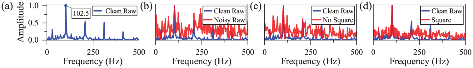
To further verify the optimization effect of the “Learnable Gaussian Transfer” on cross-condition feature extraction, the differences in feature maps learned by the model under different window function constraints were compared. Figure 6 focuses on the target fault frequency of 102.5 Hz, which clearly reflects the impact of different window function modulations on feature extraction.

Figure 6.

Comparison of fault spectra learned by convolution kernels modulated with different window functions: (a) no window transfer, (b) fixed Gaussian transfer and (c) learnable Gaussian transfer.

Firstly, the feature maps of the “No Window” are severely disturbed by high-frequency noise, with the target frequency completely obscured.

Secondly, the “fixed-size Gaussian Transfer” improves SNR to 1.8 and slightly reduces noise, but its fixed scale prevents adaptation to the 102.5 Hz fault frequency. Feature maps show significant shifts in frequency responses of channels (b1) and (b4), with the target fault frequency in purple boxes instead suppressed. This directly reflects that fixed window scales limit feature maps’ ability to focus on the target frequency.

Thirdly, feature maps with the “learnable Gaussian Transfer” show marked quality improvement. For instance, purple boxes in (c1)/(c2) have outstanding noise suppression, with the 102.5 Hz fault frequency showing strong continuity and highly concentrated energy. Even (c3)/(c4), which focus on low-frequency components, still clearly capture the target fault frequency. This advantage comes from its dynamic adjustment: backpropagation-optimized scale parameters ((c1), (c2)) accurately match the 102.5 Hz fault frequency’s bandwidth needs, letting feature maps focus on the target frequency and filter out irrelevant noise.

In conclusion, the combination of Gaussian windows and convolutional kernels forms a complete closed loop from theoretical adaptability and mathematical derivation to experimental validation: the time-frequency localization idea of the Morlet wavelet provides the theoretical origin, mathematical derivation clarifies the computational logic of their combination, and cross-condition experiments further confirm that the learnable window function (with dynamic $\sigma$ adjustment) can effectively enhance the convolutional kernel’s ability to stably capture fault features, providing reliable support for the model’s cross-condition fault diagnosis performance.

Square function of strengthening the main peak frequency

In the field of signal processing, the power spectrum can be used to extract signal features such as peak frequency, which is very useful in pattern recognition and classification. The power spectrum usually represents the power of each frequency component by calculating the amplitude square of the Fourier transform result of the signal. Pang et al. ³⁶ deeply analyzed the output characteristics of CNN convolutional layer, and came to the conclusion that the trained convolutional layer is more inclined to extract frequency domain characteristics. At the same time, Pang pointed out in the research of Pang et al. ²⁸ that the existence of the activation function may lead the model to learn high-frequency features that have little contribution to the classification. Therefore, this paper removes the activation function while increasing the square strategy. Based on the above analysis, the WGS-CNN’s formula for squaring the features extracted from the convolutional layer is as follows.

$$S(F(x))=F(x)F(x)=(x*w)(x*w)$$

(8)

Where $S$ is a square function and $F$ is a WGS-CNN convolutional operation. Different from the Fourier transform, the proposed WGS-CNN convolutional layer has better time-frequency localization characteristics and is more suitable for non-stationary time-varying signal processing.

Based on the improved strategy, WGS-CNN provides a more effective design of convolutional layer by initializing the convolutional kernel with a wavelet kernel, loading an adaptive Gaussian window and squaring its learning characteristics, thus further improving the fault diagnosis accuracy and interpretation ability of the model under complex working conditions. The following part of this paper will verify the effectiveness and superiority of the above strategies through experiments.

Experimental data and model parameters

Data description and preprocessing

In this paper, two published bearing data sets are selected to verify the proposed method. Among them, dataset I is the time-invariant bearing data set provided by Case Western Reserve University (CWRU) in the United States, and dataset II is the time-varying bearing data set provided by University of Ottawa in Canada.

• (1) CWRU Bearing Vibration Data Set

As shown in Table 4, CWRU mainly collects vibration signals of rolling bearings under different working conditions at three kinds of speeds and loads. According to different working conditions, the data set is divided into three subsets (A0–A2). Each subset contains four bearing states, namely, Normal state (N), Inner-race fault (IR), Outer-race fault (OR) and Balls fault (B). The sampling number of each signal is 200, and the sampling frequency is 12 kHz.

Table 4.

CWRU data set description and sample division.

Fault diameter (inches)	Shaft speed (rpm)	Motor load (Hp)	Subset	Status	Sample number	Class labels
0.007	1750	0	A0	N	200	0
				IR	200	1
				OR	200	2
				B	200	3
	1772	1	A1	N	200	0
				IR	200	1
				OR	200	2
				B	200	3
	1797	2	A2	N	200	0
				IR	200	1
				OR	200	2
				B	200	3

In order to evaluate the learning ability of WGS-CNN for complex working condition faults, the experimental data is constructed by first dividing the dataset and then sequentially collecting the data. Specifically, one subset (A0–A2) is selected as the training set, while the remaining subsets are used as the test set. The training set and test set are then sequentially collected.

As shown in Table 5, CWRU includes three bearing failure frequencies: Ball-Pass Frequency of Inner-race (BPFI), Ball-Pass Frequency of Outer-race (BPFO), and Ball Spin Frequency (BSF).

• (2) Ottawa Bearing Vibration Data Set

Table 5.

Description of bearing parameters and bearing fault frequency.

Dataset	Bearing type	Pitch diameter (mm)	Ball diameter (mm)	Number of balls	BPFI	BPFO	BSF
CWRU	6205-2RS JEM SKF	39.04	7.94	9	5.414	3.585	4.724
Ottawa	ER16K	38.52	7.94	9	5.432	3.571	-

As shown in Table 6, the Ottawa bearing dataset primarily acquires and stores vibration signals of rolling bearings operating in distinct health states under four distinct time-varying operating conditions such as varying rotational speeds. Based on the clear variations in these operating conditions, the entire dataset is systematically partitioned into four independent subsets, labeled B0–B3 (i.e. B0, B1, B2, and B3). Each of these four subsets comprehensively encompasses three key bearing health states: N, IR, and OR, ensuring comprehensive coverage of typical bearing failure modes. For each individual vibration signal sample included in the dataset, the number of sampling points is uniformly set to 400, while the sampling frequency is consistently maintained at 200 kHz to capture high-frequency fault characteristics effectively. In line with the data construction protocol of the CWRU dataset, the Ottawa dataset’s experimental data follows a partition-first, then collection approach for consistent construction, ensuring alignment in data organization logic. The bearing failure frequencies in the Ottawa dataset include BPFI and BPFO, as shown in Table 5.

Table 6.

Ottawa data set description and sample division.

Speed varying conditions	Rotation frequency (Hz)	Subset	Status	Sample number	Class labels
Increasing speed	From 14.1 to 23.8	B0	N	400	0
	From 12.5 to 27.8		IR	400	1
	From 14.8 to 27.1		OR	400	2
Decreasing speed	From 28.9 to 13.7	B1	N	400	0
	From 24.3 to 9.9		IR	400	1
	From 24.9 to 9.8		OR	400	2
Increasing then decreasing speed	From 14.7 to 25.3, then to 21.0	B2	N	400	0
	From 15.1 to 24.4, then to 18.7		IR	400	1
	From 14.0 to 21.7, then to 14.5		OR	400	2
Decreasing then increasing speed	From 24.2 to 14.8, then to 20.6	B3	N	400	0
	From 25.3 to 14.8, then to 19.4		IR	400	1
	From 26.0 to 18.9, then to 24.5		OR	400	2

Settings of model parameters

The selection of model parameters directly determines the training efficiency, convergence speed and ultimate performance of the model. This part mainly introduces the structural parameters and training parameters of the model, and the detailed analysis is as follows.

• (1) Model structural parameters

In order to ensure the accuracy and interpretability of the experiment, the structural parameters of WGS-CNN are optimized after 10 repeated experiments. The network structure and its parameters are shown in Table 7.

Table 7.

Network structure parameters of WGS-CNN.

Layer	Kernel size (CWRU/Ottawa)	Kernel number	Output size (CWRU/Ottawa)	Activation function	Bias	Stride	Padding
Conv	32/128	32/8	2048 × 32/32,768 × 8	Square	-	1	Same
Max pooling	2	-	1024 × 32/16,384 × 8	-	-	-	-
GAP	-	-	32 × 1/8 × 1	-	-	-	-
FC	-	-	100 × 1	-	-	-	-
FC	-	-	4 × 1/3 × 1	Softmax	-	-	-

The network structure parameters in Table 7 include sample length, convolutional kernel length, and number. The optimization process is as follows.

• (1) Sample length optimization

The lowest failure frequency of CWRU is the cage failure frequency of 11.93 Hz and the sampling frequency of 12 kHz, from which the length of cage failure signal is calculated to be 1006(12,000 ÷ 11.93 ≈ 1006). In order to ensure the integrity of the data cycle and avoid the marginal effect, we use 2048 as the experimental data length of the CWRU to ensure that the signal sample has more than two cage failure cycles.

The frequency modulation and amplitude modulation components of the bearing signal are usually modulated around the rotation frequency. The minimum rotation frequency of Ottawa is 12.5 Hz, and the sampling frequency is 200 kHz, so the signal length is at least 16,000 (200,000 ÷ 12.5 ≈ 16,000). In order to ensure the integrity of the data cycle and avoid the marginal effect, we use 1024 * 32 = 32,768 as the length of Ottawa’s experimental data to ensure that the signal sample has more than two minimum rotation frequency cycles.

• (2) Optimization of kernel length and number

By optimizing the length and number of convolutional kernels, WGS-CNN achieves more effective feature extraction and model performance on different data sets.

Figure 7 shows the effect of different lengths and different numbers of convolutional kernels on the performance of WGS-CNN on CWRU, (a) is the diagnostic accuracy, and (b) is the model training time. As can be seen from Figure 7(a), the accuracy of model diagnosis increases with the increase of convolutional kernels number. When the number of convolution kernels is 32, the diagnosis accuracy of WGS-CNN using convolution kernels of different lengths can reach 100%. It can be seen from Figure 7(b) that when the number of convolution kernels is 32 and the length is 32, the training time of the model is the shortest (17.28 s) and the variance is relatively small. The optimal length of convolutional kernel of WGS-CNN on CWRU is 32, and the optimal number is 32.

Figure 7.

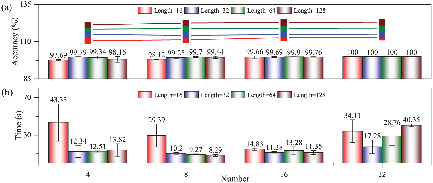
Effect of different lengths and different numbers of convolutional kernels on the performance of WGS-CNN on CWRU: (a) diagnostic accuracy and (b) model training time.

Figure 8 shows the effect of different lengths and different numbers of convolutional kernels on the performance of WGS-CNN on the Ottawa. It can be seen from Figure 8 that when the number of convolution kernels is 8 and the length is 128, the diagnostic accuracy of the model is the highest (98.85%), the training time is relatively short (42.02 s), and the variance is small. It can be seen that the preferred length of the WGS-CNN convolutional kernel on Ottawa is 128 and the preferred number is 8.

• (2) Training parameters

Figure 8.

Effect of different lengths and different numbers of convolutional kernels on the performance of WGS-CNN on Ottawa: (a) diagnostic accuracy and (b) model training time.

As shown in Table 8, WGS-CNN uses Adam optimizer and cross entropy loss function to train. In the iterative training process of the model, the batch is set to 64, and the dynamic learning rate strategy is used to optimize it (initial value is 0.01). In addition, the patient value is set to 10, so that the early stop mechanism can be triggered in time when the model performance is not improved, which can prevent over-fitting and saving training time.

Table 8.

Training parameters of WGS-CNN.

Optimizer	Loss function	Batch-size	Learning rate	Patience
Adam	Cross entropy	64	Dynamic	10

The above dynamic learning rate is adjusted by exponential decay and cosine annealing, and its formula is as follows.

$$r=\frac{r^{\exp }+r^{\cos }}{2}$$

(9)

$$r_i^{\exp }=r_{i-1}^{\exp }{e}^{-0.1}$$

(10)

$$r^{\cos }=0.5r_{\mathrm{initial}}(1+\cos \left(\pi \frac{\mathrm{epoch}}{\mathrm{epochs}}\right))$$

(11)

$r^{\exp }$ is the exponential decay learning rate, $r_{i-1}^{\exp }$ is the last learning rate, $r^{\cos }$ is the cosine annealing learning rate, $r_{\mathrm{initial}}$ is the initial value of the learning rate of 0.01, $\mathrm{epoch}$ is the current training step of the model, and $\mathrm{epochs}$ is the maximum training step of the model of 1000. The above exponential decay and cosine annealing learning rates all adopt the strategy of striding fast in the early stage and jogging in the late stage, so that the model can avoid falling into the local optimal solution.

Verification of effectiveness, superiority and reliability of improved strategy

To verify the effectiveness, superiority, and engineering reliability of the WGS-CNN improved strategy, this section adopts the variable control method, supported by the CWRU (stable working conditions) and Ottawa (strongly time-varying working conditions) bearing datasets. First, ablation experiments and classification visualization are used to verify the independent and synergistic effectiveness of the strategy. Then, horizontal comparison with other mainstream similar strategies is conducted to highlight its performance advantages. Finally, combined with hyperparameter sensitivity analysis, the optimal value range of key parameters is determined, providing a reliable basis for model parameter setting and subsequent performance verification.

Effectiveness analysis of improvement strategies

Different combinations of improvement strategies have different effects, which will be analyzed from two aspects: model diagnosis performance and model classification visualization.

• (1) Diagnostic Performance of Model

In order to simulate strong noise training, Gaussian white noise with signal-to-noise ratio of −10 is added to the experimental samples. In order to simulate multi-conditional transfer training, different subsets of data sets are selected as training set and test set. For example, the CWRU in Table 4 contains three subsets A0, A1 and A2, and different combinations of subsets can be selected to participate in model training and testing. To ensure the reliability of the experiment, two different multi-conditional transfer learning data sets (A0 → A1, A2, A1 → A0, A2) are selected for comparative analysis. In addition, in order to accurately evaluate the performance of the model, accuracy rate (Acc), precision rate (Pre), recall rate (Rec) and F1 score (F1) are introduced to evaluate the classification results. ³⁷

Table 9 shows the performance comparison of different improvement strategies for CWRU-based WGS-CNN. Among them, the blue WGS is the benchmark model without any improvement strategy, and its F1 index in C1 Task is 77.59%, and that in C2 Task is 64.71%. The following is a comparison of other improvement strategies with WGS, and the specific analysis is as follows.

• (1) Effectiveness of using wavelet to initialize the convolutional kernel

Table 9.

Influence of different improvement strategies on the performance of WGS-CNN on CWRU. Red-shaded areas indicate the model with all three improvement strategies, and blue-shaded areas represent the model without any improvement strategy, while unshaded areas correspond to the model with partial improvement strategies. W, G, and S represent different strategies used by the model, where W represents wavelet initialization convolutional kernel, G represents Gaussian window, S represents square function, W represents random initialization convolutional kernel, G represents no window function, and S represents no square function.

No.	Method	Task labels	Data sets (train → test)	Acc (%)	Pre (%)	Rec (%)	F1 (%)	Convergence time (s)
1	WGS	C1	A0 → A1,A2	89.18	77.43	77.83	77.59	64.55
		C2	A1 → A0,A2	81.46	61.86	70.08	64.17	50.41
2	WGS	C1	A0 → A1,A2	94.26	86.84	91.75	89.21	52.94
		C2	A1 → A0,A2	93.76	90.46	84.68	87.25	24.36
3	WGS	C1	A0 → A1,A2	91.17	82.15	82.87	83.88	60.27
		C2	A1 → A0,A2	94.24	90.06	86.48	88.15	52.15
4	WGS	C1	A0 → A1,A2	58.33	8.33	33.33	13.33	11.26
		C2	A1 → A0,A2	58.34	8.32	33.21	13.31	12.65
5	WGS	C1	A0 → A1,A2	95.42	91.21	90.6	90.83	57.98
		C2	A1 → A0,A2	95.09	89.29	92.07	90.64	47.94
6	WGS	C1	A0 → A1,A2	95.73	92.56	90.40	91.40	43.09
		C2	A1 → A0,A2	95.81	93.43	89.80	91.52	42.35
7	WGS	C1	A0 → A1,A2	67.14	12.97	45.01	26.15	14.56
		C2	A1 → A0,A2	65.83	22.20	23.17	17.55	19.00
8	WGS	C1	A0 → A1,A2	95.61	90.89	93.20	92.01	70.81
		C2	A1 → A0,A2	96.21	93.23	91.98	92.53	25.27

The F1 index of WGS with only wavelet initialization convolutional kernel strategy is 89.21% in C1 Task and 87.25% in C2 Task. Its diagnostic performance is higher than that of WGS model (C1 77.59%, C2 64.71%) without improved strategy, and its diagnostic time is shorter. This is because wavelet function has good mathematical definition and good time-frequency localization characteristics, which can give convolutional kernel a better initialization starting point, thus improving fault diagnosis performance faster and better.

• (2) Effectiveness of Gaussian window

The F1 index of WGS with Gaussian window is 83.88% in C1 Task and 88.15% in C2 Task, and its diagnostic performance is higher than that of WGS model (C1 77.59%, C2 64.71%) without improved strategy. Similar to wavelet initialization convolutional kernel strategy, the model uses window function with good time-frequency localization characteristics to dynamically constrain convolutional kernel, which can extract fault features more effectively and improve model diagnosis performance.

• (3) Effectiveness of square function

The F1 index of WGS with square function is 13.33% in C1 Task and 13.31% in C2 Task, and its diagnostic performance is the worst, far lower than that of WGS model (C1 77.59%, C2 64.71%) without improved strategy. However, the F1 index of WGS using Gaussian window and square function is 91.40% in C1 Task and 91.52% in C2 Task, respectively, and its diagnostic performance is higher than that of WGS model. This is because the fault frequency of the signal sample is submerged in the noise under the condition of strong noise, and the square function cannot work. It must be denoised first to extract the fault frequency by square.

It can be seen from Table 9 that the F1 index of WGS marked in red with three improved strategies is 92.01% on C1 Task and 92.53% on C2 Task. The diagnostic performance of WGS on two Task is higher than that of other diagnostic models (WGS, WGS, and WGS) using one improved strategy and two improved strategies (WGS, WGS, and WGS). It is fully demonstrated that the combination of the three improved strategies is effective and can meet the fault diagnosis under strong noise and multi-condition transfer learning.

Table 10 shows the performance comparison of different improvement strategies for Ottawa-based WGS-CNN. The blue model WGS is also the benchmark model without any improvement strategy. Consistent with CWRU, the experiment based on Ottawa can also draw the following conclusions.

Table 10.

Influence of different improvement strategies on the performance of WGS-CNN on Ottawa. Red-shaded areas indicate the model with all three improvement strategies, and blue-shaded areas represent the model without any improvement strategy, while unshaded areas correspond to the model with partial improvement strategies. W, G, and S represent different strategies used by the model, where W represents wavelet initialization convolutional kernel, G represents Gaussian window, S represents square function, W represents random initialization convolutional kernel, G represents no window function, and S represents no square function.

No.	Method	Task labels	Data sets (train → test)	Acc (%)	Pre (%)	Rec (%)	F1 (%)	Convergence time (s)
1	WGS	O1	B0 → B1,B2,B3	55.42	20.11	33.13	24.53	33.83
		O2	B1 → B0,B2,B3	54.86	19.64	32.28	22.35	47.96
2	WGS	O1	B0 → B1,B2,B3	56.93	40.52	35.39	36.11	27.19
		O2	B1 → B0,B2,B3	60.96	44.35	41.32	42.43	43.95
3	WGS	O1	B0 → B1,B2,B3	59.92	44.73	39.88	41.94	72.62
		O2	B1 → B0,B2,B3	62.44	37.02	43.66	40.03	26.92
4	WGS	O1	B0 → B1,B2,B3	55.56	11.11	33.33	16.67	19.11
		O2	B1 → B0,B2,B3	55.56	11.11	33.33	16.67	26.08
5	WGS	O1	B0 → B1,B2,B3	56.93	43.58	39.45	41.23	80.03
		O2	B1 → B0,B2,B3	63.30	39.92	44.95	42.03	58.74
6	WGS	O1	B0 → B1,B2,B3	95.74	94.83	93.61	94.20	164.02
		O2	B1 → B0,B2,B3	93.64	91.92	90.46	91.18	70.39
7	WGS	O1	B0 → B1,B2,B3	55.56	11.11	33.33	16.67	35.69
		O2	B1 → B0,B2,B3	55.86	17.31	33.78	21.05	24.93
8	WGS	O1	B0 → B1,B2,B3	98.08	97.16	97.13	97.14	147.61
		O2	B1 → B0,B2,B3	94.25	92.55	91.38	92.16	129.85

Firstly, using wavelet to initialize the convolutional kernel is also effective under strong time-varying conditions.

Secondly, using Gaussian window to dynamically constrain convolutional kernel is also effective under strong time-varying conditions.

Finally, the combination of square function and Gaussian window is also effective under strong time-varying conditions.

The experimental results and conclusions obtained on Ottawa are consistent with CWRU, which fully demonstrates the universality of our improved strategies.

• (2) Visualization of model classification

In order to further illustrate the effectiveness of the proposed improved strategies, this section uses T-SNE technology to visualize the classification results of different improved strategies on CWRU(A0 → A1,A2), and the specific analysis is as follows.

• (1) Effectiveness of single strategy

The WGS of Figure 9(b), which only uses wavelet to initialize convolution, has better classification effect than the WGS of Figure 9(a), which does not use any strategy (e.g. the green IR fault is better separable). The classification effect of Figure 9(c) WGS with only Gaussian window (such as green inner-loop fault separability) is also better than that of Figure 9(a) WGS without any strategy. The above visual classification results further show the effectiveness of initializing convolutional kernels with wavelet and loading Gaussian windows on convolutional kernels. Figure 9(d) WGS, which only uses the square function, shows that the four types of faults are randomly distributed, and the fault dispersion is the largest, and the classification effect is the worst. Once again, it is proved that it is ineffective to square the noisy samples directly.

• (2) Effectiveness of combined strategy

Figure 9.

T-SNE diagnosis visualization of WGS-CNN on CWRU (A0 → A1, A2) using different improved strategies: (a) WGS, (b) WGS, (c) WGS, (d) WGS, (e) WGS, (f) WGS, (g) WGS and (h) WGS.

Different improvement strategies have different results. Figure 9(e) shows the WGS classification effect of combining wavelet initialization convolutional kernel with Gaussian window, which is obviously better than the model (WGS, WGS) using only a single strategy. Similarly, in Figure 9(f), WGS model successfully separates the orange B faults by using two improved strategies, namely Gaussian window and square function, and its effect is better than that of the single strategy model (WGS, WGS). However, the WGS model in Figure 9(g) does not use Gaussian windows, which leads to the reduction of the effect of the combination strategy, which once again emphasizes the importance of Gaussian windows in smoothing and noise suppression. Finally, Figure 9(h) shows the WGS model using three strategies, which not only successfully separates the faults of B completely, but also makes the other three types of faults more concentrated, showing better separability.

To sum up, the classification results of WGS-CNN on CWRU (A0 → A1, A2) are visualized by T-SNE diagram, which shows that the combination of the three improved strategies is effective.

In order to further prove the effectiveness of the proposed improved strategies, this section uses T-SNE diagram to visualize the classification results of WGS-CNN on Ottawa (B0 → B1, B2, B3), and the specific analysis is as follows.

Consistent with CWRU, the experiment based on Ottawa in Figure 10 can get similar results.

Figure 10.

T-SNE diagnosis visualization of WGS-CNN on Ottawa (B0 → B1, B2, B3) using different improved strategies: (a) WGS, (b) WGS, (c) WGS, (d) WGS, (e) WGS, (f) WGS, (g) WGS and (h) WGS.

Firstly, the classification effect of (b) WGS and (c) WGS of a single strategy is better than that of the benchmark model (a) WGS, and the fault classification effect is worse and the fault distribution is more dispersed without using the Gaussian window to directly square (d) WGS.

Secondly, the blue OR fault of the combined strategy (e) WGS is more concentrated than the benchmark model, while the fault concentration in (f) WGS is higher, showing a thin line state. The combination strategy (g) WGS without Gaussian window has a poor classification effect, while the classification effect of WGS using three strategies is more obvious.

In summary, the visualization results and conclusions drawn from the Ottawa are consistent with those from CWRU, indicating that the proposed improvement strategies are universally applicable.

Horizontal comparative analysis of improvement strategies

In order to verify the advantages of the improved strategies of WGS-CNN, the improved strategies are compared with other similar strategies horizontally. The experimental training samples in this section are consistent with the effectiveness analysis of the improved strategies in the previous section. The data sets of multi-condition transfer learning on CWRU and Ottawa (A0 → A1, A2, B0 → B1, B2, B3) are also used, and Gaussian white noise is used to simulate noisy signals.

• (1) Diagnostic performance impact of wavelet-initialized convolutional kernel

In this experiment, Random Normal, Morlet wavelet, Db4 wavelet and Coif4 wavelet are introduced to initialize convolutional kernel. Under the condition of keeping other strategies unchanged, the convolutional kernel initialization method of WGS-CNN is replaced by the control variable method to analyze its influence on the performance of the model.

Figure 11 shows the diagnostic performance of WGS-CNN with four different convolutional kernel initialization methods from CWRU training set A0 to test set (A1, A2). The sample signal-to-noise ratio is −10 dB. Each model runs 10 times. Figure 11 shows the mean and variance of four performance indicators such as ACC and Pre of the four strategies in 10 experiments. The specific analysis is as follows.

Figure 11.

Comparison of diagnostic performance of WGS-CNN initialized by different wavelets on CWRU (A0 → A1, A2).

Firstly, the ACC index of Random Normal is 95.73%, which is slightly higher than that of Morlet (95.61%), but lower than that of Db4 and Coif4 wavelet, and the dispersion is relatively high.

Secondly, the Pre index of Random Normal is 92.59%, which is higher than that of Morlet, Db4 and other wavelets, but their dispersion degree is similar.

Thirdly, as far as Rec is concerned, the average value of Random Normal strategy is 90.4%, which is far lower than the Rec indexes of other wavelets such as Morlet, Db4, and Coif4, and the experimental variance is large.

Finally, for the key comprehensive index F1, the average value of the Random Normal strategy is 91.4%, which is obviously less stable and inferior to Morlet, Db4, Coif4, and other wavelets that possess time-frequency localization and multi-scale analysis capabilities. Notably, Random Normal has the largest variance, leading to scattered classification results.

Although Random Normal performs well in some single indexes such as ACC and Pre, its performance in Rec and especially in the comprehensive F1 score is clearly inferior to that of convolutional kernels initialized by wavelets (e.g. Morlet, Db4, Coif4) that share the two core universal properties. These experiments verify the effectiveness of the proposed multi-scale wavelet initialization strategy, not relying on specific wavelet types, but on the inherent time-frequency localization and multi-scale analysis capabilities of wavelets themselves.

In order to verify the superiority of wavelet initialization convolutional kernel under strong time-varying conditions, Ottawa is selected as the data set of multi-condition transfer learning, and Gaussian white noise with signal-to-noise ratio of −15 dB is added to it. Under the condition of keeping other strategies unchanged, the influence of different convolutional kernel initialization methods on WGS-CNN performance is analyzed.

Figure 12 shows the diagnostic performance comparison of WGS-CNN using four different convolution kernel initialization methods from Ottawa training set B0 to test set (B1, B2, B3). Compared with transfer learning from A0 of CWRU to (A1, A2), WGS-CNN can get more obvious conclusions from B0 of Ottawa to (B1, B2, B3). Random Normal is inferior to wavelet-initialized convolutional kernels including Morlet, Db4, and Coif4 in all performance indicators, both in mean and variance. The results show that the proposed wavelet initialization convolutional kernel is also effective under strongly time-varying conditions.

Figure 12.

Comparison of diagnostic performance of WGS-CNN initialized by different wavelets on Ottawa (B0 → B1,B2,B3).

In summary, the wavelet initialization convolutional kernel can make the model obtain a better starting point in the early stage of training, which not only reduces the oscillation and instability in the training process, but also improves the accuracy and generalization ability of the model.

• (2) Influence of different activation function on diagnostic performance

Activation functions are essentially feature nonlinear processing methods, and CNNs use them to strengthen important features and suppress irrelevant ones. In this experiment, four methods, namely No Activation, Softsign, ReLU, and Square, are introduced. The control variable method is employed to replace the activation function in WGS-CNN, aiming to analyze their impact on model performance in noisy cross-working condition transfer scenarios CWRU (A0 → A1,A2) and Ottawa (B0 → B1,B2,B3).

Figure 13 presents the mean values and variances of performance across 10 experiments for four methods. The core results are clear and definite: the square function achieves an ACC of 95.61% and a Rec of 93.2% both higher than those of other methods with better stability. The mean value of the comprehensive F1 score reaches 92.01% which is significantly leading while only the Pre indicator at 90.89% is slightly lower than that of No Activation. This advantage stems from the dual synergistic design of the square function in feature enhancement and gradient optimization. It specifically addresses the problem of feature energy being submerged caused by the interference of working condition specific noise on common features in cross working condition scenarios.

• (1) Feature enhancement

Figure 13.

Comparison of diagnostic performance of WGS-CNN with different nonlinear processing methods on CWRU (A0 → A1, A2).

The Square function widens the energy gap between effective signals and noise through the nonlinear amplification effect. For instance, the energy gap between high-speed strong impact excitation signals and low-speed weak noise can be expanded from four times to 16 times. The spectral comparison in Figure 14 shows that after the introduction of square mapping the contrast between fault frequency peaks and noise is significantly improved and the energy concentration of the target frequency is enhanced.

Figure 14.

Comparison of fault spectrum learned by convolutional kernel before and after square mapping: (a) clean raw, (b) noisy signal, (c) no square mapping and (d) square mapping.

Quantitative verification is provided in Table 11, which compares the local signal-to-noise ratio (defined as the energy ratio between the fault frequency band and a single noise frequency band) before and after square mapping. Without square mapping, the local signal-to-noise ratio is 22.90; after introducing square mapping, local signal-to-noise ratio increases to 28.57, representing a relative improvement of approximately 24.8%. This quantitative gain indicates that the square function effectively suppresses the energy of irrelevant noise bands while preserving and enhancing fault-related energy. The elevated local signal-to-noise ratio enables convolutional kernels to more easily distinguish fault features from interference, even under cross-working condition scenarios where noise characteristics vary significantly.

• (2) Gradient optimization

Table 11.

Energy comparison of faults learned by convolution kernels before and after square mapping.

No.	Mapping method	Energy of fault frequency band	Average energy of a single noise frequency band	Energy ratio (local signal-to-noise ratio)
1	No square mapping	1	0.0437	22.90
2	Square mapping	1	0.0350	28.57

The derivative of the square mapping is $f^{\prime }(x)=2x$ , which is non-zero across the entire domain fundamentally avoiding the neuron death problem of the ReLU function caused by negative inputs. By contrast, LeakyReLU only partially mitigates this issue by assigning a small slope to negative inputs, while Swish and GELU introduce more complex nonlinear transformations that increase model computational overhead without guaranteeing consistent gradient flow. More importantly the gradient magnitude of the square function is proportional to the input signal intensity signals containing fault information such as fault impacts generate larger gradients while irrelevant signals like stationary noise have smaller gradients. This differential gradient amplification exhibits targeted advantages in cross-working condition scenarios.

The derivative of the square function is $f^{\prime }(x)=2x$ and it is non-zero across the entire domain fundamentally avoiding the neuron death problem of ReLU. Its gradient magnitude is proportional to the intensity of the input signal. For example, fault-related signals generate larger gradients while stationary noise produces smaller ones. The gradient formula of the model with respect to the convolutional kernels is as follows.

$$\frac{\partial \ell }{\partial \omega }=2x·\frac{\partial \ell }{\partial f(x)}$$

(12)

The aforementioned formula indicates that fault signals amplify the gradient driving the parameters to optimize toward enhancing fault capture capability. The gradient magnitude comparison in Figure 15 shows that with square mapping the standard deviation of the gradient magnitudes of convolutional kernels increases from 0.146 to 0.388 representing an increase of approximately 166%. This significantly widens the gradient difference between convolutional kernels sensitive and insensitive to fault features.

Figure 15.

Comparison of gradient amplitudes of convolution kernels before and after square mapping: (a) no square mapping and (b) square mapping.

To verify the generalizability of the square function, Figure 16 presents its performance in strongly time-varying scenarios. Under strongly time-varying conditions, dynamic changes in rotational speed led to fault characteristic frequency drift, and the problem of feature energy submersion becomes more prominent with the superposition of noise. However, through the synergistic effect of feature enhancement and gradient optimization, the square function still maintains comprehensive performance that is significantly superior to other methods. This is consistent with the experimental conclusions from the CWRU dataset confirming the effectiveness of this strategy in complex scenarios.

Figure 16.

Comparison of diagnostic performance of WGS-CNN with different nonlinear processing methods on Ottawa (B0 → B1, B2, B3).

In summary, under conditions of strong noise, strong time variation, and multi-working condition transfer, the square function leverages the dual advantages of feature enhancement and gradient optimization. It effectively addresses the problems of insufficient feature extraction and inefficient gradient update of traditional activation functions. It is more conducive to the extraction of transient frequency features, significantly improving the diagnostic performance of the model.

Reliability verification of improvement strategies

To further verify the reliability and engineering applicability of the dynamic modulation strategy of Gaussian window in WGS-CNN, this section first clarifies the core principle of the strategy. Then, sensitivity analysis is conducted for $\alpha$ (step size), the only hyperparameter that needs to be preset in the mechanism, providing a basis for parameter setting in subsequent experiments.

Among the three key improved strategies of WGS-CNN, both wavelet initialization and square function activation require no manual parameter tuning, while only the dynamic Gaussian window has a single hyperparameter $\alpha$ that needs to be preset. $\alpha$ directly affects the update speed of the Gaussian window scale $\sigma$ (too small leads to lag, while too large causes oscillation), and it is the key to “ease of debugging and operational stability” when the model is implemented in engineering. Therefore, this section focuses on conducting reliability verification for the dynamic Gaussian window: first, clarify its dynamic modulation principle, then perform sensitivity analysis on $\alpha$ , providing a basis for the reasonable selection of α and the engineering debugging of the model.

• (1) Modulation principle of dynamic Gaussian window

Gaussian windows with the traditional fixed-scale parameter $\alpha$ struggle to adapt to the dynamic fluctuations of fault characteristic frequencies under cross-working conditions, such as high-frequency migration caused by rotational speed changes and low-frequency distribution variations induced by load differences. To address this, WGS-CNN designs an adaptive update mechanism driven by gradient comparison, and realizes the dynamic adjustment of $\alpha$ through local-global feature sensitivity comparison. The core logic consists of the following two steps.

• (1) Quantification of frequency preference

By calculating the gradient magnitudes of the single convolution kernel and convolutional layer, the response preference of the convolution kernel to high and low frequency features is quantified, with the relevant formulas shown in equations (13)–(15).

$${\mathrm{grad}}_{\mathrm{c}}=\frac{\partial \ell }{\partial {\omega }_c}$$

(13)

$$\Vert {\mathrm{mag}}_c{\Vert }_2=\sqrt{{\sum _{i=1}^{\mathrm{K}}{\mathrm{grad}}_c(i)}^2}$$

(14)

$$\overline{\mathrm{mag}}=\frac{1}{C}\sum _{c=1}^C{\Vert {\mathrm{mag}}_c\Vert }_2$$

(15)

Where ${\mathrm{grad}}_{\mathrm{c}}$ denotes the gradient of the c-th convolutional kernel; $\Vert {\mathrm{mag}}_c{\Vert }_2$ is the gradient magnitude of a single convolutional kernel, reflecting the sensitivity of the convolutional kernel to local feature fluctuations (when the signal contains impact excitation, its value increases significantly); $\overline{\mathrm{mag}}$ is the average gradient magnitude of the entire convolutional layer, reflecting the global feature fluctuation level (in cross- working condition transfer, the greater the working condition differences, the higher its value).

The difference between $\Vert {\mathrm{mag}}_c{\Vert }_2$ and $\overline{\mathrm{mag}}$ can clarify the frequency preference: if $\Vert {\mathrm{mag}}_c{\Vert }_2>\overline{\mathrm{mag}}$ (with a positive difference), it indicates that the convolutional kernel is more sensitive to high-frequency features; if $\Vert {\mathrm{mag}}_c{\Vert }_2<\overline{\mathrm{mag}}$ (with a negative difference), it is more sensitive to low-frequency features (as shown in Figure 17(a), the convolutional kernels in the upper part show a preference for high-frequency responses).

• (2) Dynamic updates of $\sigma$

Figure 17.

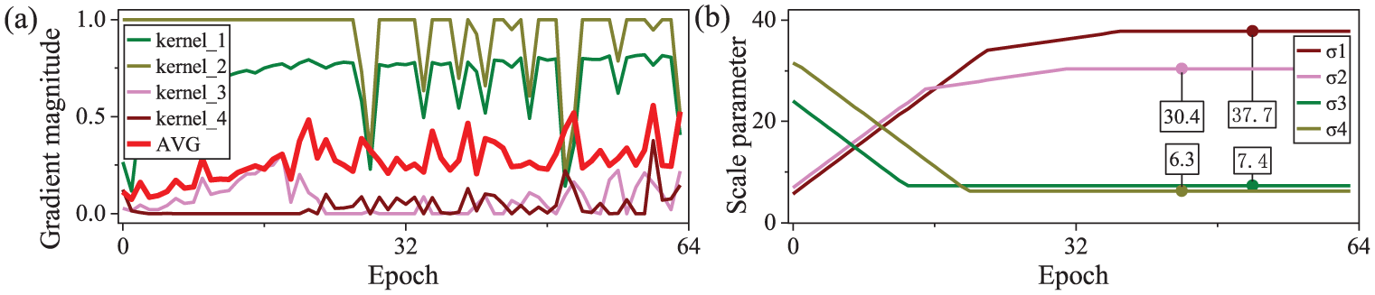
Dynamic modulation process of convolutional kernel gradient magnitude and Gaussian window scale parameter: (a) dynamic response of convolutional kernel gradient magnitude and (b) dynamic adjustment of Gaussian window scale parameter.

Based on the above frequency preference, adaptive adjustment of $\sigma$ is achieved via equation (16), ensuring accurate matching between the convolution kernel’s receptive field and feature frequencies.

$${\sigma }^{t+1}={\sigma }^t+\alpha ·\mathrm{sgn}(\overline{\mathrm{mag}}-{\Vert {\mathrm{mag}}_c\Vert }_2)$$

(16)

Where $\alpha$ is the adjustment coefficient, controlling the update step size of $\sigma$ ; $\mathrm{sgn}(·)$ is the sign function, determining the direction of increase or decrease of $\sigma$ . The specific adjustment logic of the above equation, as visualized in Figure 17(b; dynamic curve of the Gaussian window scale parameter), is detailed as follows.

First, when condition $\Vert {\mathrm{mag}}_c{\Vert }_2>\overline{\mathrm{mag}}$ is satisfied (the convolutional kernel is more sensitive to high-frequency features), it corresponds to $\mathrm{sgn}(\overline{\mathrm{mag}}-{\Vert {\mathrm{mag}}_c\Vert }_2)=-1$ ; subsequently, $\sigma$ decreases to reduce the receptive field, thereby enhancing the ability to capture high-frequency fluctuations. Second, when condition $\Vert {\mathrm{mag}}_c{\Vert }_2<\overline{\mathrm{mag}}$ is satisfied (the convolutional kernel is more sensitive to low-frequency features), it corresponds to sgn $(\overline{\mathrm{mag}}-{\Vert {\mathrm{mag}}_c\Vert }_2)=1$ ; accordingly, $\sigma$ increases to enlarge the receptive field, thus covering the wide-frequency domain distribution of low-frequency features.

Ultimately, through the synergistic effect of precise tracking via high-frequency narrow windows and stable coverage via low-frequency wide windows, this mechanism resolves the trade-off dilemma of traditional fixed-scale Gaussian windows, significantly improving the robustness of cross-working condition feature extraction.

• (2) Robustness verification of $\alpha$

The hyperparameter of the Gaussian window is the adjustment coefficient $\alpha$ , whose value affects the update speed of the scale parameter $\sigma$ , a too small value leads to adjustment lag while a too large value causes oscillation. To verify the model’s robustness to hyperparameter fluctuations, experiments are conducted with four sets of $\alpha$ values: 0.001, 0.01, 0.1, and 1, under the Ottawa scenario (B0 → B1, B2, B3, SNR = −15 dB). It can be seen from Figure 18 and Table 12 that different $\alpha$ values have a significant impact on both the adjustment process of $\sigma$ and model performance.

Figure 18.

Dynamic adjustment process of the scale parameter σ of dynamic Gaussian windows under different adjustment coefficients alpha: (a) $\alpha =0.001$ , (b) $\alpha =0.01$ , (c) $\alpha =0.1$ and (d) $\alpha =1$ .

Table 12.

Influence of different $\alpha$ on the Gaussian window scale parameter and model performance.

$\alpha$	Model performance F1	$\sigma$ regulates stability	$\alpha$ Robustness
0.001	95.43 ± 1.81	Stability, regulation lag	Better
0.01	97.12 ± 1.12	Stable and responsive quickly	Best
0.1	96.87 ± 2.34	Stable and responsive quickly	Better
1	56.25 ± 3.25	Fast response, large oscillation	Bad

First, when $\alpha =0.001$ , the adjustment of $\sigma$ is stable yet exhibits lag, failing to promptly adapt to changes in working conditions, with a corresponding model F1 of 95.43%.

Second, when $\alpha =0.01$ and $\alpha =0.1$ , $\sigma$ adjusts promptly without oscillation, achieving optimal working condition adaptability; the model’s F1 reach 97.12% and 96.87% respectively. Both values fall within the stable range of 95.43%–97.12%, with a maximum fluctuation of only 1.69%, fully demonstrating the model’s strong robustness to the hyperparameter $\alpha$ .

Finally, when $\alpha =1$ , severe oscillation of $\sigma$ leads to unstable feature extraction, and the model’s F1 plummets to 56.25%.

Considering both the stability of $\sigma$ adjustment and model classification accuracy, $\alpha =0.01$ is determined as the optimal hyperparameter value.

Comprehensive performance evaluation of WGS-CNN

To verify the practical performance of WGS-CNN in cross-working condition fault diagnosis, comprehensive evaluations proceed from three key dimensions: lightweight multi-dimensional performance focusing on resource consumption and basic diagnostic efficiency, strong noise robustness adapting to complex interference environments, and fault feature interpretability avoiding the black box problem and ensuring mechanism reliability. The evaluations are carried out using the CWRU stable working condition dataset and Ottawa variable working condition dataset as testbeds. Through comparative experiments with various mainstream improved CNN models, the comprehensive advantages of WGS-CNN in resource consumption, diagnostic performance, and mechanism reliability are ultimately verified.

Lightweight performance analysis

To more comprehensively evaluate the cross-operating condition diagnostic performance of WGS-CNN, this study selects five types of mainstream improved CNN frameworks to conduct comparative experiments, covering typical optimization directions in the field of cross-operating condition fault diagnosis. Specifically, they include: CNN based on Joint Loss Function (J-CNN), ³⁸ Joint Distribution Matching Embedding with Gaussian (JDME-G), ³⁹ Deep Convolutional Neural Networks with Wide First-layer Kernels (WDCNN), ⁴⁰ Convolutional Neural Networks and Long Short-Term Memory (CNN-LSTM), ²⁷ and Dual Path Convolution with Attention Mechanism and Bidirectional Gated Recurrent Unit (DCA-BiGRU). ⁴¹ The core characteristics and optimization logics of each model are as follows.

• (1) Joint Loss Optimization Direction: J-CNN achieves cross-working condition transfer learning of fault features through the joint constraint of classification loss + transfer loss, enhancing feature adaptability.

• (2) Distribution Matching Transfer Direction: JDME-G measures based on Extended Maximum Mean Discrepancy (EMMD) and matches the joint distribution from the source working condition to the target working condition via a mapping matrix, but limited by the signal stationarity assumption, it exhibits adaptability limitations in variable working condition scenarios.

• (3) Network Structure Improvement Direction: WDCNN enlarges the feature receptive field through the design of wide convolutional kernels, focusing on capturing global vibration features, but the model has relatively high parameter redundancy. CNN-LSTM and DCA-BiGRU integrate convolutional modules with temporal modules (LSTM/bidirectional GRU), attempting to improve adaptability to variable working conditions through temporal correlation, yet the temporal networks have a significantly higher demand for computing resources.

To ensure fair comparison, all models adopt consistent preprocessing protocols as detailed in Section 3.1: CWRU and Ottawa signals are unified to 2048 and 32,768 sampling points respectively, cross-working condition transfer uses the same source-target partition strategy, and all vibration signals are normalized to [0,1] via min-max scaling. We perform targeted hyperparameter tuning for each model based on its structure, using consistent optimization criteria: maximizing F1-score and minimizing convergence time. Common hyperparameters include a batch size of 64, Adam optimizer and early stopping with patience = 10, while model-specific parameters are optimized for their respective mechanisms.

All the aforementioned models are subjected to 10 repeated experiments on the CWRU (A0 → A1, A2, where A0 is the training set and A1–A2 are the test sets) and the Ottawa (B0 → B1, B2, B3, where B0 is the training set and B1–B3 are the test sets). In the following, the performance differences among the various models will be systematically compared from the four dimensions of lightweight performance, computational efficiency, diagnostic accuracy, and training speed in Table 13.

• (1) Significant lightweight advantages

Table 13.

Comparison of lightweight performance of different improved CNNs.

Model	Data sets	Parameter (K)	Floating-point computation (M)	AVG (M)	Size (KB)	Accuracy (%)	AVG (%)	Time (s)	AVG (s)
J-CNN	CWRU	8500.73	411.76	483.04	8563	100	99.17	47.37	132.88
								218.39
	Ottawa		554.32			98.33
JDME-G	CWRU	506.88	109.32	2166.7	549	100	97.98	26.14	81.34
								136.53
			4224.08			95.96
	Ottawa
WDCNN	CWRU	160.32	23.14	196.13	209	96.45	95.05	12.95	40.06
								67.17
	Ottawa		369.12			93.64
CNN-LSTM	CWRU	176.88	153.64	10462.44	203	91.52	94.47	48.18	329.91
								611.64
						97.42
	Ottawa		20,771.23
DCA-BiGRU	CWRU	604.18	747.23	6495.54	635	100	99.07	33.83	263.28
								492.72
						98.13
	Ottawa		12,243.85
WGS-CNN	CWRU	8.73	4.19	35.68	26	100	99.86	15.37	33.56
								51.78
	Ottawa		67.16			99.72

In the dimension of model lightweighting, the parameter count of WGS-CNN is only 8.73 K, accounting for 0.11%, 1.72%, 5.44%, 4.93%, and 1.44% of that of J-CNN, JDME-G, WDCNN, CNN-LSTM, and DCA-BiGRU respectively. Parameter redundancy is significantly compressed. Correspondingly, its model size is merely 26 KB, which is 0.31% of J-CNN, 4.74% of JDME-G, 12.44% of WDCNN, 12.81% of CNN-LSTM, and 4.09% of DCA-BiGRU. Such extreme lightweight characteristics endow it with significant application advantages in computing resource-constrained scenarios such as industrial embedded devices and portable monitoring terminals, solving the pain points of traditional deep learning models: large size and difficulty in deployment.

• (2) Outstanding computational efficiency

Building on its lightweight advantage, WGS-CNN also delivers impressive computational efficiency: its average floating-point operations (FLOPs) stand at 35.68M, representing only 7.38% of J-CNN, 1.65% of JDME-G, 18.19% of WDCNN, 0.34% of CNN-LSTM, and 0.55% of DCA-BiGRU. This advantage stems from two layers of design logic.

• (1) The highly simplified design of the single-layer convolutional architecture can directly eliminate computational redundancy caused by repeated iterations of multi-layer networks.

• (2) The learnable window function can dynamically focus on fault feature regions, reducing invalid computations on irrelevant noise, thereby significantly enhancing the model’s real-time diagnostic capability and meeting the demand for low-latency diagnosis in scenarios such as embedded devices and portable monitoring terminals.

• (3) Leading diagnostic accuracy

In the dimension of diagnostic accuracy, WGS-CNN still maintains a leading position: its average accuracy on two datasets reaches 99.86%. Though only slightly higher than that of J-CNN (99.17%) and DCA-BiGRU (99.07%), it is significantly superior to JDME-G (97.98%), WDCNN (95.05%), and CNN-LSTM (94.47%). These results indicate that WGS-CNN does not sacrifice diagnostic accuracy while controlling model complexity, achieving a balance between lightweighting and high accuracy.

• (4) Efficient training Speed

WGS-CNN also exhibits outstanding training efficiency, with an average convergence time of only 33.56 s, representing 25.26% of that of J-CNN, 41.26% of JDME-G, 83.77% of WDCNN, 10.17% of CNN-LSTM, and 12.74% of DCA-BiGRU respectively. This high-efficiency performance stems from the synergistic effect of three mechanisms.

• (1) Wavelet initialization injects prior knowledge of time-frequency domain localization into convolutional kernels, reducing the time spent on random parameter search.

• (2) The learnable window function accelerates the convergence of parameters toward the direction adapted to fault features through dynamic scale adjustment.

• (3) The gradient optimization characteristics of square mapping fundamentally avoid the problems of neuron death and training stagnation.

To further verify the diagnostic performance of WGS-CNN, a comparative analysis of various models was conducted on the CWRU and Ottawa datasets based on four metrics: Accuracy (Acc), Precision (Pre), Recall (Rec), and F1-score (F1; as shown in Figure 19). The results indicate that on the CWRU dataset, except for WDCNN and CNN-LSTM, the four metrics of all other models reach 100%; on the other hand, on the Ottawa dataset, the Acc, Pre, and F1 metrics of WGS-CNN are higher than those of the comparative models. Especially in complex variable working condition scenarios, its stable capability to capture cross-working-condition fault features is more prominent.

Figure 19.

Comparison of diagnostic performance of different improved CNN: (a) CWRU and (b) Ottawa.

Overall, through systematic optimizations including wavelet initialization for feature anchoring, learnable window for dynamic alignment, square mapping for energy enhancement, and single-layer architecture for redundancy reduction, WGS-CNN has achieved a threefold breakthrough of lightweight, high efficiency, and high precision in cross-working-condition diagnosis. Its performance advantages are reflected not only in low resource consumption such as parameter count and computational complexity (the single-layer architecture avoids iterative redundancy, and the learnable window reduces invalid computations) but also in diagnostic stability and high precision under complex working conditions (wavelet initialization guides feature learning, and square mapping ensures stable training). Ultimately, it achieves a balance between low resource consumption and excellent diagnostic performance.

Anti-noise performance analysis

To more accurately evaluate the cross-working-condition diagnostic robustness of WGS-CNN in complex noisy environments, this section conducts comparative experiments on anti-noise performance with differentiated signal-to-noise ratio (SNR) levels according to the characteristics of different datasets: five levels (10, 5, 0, −5, −10 dB) are selected for the CWRU stable working condition dataset; five levels (15, 5, 0, −5, −15 dB) are chosen for the Ottawa variable working condition dataset (covering a wider noise range to match the complex interference in variable working condition scenarios). The experiment simulates real interference by adding additive white Gaussian noise proportional to the amplitude of clean signals. ⁴² The comparative design is divided into two categories: first, horizontal comparison with different traditional anti-noise strategies on the CWRU dataset; second, vertical comparison with various mainstream improved CNN models on the Ottawa dataset, with detailed analyses as follows.

• (1) Horizontal comparison based on CWRU

To verify the adaptive anti-noise performance of WGS-CNN, two comparative models, WD-CNN (wavelet denoising + basic CNN) and WF-CNN (Wiener filtering + basic CNN), were constructed in ablation experiments by replacing its dynamic anti-noise mechanism with traditional preprocessing methods. Cross-working-condition anti-noise experiments were then conducted on the CWRU dataset.

Three cross-working-condition scenarios were set up (with one of them as the source working condition and the rest as the target working condition): A0 → A1, A2; A1 → A0, A2; and A2 → A0, A1. The focus was on analyzing the changes in F1-score of the three models within the noise intensity range from 10 dB (weak noise) to −10 dB (strong noise), and the results are shown in Figure 20. It can be seen from the figure that WGS-CNN exhibits superior anti-noise robustness across the entire noise range, with particularly prominent advantages under the strong noise of −10 dB: the F1 values reach 92.0% in the A0 → A1, A2 scenario, 91.2% in the A1 → A0, A2 scenario, and 87.2% in the A2 → A0, A1 scenario, all significantly higher than those of WD-CNN and WF-CNN.

Figure 20.

Anti-noise performance of different improved CNN models based on CWRU: (a) A0 → A1, A2, (b) A1 → A0, A2 and (c) A2 → A0, A1.

Both types of traditional models have significant limitations: Although WF-CNN adopts adaptive Wiener filtering with a sliding window for real-time estimation of the local statistical characteristics of signals, its fixed window struggles to adapt to abrupt changes in signal frequency and noise intensity under cross-working conditions, often leading to incomplete noise suppression or loss of effective features; on the other hand, WD-CNN relies on a fixed wavelet threshold and fails to dynamically match the noise distribution during working condition changes, resulting in insufficient flexibility.

The excellent performance of WGS-CNN stems from the synergy of three dynamic mechanisms.

• (1) Wavelet initialization aligns with the frequency-domain characteristics of vibration signals, providing a reasonable starting point for parameter learning while initially suppressing noise in the central region of convolution kernels.

• (2) The dynamic-scale Gaussian window can adjust focusing range with working conditions, accurately locking onto local effective features, and also weakening high-frequency noise through its smoothing property.

• (3) Square activation enhances the main peak features critical for classification, and realizes real-time optimization of the Gaussian window scale and convolution kernel weights through gradient backpropagation, forming a “feature enhancement-parameter optimization” closed loop.

This mechanism avoids the rigid limitations of traditional models, ultimately achieving performance far superior to the two comparative models under cross-working-condition strong noise.

• (2) Longitudinal comparison based on Ottawa

To verify the anti-noise superiority of WGS-CNN, a vertical comparison was conducted between WGS-CNN and mainstream improved CNN models (WDCNN, J-CNN, JDME-G, CNN-LSTM, DCA-BiGRU) on the Ottawa dataset, with a focus on testing four cross-working-condition transfer scenarios (B0 → B1, B2, B3; B1 → B0, B2, B3; B2 → B0, B1, B3; B3 → B0, B1, B2). The results (shown in Figure 21) indicate that WGS-CNN exhibits outstanding performance under a wide noise range of 15 to −15 dB and superimposed interference of variable rotational speeds. Under the strong noise scenario (−15 dB), the F1 values reach 97.1% in the B0 → B1, B2, B3 scenario, 91.5% in B1 → B0, B2, B3, 90.6% in B2 → B0, B1, B3, and 87.8% in B3 → B0, B1, B2, all outperforming the comparative models.

Figure 21.

Anti-noise performance of different improved CNN models based on Ottawa: (a) B0 → B1,B2,B3, (b) B1 → B0,B2,B3, (c) B2 → B0,B1,B3 and (d) B3 → B0,B1,B2.

Comparative models have obvious limitations in this scenario: Although WDCNN uses wide convolution kernels to capture global features, when strong noise is superimposed with variable rotational speeds, it struggles to distinguish between noise and effective signals and tends to incorporate high-frequency noise; J-CNN (joint loss) and JDME-G (Gaussian distribution matching) focus on transfer learning but lack targeted anti-noise designs. Moreover, the Gaussian assumption of JDME-G fails as variable rotational speeds destroy the stationarity of signals, resulting in distribution matching deviations; CNN-LSTM and DCA-BiGRU rely on temporal modules to capture rotational speed correlations, but temporal networks are sensitive to strong noise and have not optimized frequency-domain feature extraction under variable rotational speeds, thus tending to be disturbed by redundant information.

Consistent with its performance in the CWRU dataset, WGS-CNN’s advantages stem from its dynamic collaborative anti-noise and feature enhancement mechanism. This mechanism addresses the static structure or single-dimensional optimization defects of the comparative models, thus maintaining excellent performance across the entire noise range, especially under strong noise.

Interpretability analysis

To further verify WGS-CNN’s ability to capture fault features, this section takes the Ottawa dataset (under a strong noise environment, SNR = −15; B0 → B1, B2, B3 scenario) as the research object. It compares the convolution kernel morphologies and time-frequency feature maps of different improved CNN models through visual analysis, thereby revealing the source of advantages in WGS-CNN’s feature representation capability.

• (1) Morphology analysis of convolutional kernel

Convolution kernels are the feature extraction units of the model, and their morphologies directly determines the accuracy of feature capture. Figure 22 shows the learned convolution kernel morphologies of various models on the Ottawa dataset (B0 → B1, B2, B3) under SNR = −15. The main differences among the models are specifically reflected in their ability to maintain time-frequency localization characteristics, with detailed analyses as follows.

Figure 22.

Comparison of convolutional kernel waveforms learned by different improved CNNs: (a) J-CNN, (b) JDME-G,(c) WDCNN, (d) CNN-LSTM, (e) DCA-BiGRU and (f) WGS-CNN.

WDCNN, CNN-LSTM, and DCA-BiGRU have disorderly convolution kernel waveforms, that barely possess time-domain localization characteristics, and cannot effectively focus on transient fault impact signals, making such models prone to losing the learning direction of fault features under strong noise. J-CNN and JDME-G perform slightly better but still have significant drawbacks, their convolution kernels are significantly affected by noise interference, with severe waveform fluctuations and distinct high-frequency burrs, which means their learning processes are dominated by noise, failing to stably capture effective fault features, and resulting in insufficient robustness in feature extraction. In contrast, WGS-CNN’s convolution kernels exhibit a regular morphology with a compact middle and gentle sides, the middle part retains the time-frequency localization characteristics of wavelets, to accurately focus on high-frequency fault impacts, while the two sides show low-frequency sinusoidal vibrations, to cover stable features in a wide frequency domain. This characteristic stems from the synergy of two mechanisms, the dynamic constraints of the Gaussian window enable the convolution kernels to retain the initial wavelet morphology, avoiding excessive deviation from prior knowledge, and the square nonlinear mapping suppresses high-frequency and low-amplitude noise, amplifying the energy gap between effective features and noise, thus ultimately forming convolution kernel characteristics that focus on key features and filter interference.

In summary, the morphological differences of convolution kernels fully reflect the gap in feature capture capabilities among models. WGS-CNN’s regular and noise-resistant kernel morphology, shaped by the dual mechanism, lays a solid foundation for its superior feature representation under strong noise, which is incomparable to the comparative models.

• (2) Time-frequency analysis of feature maps

The morphological differences of convolution kernels directly affect feature extraction performance. The following section further analyzes the actual fault feature extraction capabilities of various models through time-frequency domain feature maps, with the results shown in Figure 23.

Figure 23.

Comparison of time-frequency domain features of B0-IR learned by different improved CNNs: (a) clean raw, (b) noisy raw, (c) J-CNN, (d) JDME-G, (e) WDCNN, (f) CNN-LSTM, (g) DCA-BiGRU and (h) WGS-CNN.

Figure 23 presents the B0-IR time-frequency diagrams extracted by different improved CNN models on the Ottawa dataset (B0 → B1, B2, B3) under SNR = −15. It should be noted that under the B0 working condition, the IR rotational speed increases from 12.5 to 27.8 Hz, and the IR samples selected in this experiment are close to the initial rotational frequency of 12.5 Hz. According to the fault mechanism, the theoretical characteristic frequencies of IR in this scenario are as follows: fundamental frequency of 67.9 Hz (12.5 Hz × 5.432, where 5.432 is the fixed multiple of the fault frequency to the rotational frequency), second harmonic of 135.8 Hz (67.9 Hz × 2), third harmonic of 203.7 Hz (67.9 Hz × 3), as well as sidebands of 42.9 and 92.9 Hz (combined frequencies of the fundamental frequency and rotational frequency).

Against the scenario where strong noise obscures the original fault signals, the differences in feature extraction capabilities among various models are significant.

• (1) J-CNN, WDCNN, CNN-LSTM, and DCA-BiGRU can only capture some discrete frequencies such as J-CNN learns 92.9 Hz and WDCNN learns 160.8 Hz, with blurred features and obvious noise interference, failing to fully cover the theoretical characteristic frequencies.

• (2) Although JDME-G can learn more frequency components, the clarity of fault features is low, the proportion of noise energy in the time-frequency diagram is high, and key harmonics (e.g. 135.8 Hz) are obscured.

• (3) In sharp contrast to the aforementioned models, WGS-CNN’s time-frequency diagram exhibits significant advantages: it not only clearly captures the fundamental frequency of 67.9 Hz and the second harmonic of 135.8 Hz but also fully retains the sidebands of 42.9 and 92.9 Hz, with concentrated feature energy, strong continuity, and effectively suppressed noise. This result verifies its collaborative mechanism of wavelet initialization anchoring features, learnable window function dynamically focusing, and square mapping enhancing energy. Even under strong noise, it can still stably extract the full-frequency-domain fault features, especially fully retaining the inherent proportional relationship between harmonics and the fundamental frequency, thereby providing reliable feature support for cross-working-condition fault diagnosis.

In summary, WGS-CNN exhibits stronger fault feature representation capability through the optimization of convolution kernel morphology and high-quality extraction of feature maps. This capability stems from the systematic design of time-frequency prior injection, dynamic scale adaptation, and energy contrast enhancement, enabling it to accurately capture the essential features of faults even in strong noise and cross-working-condition scenarios.

Conclusion

To address multiple faults and fault severity detection under complex operating conditions, this work proposes WGS-CNN, a novel framework that transcends the fragmented component stacking of conventional wavelet-CNN hybrids, such as WD-CNN and WaveNet. The model directly overcomes three critical limitations of existing methods: fixed wavelet kernels that hinder adaptive learning, static Gaussian filtering with poor cross-condition adaptability, and ReLu activation that suppresses weak fault features. WGS-CNN integrates three synergistic mechanism-level innovations, forming a closed-loop optimization encompassing prior injection, dynamic adaptation, and feature enhancement. Multi-scale wavelet initialization with retained backpropagation fuses time-frequency prior knowledge with adaptive learning; a learnable Gaussian window module dynamically constrains convolutional kernels to align with time-varying fault features; and square function activation embeds power spectrum enhancement into end-to-end training to strengthen weak signals. This design fundamentally resolves the static working modes of traditional wavelet-CNNs and advances wavelet-deep learning fusion for complex-condition fault diagnosis.

Experimental results demonstrate WGS-CNN’s excellent comprehensive performance in rotating machinery fault diagnosis. The model exhibits robust cross-condition adaptability, scenario-stable operation, and superior capabilities compared to traditional CNNs. Its high universality enables multi-signal adaptation with minimal modifications, supporting acoustic emission signals paired with Morlet and narrow windows, motor current signals integrated with notch filters and Haar wavelets, and multimodal data processed via multi-branch attention mechanisms.

Collaborative innovation of fault-targeted initialization, dynamic window constraint, and weak feature enhancement significantly boosts CNNs’ diagnostic capability in complex industrial scenarios. WGS-CNN thus provides a high-accuracy, lightweight, and robust-generalization paradigm for rotating machinery fault diagnosis. Future work will extend the lightweight and cross-condition adaptable framework to data decentralization scenarios using federated learning, addressing key challenges in industrial fault diagnosis, such as data privacy protection and high transmission costs. ⁴³