Sage Journals: Discover world-class research

Abstract

This study proposes a coupled framework integrating wheel wear, track irregularities, and frozen conditions, while incorporating track irregularity amplitudes and ice mass into the analysis. The impact of speed and track irregularity amplitude at different wheel wear stages on comfort is evaluated using a comfort index. The study found that as the track irregularity amplitude increases, the standard wheel profile becomes more sensitive to such changes than the worn wheel profile. To assess safety, we analyzed the effect of track irregularity amplitude and curve radius on wheel lateral forces and wheelset lateral displacement. We found that curves with a radius of 400 m are hazardous curves. The study demonstrates that the track irregularity amplitude coefficient continuously decreases as wheel wear increases, correlating with a higher risk of derailment. Under frozen condition, the wheel profile at 50,000 km demonstrates the best overall vehicle performance. However, when track irregularity amplitudes reach the range of −3 to 3 mm, vehicle safety indicators exceed the permissible critical thresholds. This method provides theoretical guidance for wheel optimization and rail grinding to enhance the service life of railway components.

Keywords

wheel wear high-speed train derailment track irregularity amplitude coefficient frozen conditions

Introduction

Track irregularities and wheel wear are two key factors affecting the dynamic performance of high-speed trains. Track irregularities alter the wheel–rail contact geometry and accelerate uneven wheel wear, while wheel wear can further amplify the dynamic responses induced by track excitations. Their coupled effects jointly influence the running stability and safety during long-term service. Therefore, a combined investigation of track irregularities and wheel wear is essential for understanding the performance evolution of high-speed trains and optimizing maintenance strategies. In response to this problem, numerous scholars have conducted research on vehicle dynamics under different wear patterns. Barke and Chiu¹ found that as the velocity of vehicle increases, the extent of wheel polygons expands, leading to noise production, decreased ride comfort, component damage, and track deterioration. Based on this, Peng et al.² have identified several patterns in the variation of vehicle polygons and set out conditions that trigger the progression of wheel polygon wear. In addition, Pradhan et al.³ evaluated the impact of flange and tread wear on dynamic characteristics such as safety, thereby justifying the necessity of wheel maintenance. Hou et al.⁴ discovered that the formation of hollow wear on wheels leads to a gradual degradation of vehicle dynamic performance. Zhu et al.⁵ synthesized previous research to investigate the effects of flange and tread wear on vehicle dynamics under different track conditions. The study found that wheels with tread wear exhibit better performance on curved tracks compared to those with flange wear. By investigating the influence of actual wheel wear on vehicle dynamics, Li et al.⁶ found that a larger diameter of the outer wheel on curves improves performance, and that the rate of performance degradation slows down as wear progresses. Wheel wear alters the wheel profile. An important factor in how wheels and rails interact is the profile. It significantly affects the location of the wheel–rail contact, consequently impacting the stability of train operation.^7–10 Many researchers investigate wheel wear using field measurements, simulation predictions, and scaling tests. A substantial amount of research is dedicated to examining how wheel wear affects vehicle operational performance.¹¹

Furthermore, track irregularities also affect the wheel–rail interaction. Choi et al.¹² investigated the impact of track irregularities on vehicle operation. The results indicated that track alignment has a significant effect on safety, while longitudinal level irregularities exhibit minimal influence. Subsequently, Liu et al.¹³ investigated the combined effects of operating speed and track irregularities on vehicle behavior, with a systematic evaluation of ride comfort. Xin et al.¹⁴ investigated the influence of long-wavelength track irregularities on ride comfort and running stability, with results demonstrating a significant impact. Chang et al.¹⁵ investigated the impact of track irregularities in switch zones on vehicle operation. The results indicate that the influence of track irregularities on vehicle performance is primarily concentrated within frequency ranges below 200, 50, and 20 Hz. Bosso et al.¹⁶ investigated the influence of track irregularities on railway vehicle dynamics and proposed a sensitivity analysis method to detect safety-critical track irregularities.

Our research focuses on the entire line, where certain cold sections may experience frozen conditions. Numerous scholars have conducted studies on vehicle dynamics under such frozen conditions. Hong et al.¹⁷ investigated the influence of snow particle diameter on vehicle dynamics and found that it significantly affects train speed. Teng et al.¹⁸ studied the impact of low-temperature conditions on vehicle dynamics and found that the lateral ride quality of vehicles deteriorates significantly under polar temperature conditions. Gao et al.¹⁹ discovered that snow accumulation on bogies can severely compromise vehicle safety, stability, and ride comfort. Song and Luo²⁰ investigated vehicle dynamics at −40 °C conditions. The research showed that wheel–rail interaction forces increase significantly under extreme cold temperatures, substantially impacting ride comfort and operational safety. Further research by Luo et al.²¹ examined vehicle dynamics at −20 °C demonstrated that snow accumulation severely compromises suspension functionality, leading to substantial deterioration in dynamic performance.

Previous studies have primarily focused on specific types of track irregularities, with limited investigation into the effect of irregularity amplitudes. Research under frozen conditions has also overlooked the influence of ice mass. Furthermore, no existing framework has yet integrated wheel wear, track irregularities, and frozen conditions into a coupled analysis. Our study addresses these gaps by incorporating track irregularity amplitudes and ice mass, while establishing a comprehensive coupled model that simultaneously accounts for wheel wear, track irregularities, and frozen conditions. This enables vehicle dynamic analysis of the entire railway line. The differences in the impact of track irregularity amplitude on the inner and outer rails in curves are analyzed, and the critical track irregularity amplitude is examined. Furthermore, the effects of track irregularities and wheel wear on vehicle performance were analyzed under different frozen conditions with varying ice masses. Finally, a comprehensive consideration is made to select appropriate wheel profiles and grind rails to ensure both economic efficiency and safety.

Wheel–rail coupling dynamics model

Modeling and analysis

Based on the CR400BF high-speed train, a high-speed vehicle model was developed in Simpack, as shown in Figure 1. The model adopts a standard 60 N rail profile with a gauge of 1.435 m and consists of one carbody, two bogies, four wheelsets, eight axle boxes, and steel rails. For computational efficiency, all components are modeled as rigid bodies. The suspension system is represented by both primary and secondary suspensions. Each wheelset, bogie, and the carbody possesses six degrees of freedom, including vertical, lateral, longitudinal, roll, pitch, and yaw motions. Each axle box is constrained to a single vertical degree of freedom, yielding a total of 50 degrees of freedom for the entire CR400BF train model. In the suspension system, nonlinear characteristics are adopted for the lateral stop and the secondary lateral damper. Table 1 below summarizes in detail the principal parameters of train model, all of which are derived from measured data. Rigid bodies serve as a simplification of the model and cannot fully replicate real-world conditions. Therefore, validation is necessary to ensure the accuracy of the results. This study focuses on the effect of temperature on the suspension system and does not consider temperature-dependent friction models.

Figure 1.

CR400BF high-speed train model.

Table 1.

The principal parameters of train model.

Parameter name	Value	Unit
Mass of carbody	42,000	kg
Inertia moment of carbody (x/y/z)	104,700/1,971,000/1,938,000	kg/m²
Mass of bogie	2439	kg
Inertia moment of bogie (x/y/z)	1846/1205/2792	kg/m²
Mass of wheelset	1713	kg
Inertia moment of wheelset (x/y/z)	1045/111/1050	kg/m²
Longitudinal stiffness of primary suspension	919,800	N/m
Lateral stiffness of primary suspension	919,800	N/m
Vertical stiffness of primary suspension	886,500	N/m
Longitudinal stiffness of air-spring	12,400	N/m
Lateral stiffness of air-spring	12,400	N/m
Vertical stiffness of air-spring	18,200	N/m
Longitudinal damping of air-spring	8400	N·s/m
Lateral damping of air-spring	8400	N·s/m
Vertical damping of air-spring	3000	N·s/m

Figure 2 shows the comparison between measured and simulated carbody accelerations and acceleration frequency spectrum. According to the measured carbody acceleration and our simulation results, the lateral acceleration fluctuates between −0.15 and 0.15 m/s², showing good agreement with the measured data in overall trend. The vertical acceleration ranges from −0.12 to 0.20 m/s², with both magnitude and variation trend consistent with the experimental measurements. Figure 2(b) shows dominant lateral frequencies of 0.65 Hz (measured) and 0.67 Hz (simulated), and vertical frequencies of 1.09 Hz (measured) and 1.1 Hz (simulated). The correlation coefficients between vehicle body acceleration and frequency spectra all exceed 0.8, with overall errors remaining within 20%. The overall spectral densities also show good agreement. The correlation coefficients between vehicle body acceleration and frequency spectra all exceed 0.8, with the average error remaining within 10%. Based on our previous research,²² the high-speed train model has been validated, demonstrating good agreement between predicted and measured wear. This model can be applied to the research presented in this paper.

Figure 2.

Comparison of lateral and vertical carbody accelerations (a) and acceleration frequency spectrum (b).

Model of wheel–rail contact interactions

The wheel–rail contact model adopts the LMB10 wheel profile and the 60 N rail profile. The track parameters, representative of the Beijing–Shanghai high-speed line, include a gauge of 1435 mm and a rail cant of 1:40. The wheelset has a wheel diameter of 0.92 m and a track gauge of 1493 mm. All wheel–rail contact parameters are automatically calculated by Simpack. The wheel–rail interface refers to the region where the steel wheel meets the steel rail (a small elliptical contact patch typically about 1 cm² in area). The contact point is primarily located on the wheel tread but can shift toward the flange under certain operating conditions. Over time, repeated contact induces wear on both the flange and the tread, gradually resulting in the formation of concave profiles in these regions.

The wheel–rail contact interaction poses a significant challenge in vehicle dynamics, as it directly influences the operational performance of high-speed trains. In this study, wheel profiles of CR400BF trains operating on the Beijing–Shanghai line are analyzed, with measurements taken every 50,000 km over a total mileage of 206,000 km. Subsequently, the spatial distribution of the wheel–rail contact regions is examined.

Figure 3 illustrates the points distribution between the LMB10 profile and the standard 60 N rail, where variables a, b, c, d, and e represent contact distributions at mileages of 0, 50,000, 100,000, 150,000, and 200,000 km, respectively. The blue lines connecting the wheel and the rail indicate the contact conditions under different degrees of lateral displacement of the wheelset. The wheel–rail geometric contact is calculated using a multi-point contact algorithm, and the normal and tangential forces of wheel–rail contact are computed based on the Hertz theory and Kalker’s FASTSIM model.^23,24 Hertz and Fastsim are used to calculate creep relationships within elliptical contact patches rather than non-elliptical ones. However, as this paper does not focus on the detailed stress distribution inside the contact patch, Hertz and Fastsim strike a balance between computational speed and result accuracy.

Figure 3.

Wheel–rail contact distribution at different mileages (x-axis is the lateral position of the wheel and rail (m), y-axis is the vertical position of the wheel and rail (m), a, b, c, d, and e represent the wheel-rail contact distributions at 0, 50,000, 100,000, 150,000, and 200,000 km, respectively.).

As shown in Figure 3, the interaction between the LMB10 wheel profile and the 60 N rail primarily occurs at the flange and tread, with a significant concentration on the tread. As mileage increases, the contact points become more dispersed along the tread–rail interface, while the distribution near the wheel flange remains relatively unchanged. The expanded contact range on the tread leads to an uneven distribution of contact forces between the wheel and rail, adversely affecting vehicle dynamics. The contact behavior calculated from the measured wheel–rail profiles indicates that wear can degrade dynamic performance, providing a foundation for subsequent dynamic simulations.

Selection and scaling of track irregularities

Based on long-distance track irregularity measurements, a section with low-interference irregularities was identified in this study. As the concept of low track irregularity has been well documented in previous research,²⁵ this section was selected as the starting point for the analysis. The measured low-interference track irregularities from the Beijing–Shanghai line are shown in Figure 4. The measured lateral and vertical irregularities over a 470 km section indicate that, aside from a few locations with relatively large amplitudes, the overall amplitude range remains within −2to 2 mm. Therefore, the segment from 775 to 785 km was adopted for the simulations, as it sufficiently covers the mileage required for all simulation conditions. As shown in Figure 4, the irregularity amplitudes in both the lateral and vertical directions are approximately within the range of −2 to 2 mm.

Figure 4.

Left lateral and vertical track irregularities (a) and right lateral and vertical track irregularities (b).

However, in actual operation, the severity of track irregularities can vary significantly depending on track conditions, maintenance status, and accumulated service mileage. To account for this variability and to investigate the vehicle’s dynamic response under different track quality levels, several representative irregularity amplitudes were considered in the simulations. We have established the track irregularity amplitude range of −2 to 2 mm as the baseline, an amplitude scaling coefficient is introduced to modify the amplitude of the track irregularity. This amplitude coefficient is used to scale the entire irregularity function. Yu et al.²⁵ indicates that the high-amplitude range of track irregularities on the Beijing–Shanghai line is between −4 and 4 mm. To explore scenarios for extending rail service life, we discuss conditions with higher amplitudes. Therefore, we set the maximum amplitude coefficient to 3.0, corresponding to an amplitude range of −6 to 6 mm. Amplitude coefficients of 0.5, 1.0, 1.5, 2, 2.5, and 3.0 correspond to amplitude ranges of −1 to 1, −2 to 2, −3 to 3, −4 to 4, −5 to 5, and −6 to 6 mm, respectively.

Wheel wear analysis within one reprofiling cycle

Measured wheel wear evolution

From 2017 to 2018, wheel profiles on the Beijing–Shanghai line were inspected at intervals of 50,000 km. The wheel profiles were measured using a MiniProf, which is fixed on the wheel flange and records the wheel profile along the axial direction with a 0.25 mm sampling interval and a measurement uncertainty of ±0.001 mm. Figure 5 presents the measured wheel wear and the corresponding variations in wheel profiles obtained through instrumental measurements. Both wheels exhibited nearly identical wear patterns, and all wear values were referenced to the standard profile. As shown in Figure 5, the left wheel flange experienced greater wear than the right wheel flange. An investigation into the curvature characteristics of the Beijing–Shanghai line revealed that the total length of curved sections is 491.69 km, comprising 266.95 km of left-hand curves and 224.74 km of right-hand curves, accounting for ∼54% and 46% of the total curved length, respectively. The predominance of left-hand curves increases the likelihood of the left wheel flange contacting the rail, leading to greater flange wear. The equivalent conicity range for the left wheel under different wear conditions is 0.18–0.24, whereas that for the right wheel is 0.15–0.22. All conicity values remain below the limit of 0.4, confirming that the wheels remain within their effective service life.

Figure 5.

The measured wheel shape and wear in the first wheelset. (a) Left wheel and (b) right wheel, x-axis: wheel lateral position distribution (m), left wheel, y-axis: wheel vertical position distribution (m), and right wheel, y-axis: wear depth (mm).

Figure 5(a) displays that the flange wear at the left wheel flange roughly occurs between −32 and −42 mm, and the tread wear occurs between −31 and 47 mm. Figure 5(b) suggests that the wear at the right wheel flange is roughly between −31 and −43 mm, and the wear at the tread is between −29 and 48 mm. Both figures demonstrate that the maximum wear value is located at the flange. With increasing wear, depressions form on the wheel tread and flange. As illustrated in Figure 3, the depression on the wheel tread expands the wheel–rail contact zone, which may shift the contact position toward the flange and consequently degrade vehicle dynamic performance.

Analysis of measured wear depth

Figure 6 depicts the relationship between measured wheel wear and mileage for sixteen wheels from the first and second vehicles, illustrating the maximum, quartile, median, mean, and minimum wear depths. The mileage ranges from 33,000 to 206,000 km.

Figure 6.

(a) Flange and (b) tread position of the wheel during the reprofiling cycle wear.

Figure 6(a) demonstrates that the average wear at the flange increases linearly with mileage. By comparing with Figure 6(b), it is apparent that the tread has less mean wear than the flange. The wear amount was calculated from measured wheel–rail profiles. Then, the wear rate was determined by taking the ratio of the total wear amount accumulated over 0 to 200,000 km to the total distance traveled. The mean rate of wear at the tread is ∼0.049 mm/10,000 km, with the maximum wear depth reaching about 1.13 mm. In contrast, the average wear rate at the flange is ∼0.12 mm/10,000 km, with a maximum wear depth of about 3.38 mm. According to the median values in Figure 6, significant differences exist between the flange and tread across the sixteen wheels, with the median distribution at the flange notably greater than that at the tread. The multi-wheel wear analysis underscores the universal phenomenon of the dominance of flange wear, thereby providing support for the single-wheel simulation study.

Impact of wheel wear and track irregularity on dynamics

Under straight-track conditions, the analysis framework is structured around ride comfort index, while on curved sections the focus shifts to safety-critical parameters including derailment coefficient, wheel unloading rate, lateral force, and wheelset lateral displacement. Specific track parameters are detailed in Table 2. The speed selection is based on typical operating speeds derived from long-term tracking data.

Table 2.

Track parameters for vehicle dynamics calculation.

Line type	Superelevation (mm)	Operation speed (km/h)
Straight line	–	200/250/300/350
R400 m	100	120
R800 m	160	120
R3500 m	125	200
R5500 m	175	300

Ride comfort analysis

In this study, the Sperling index is employed to evaluate the smoothness of the vehicle’s wheel profiles under varying degrees of wear. The low track irregularities of the Beijing–Shanghai line are incorporated into a linear track model at the specified time.

Figure 7(a) presents the lateral and vertical frequency-weighting curves for the comfort index at specific frequencies. Figure 7(b) shows the corresponding lateral and vertical accelerations of the carbody. These acceleration signals were filtered using the aforementioned weighting curves to calculate the Sperling index.

Figure 7.

Weighting curve (a) and carbody acceleration (b).

As illustrated in Figure 8, the stability index increases with speed. At a mileage of 50,000 km, raising the velocity from 250 to 300 km/h results in a 5.1% increase in the lateral Sperling index, whereas the vertical Sperling index shows only a slight increase. Figure 8(a) further demonstrates that the lateral index exhibits an upward trend with accumulating mileage at 350 km/h, the lateral index increases by 8.7% as mileage grows from 0 to 200,000 km. Similarly, Figure 8(b) indicates a modest 2% increase in the vertical index over the same mileage at this speed.

Figure 8.

Sperling index at different operation distance and velocities (x-axis is the operation distance (×10,000 km), y-axis is velocity (km/h), z-axis is sperling index, a and b represent the lateral and vertical sperling index, respectively, the limited value is 3.00).

The results indicate that with increasing speed and wear, the lateral index rises significantly while the vertical index remains almost unchanged, leading to a continuous deterioration of vehicle stability. According to the Code for Evaluation and Test Evaluation of Dynamic Properties of Locomotives and Vehicles,²⁶ passenger car ride stability is evaluated as shown in Table 3. Through hunting stability simulation, the critical speeds obtained for the worn wheel profiles at 0, 50,000, 100,000, 150,000, and 200,000 km are 823, 720, 640, 618, and 592 km/h, respectively. As the operating mileage increases, the critical speed decreases but still exceeds the maximum test speed of 420 km/h. Comparative analysis with Figure 8 demonstrates that the vehicle exhibits excellent stability performance.

Table 3.

Stability index of passenger vehicle.

Stability level	Riding index	Evaluation
1	W ≤ 2.5	Excellent
2	2.5 < W ≤ 2.75	Good
3	2.75 < W ≤ 3	Qualified

Figure 9 illustrates the variations of the lateral and vertical Sperling indices with respect to track irregularity amplitude and operation distance. The lateral index increases from about 0.7 to 2.8 as the amplitude coefficient rises from 0 to 3.0, representing nearly a 300% growth, while the vertical index only rises from 1.0 to 1.5, indicating much lower sensitivity. The influence of irregularity amplitude is more evident during the early wear stage (0–5 × 10⁴ km) and tends to stabilize after 15 × 10⁴ km. Notably, when the amplitude coefficient reaches 3.0 at 0 km, the lateral comfort index degrades from “excellent” to “qualified,” demonstrating that track irregularity amplitude has a significantly greater impact on lateral comfort than on vertical comfort.

Figure 9.

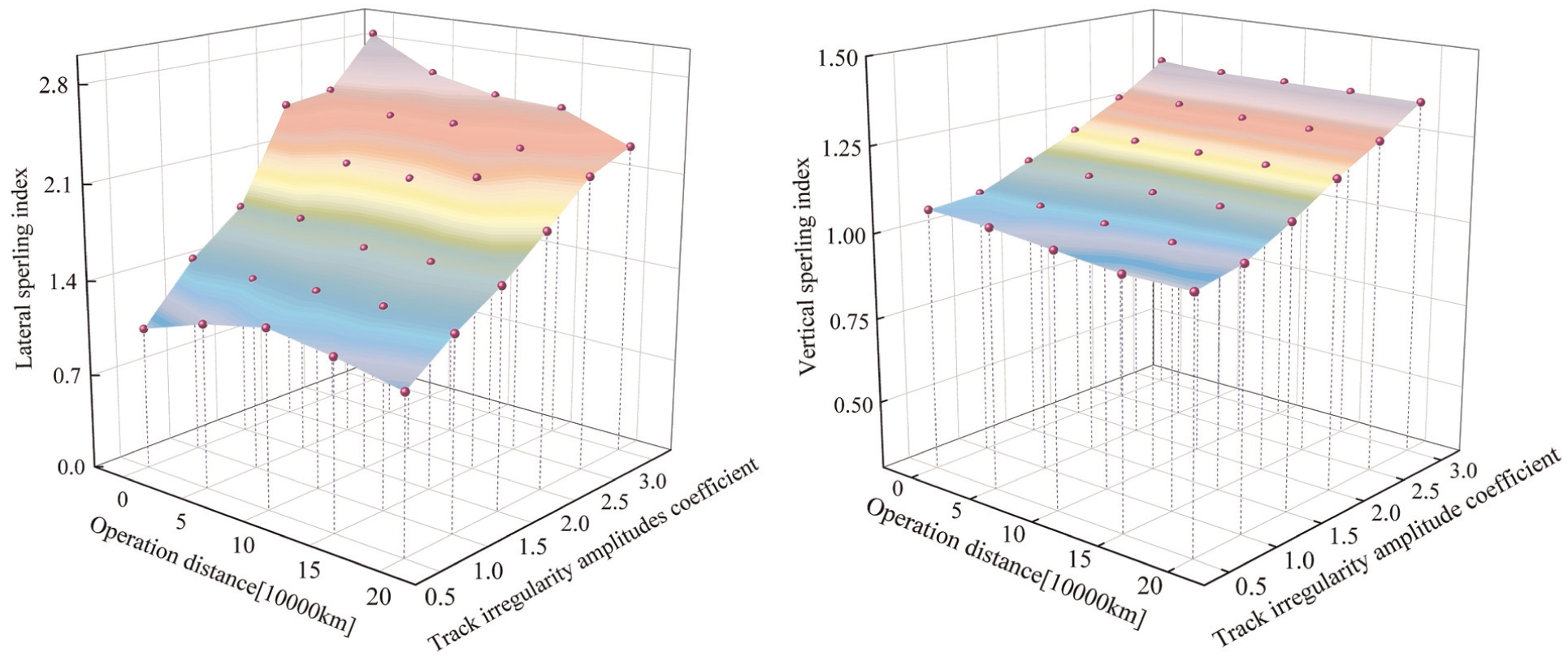
Sperling index at different operation distance and track irregularity amplitude coefficient (x-axis is the operation distance (×10,000 km), y-axis is velocity (km/h), z-axis is sperling index, the limited value is 3.00).

Safety analysis of vehicles negotiating curves

For derailment safety evaluation, the fundamental parameter is the derailment coefficient. According to Nadal,²⁷ the wheel flange begins to climb when the combined vertical component of the normal force and the friction creep force equals or exceeds the wheel load.

According to CEN 14363²⁸ and UIC 518,²⁹ the criterion $Y / Q (\leq 0.8)$ should be used:

{(\frac{Y}{Q})}_{lim} = 0.8 for R \geq 250 m

(1)

In addition, the wheel unloading rate is a critical factor in accurately assessing derailment safety. According to the established criteria,²⁶ the maximum wheel unloading rate must not exceed 0.8 to ensure safe operation.

Profiles covering 0–200,000 km were employed in the simulations, with vehicle profiles updated every 50,000 km. The results in Table 4 indicate that the critical amplitude coefficient decreases progressively with operation distance, reflecting a deterioration in running safety. At 0 km, the safety threshold is 3.5, as both derailment coefficient and wheel unloading rate exceed their limits when the amplitude coefficient reaches 3.6. With increasing mileage, the thresholds decline to 3.4, 3.2, and 3.1 at 50,000, 100,000, and 150,000 km, respectively. At 200,000 km, the derailment coefficient already exceeds the safe value when the amplitude coefficient is 3.1, although the wheel unloading rate remains within the limit, thereby setting the critical value at 3.0. Overall, the critical amplitude coefficient exhibits a nearly linear downward trend, with the most pronounced reduction of 5.9% observed between 50,000 and 100,000 km, and an average decrease of 0.025/10,000 km.

Table 4.

Derailment coefficient and wheel unloading rate under different operation distance.

Operation distance (10,000 km)	Amplitude coefficient	Derailment coefficient	Wheel unloading rate
0	3.6	−0.850	0.825
	3.5	−0.681	−0.727
5	3.5	−0.915	0.837
	3.4	−0.420	0.745
10	3.3	−1.970	−0.974
	3.2	−0.738	0.778
15	3.2	−2.238	0.812
	3.1	−0.305	0.790
20	3.1	−0.803	0.750
	3.0	−0.678	0.743

Due to centrifugal and inertial forces, high-speed trains can induce contact between the wheel flange and the rail, generating wheel–rail lateral forces. Figure 10 illustrates the influence of track irregularity amplitudes on the lateral forces of inner and outer wheels at different wear stages.

Figure 10.

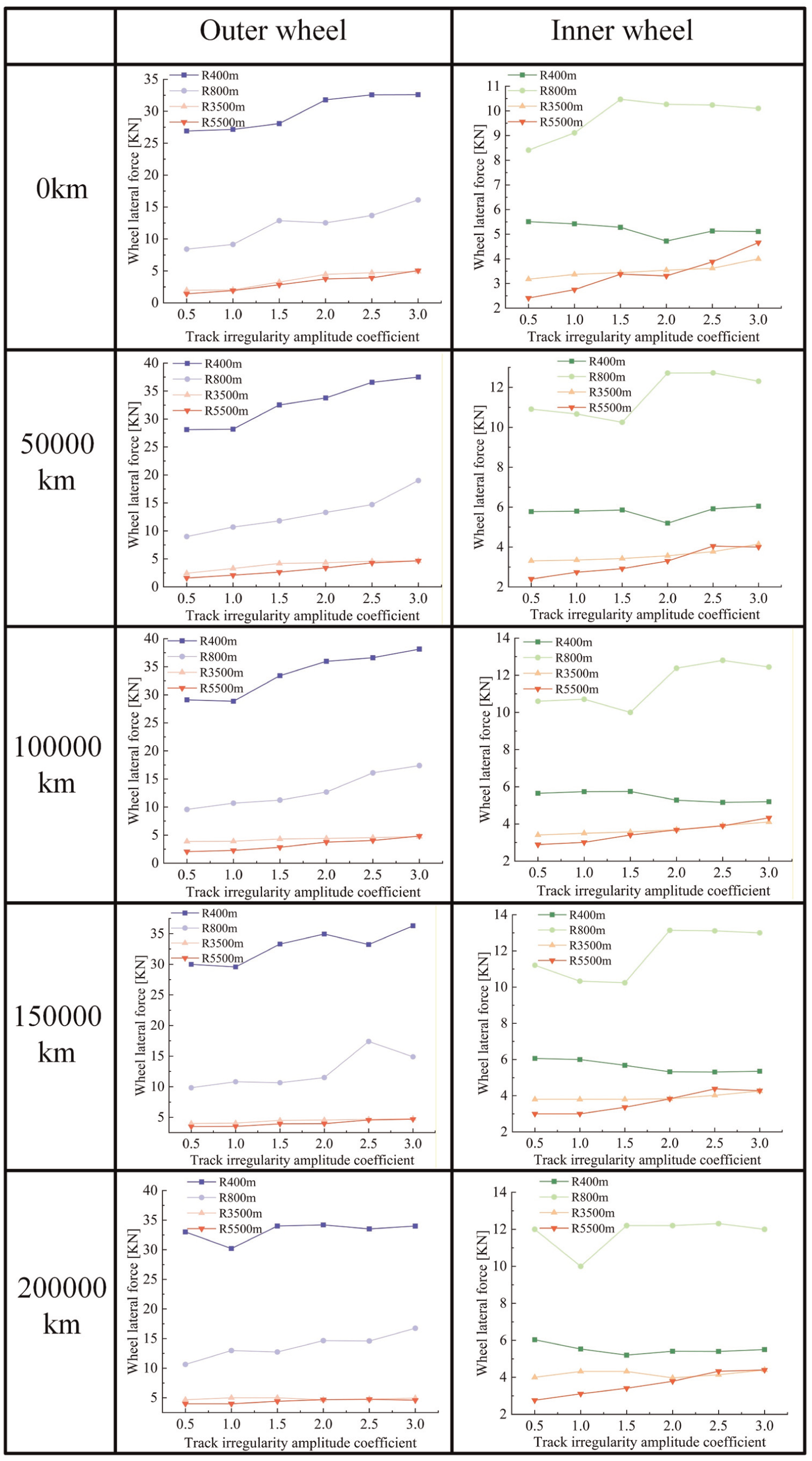
Wheel lateral force at different wear mileages and track irregularity amplitude coefficient.

Figure 11 illustrates the impact of curve radius and track irregularity amplitudes on wheel–rail lateral displacements at different wear mileages.

Figure 11.

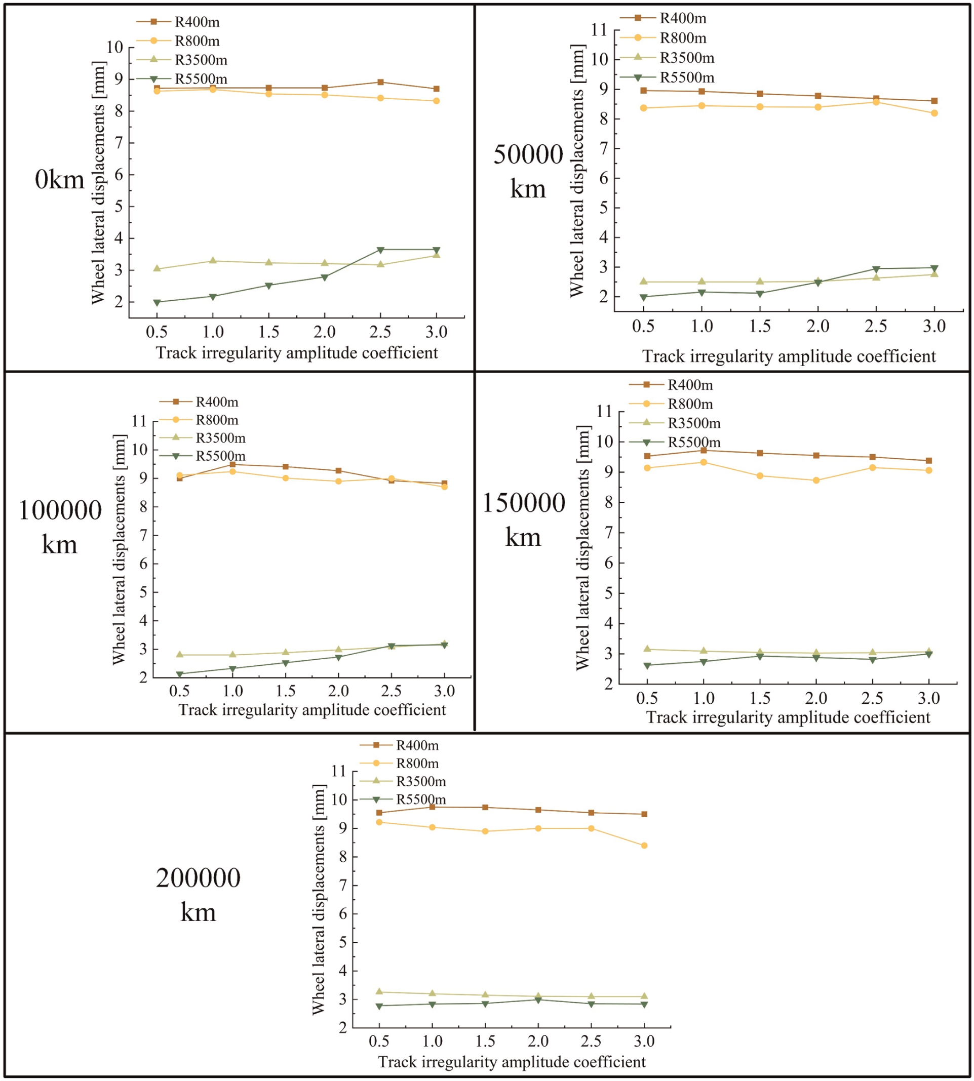
Wheelset lateral displacements at different wear mileages and track irregularity amplitude coefficient.

The lateral forces on the wheels have a significant impact on derailment, as the derailment coefficient is the ratio of lateral force to vertical force. Since the impact of irregularity amplitudes on the vertical direction is relatively small, it suggests that lateral forces play a more dominant role in derailment. The trend in the figure is clear: as track irregularity amplitudes increase, lateral forces tend to rise. It is evident that smaller curve radius result in higher lateral forces. The derailment coefficients for the vehicle negotiating curves with radius of 400, 800, 3500, and 5500 m are 1.30, 0.52, 0.20, and 0.32, respectively. It is important to note that the 400 m radius curve is a critical radius, where uneven loading between the inner and outer wheels occurs. The lateral force on the inner wheel is very small, while the lateral force on the outer wheel is significantly higher. As wear increases, the overall trend of the lateral force shows an increase. In the mid-wear stage, with a curve radius of 400 m and a track irregularity coefficient of 3.0, the lateral force on the outer wheel is 38.14 KN, intensifying the lateral impact between the wheel and rail. Reducing the speed to 84 km/h ensures that the derailment coefficient remains below 0.8.

As shown in the Figure 11, with both wear mileage and decreasing curve radius, the wheelset lateral displacement generally increases. By calculating the rate of change in lateral displacement for track irregularity coefficients of 0.5–1.0, 1.0–1.5, 1.5–2.0, 2.0–2.5, and 2.5–3.0, the maximum rates of change were found to be 8.9%, 8.6%, 7.9%, 14.6%, and 1%, respectively. The results indicate that the impact of track irregularity amplitudes on wheelset lateral displacement is relatively small. Notably, on the 5500 m radius curve, the changes are more pronounced compared to smaller radius curves, with the overall trend showing an increase in displacement as the amplitude coefficient increases, however, in the late wear stage, the changes become less significant.

The analysis under frozen conditions

The line in question is the Beijing–Shanghai line. According to surveys, the minimum temperature in Beijing can reach as low as −20 °C. Therefore, this study analyzes the operational performance with different worn wheel profiles and track irregularities under different frozen conditions at −20 °C. According to the Song and Luo,²⁰ the rotary arm positioning nodal points stiffness increases by 25%, the vertical stiffness of the air spring increases by 25%, the lateral stiffness increases by 30%, and the stiffness and damping of the damper increase by 30% and 20%, respectively. The CR400BF train was simulated on a curve with a radius of 10,000 m at a speed of 300 km/h. Since the temperatures in this scenario are not extreme and may not lead to snow accumulation on the tracks, this study does not account for variations in friction. According to Kloow,³⁰ the average density of ice ranges between 200 and 250 kg/m³. The bogie wheelbase of the train is 2.2 m, the lateral spacing between primary and secondary suspension elements is ∼2 m, the bogie height is about 1.36 m, and the envelope volume of the bogie is ∼5.984 m³. After subtracting the intrinsic volume, the effective volume is around 3.1 m³. Therefore, we assume a range of ice mass from 0 to 775 kg. The ice mass parameter ranging from 0 to 775 kg is discretized into 80 uniformly distributed working conditions and increases the moment of inertia for each mass condition in the bogie:

I_{ζ} = m_{i} \cdot L_{ζ}^{2} (i = 1, 2, 3 . . . . . ., 80)

(2)

where $ζ$ represents the frame coordinates (x, y, z), and $L_{ζ}$ is the moment of inertia matrix.

The impact of frozen conditions on the lateral acceleration of the bogie

Figure 12 shows the lateral acceleration RMS of the bogie under different frozen conditions. The acceleration limit for this model can be calculated as 5.65 m/s² based on the lateral acceleration RMS limit of the bogie specified in UIC 518.³¹

RM S_{lim} = \frac{12 - m_{z} / 5}{2}

(3)

where $m_{z}$ is the mass of the bogie.

Figure 12.

RMS of lateral bogie acceleration under different frozen conditions: (a) primary suspension frozen, (b) secondary suspension frozen, and (c) all suspension frozen.

As shown in Figure 12, the influence of wheel-profile wear on the RMS of lateral bogie acceleration is relatively small. Across the mileage range from 0 to 200,000 km, the RMS varies within ∼18%, and the minimum value appears at 50,000 km, where the RMS is about 15%–18% lower and more stable than the unworn condition. In contrast, the RMS shows a pronounced dependence on the amplitude of track irregularities. When the amplitude coefficient increases from 1.0 to 2.0, the RMS rises by more than 200%, and most values exceed the safety limit once the coefficient reaches 2.0, indicating that track irregularity is the dominant factor governing lateral dynamic response.

Suspension conditions introduce additional differences at a smaller magnitude. The RMS under secondary suspension frozen is generally 5%–10% higher than in the primary frozen condition, while the all frozen condition produces RMS levels comparable to or slightly lower than those under primary frozen. Overall, the quantitative results confirm that track irregularity amplitude and suspension state exert the primary control on lateral bogie acceleration, whereas the effect of wheel wear remains comparatively minor.

The impact of frozen conditions on Sperling index

As shown in Figure 13, wheel-profile wear has only a minor influence on the lateral Sperling index. Within the mileage range of 0 to 200,000 km, the median shows a slight decrease, dropping by ∼8%, and all cases remain firmly within the “excellent” comfort category. In contrast, the Sperling index is highly sensitive to the amplitude coefficient of track irregularities. When the amplitude coefficient increases from 1.0 to 1.5, the index rises by ∼10%–15%. From 1.0 to 2.0, the growth rate reaches 30%–40%, and from 1.0 to 2.5, the increase relative to the baseline is typically 50%–60%. Under primary suspension frozen, the index approaches the “acceptable” range once the coefficient reaches 2.0, whereas under secondary suspension frozen and the all frozen condition, similar comfort degradation occurs only at coefficients between 2.0 and 2.5, indicating stronger sensitivity.

Figure 13.

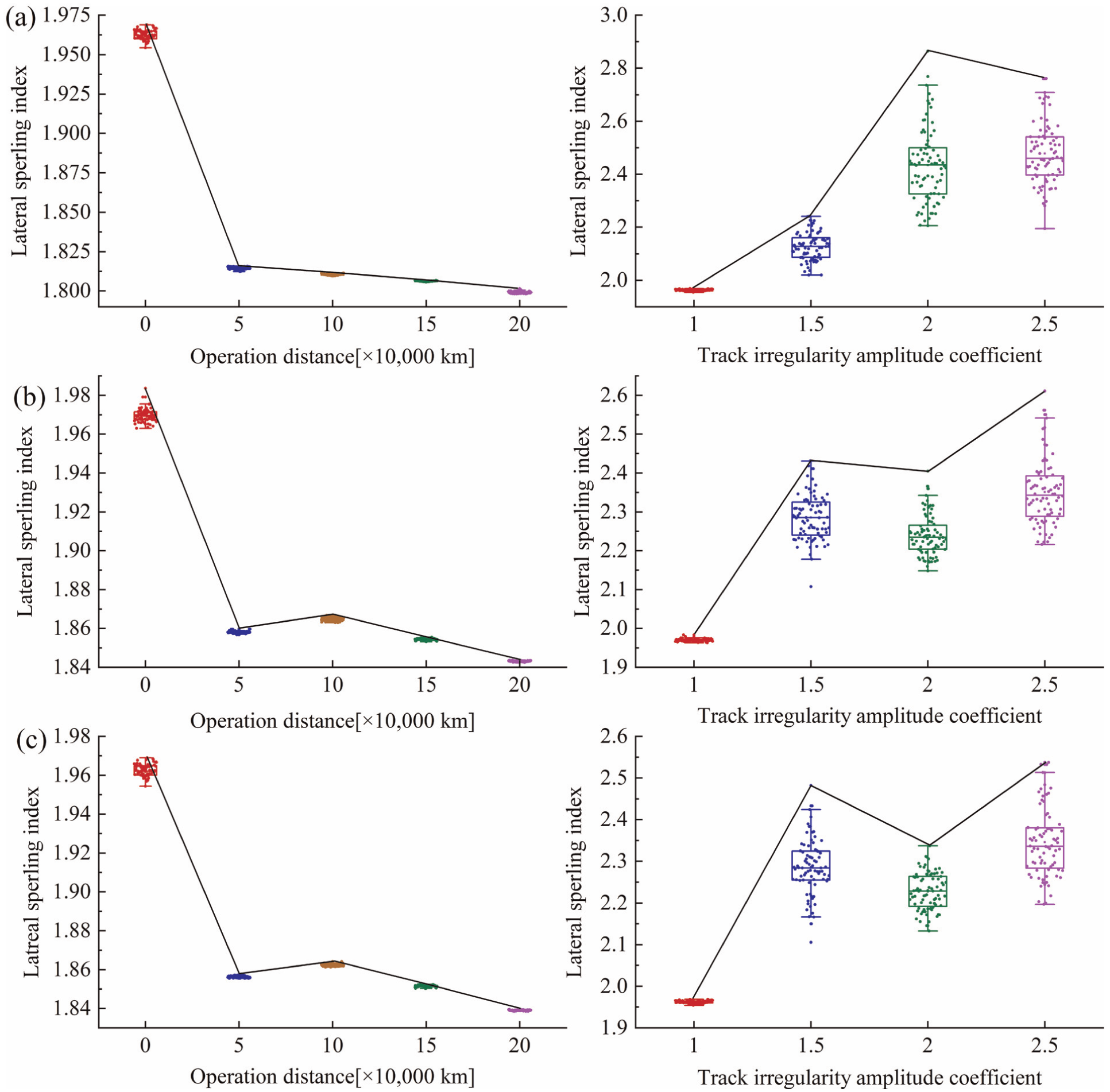
Lateral Sperling under different frozen conditions: (a) primary suspension frozen, (b) secondary suspension frozen, and (c) all suspension frozen.

The impact of frozen conditions on safety performance

As shown in Figure 14, the influence of wheel profile wear on the derailment coefficient is relatively limited. Quantitatively, under normal conditions, the derailment coefficient ranges between 0.31 and 0.46, remaining below the critical safety threshold of 0.8 across all operation distances. In contrast, track irregularity and suspension frozen have a stronger effect. Under primary suspension frozen conditions, the derailment coefficient exceeds the safety limit when the track irregularity amplitude coefficient reaches 2.0, with values ranging from 0.5 to 2.5 at this threshold and peaking at 3.2 for an amplitude coefficient of 2.5. For secondary suspension frozen and all suspension frozen cases, derailment occurs at a lower amplitude coefficient of 1.5, with maximum derailment coefficients reaching 2.7–3.0, demonstrating higher sensitivity to track irregularities.

Figure 14.

Derailment under different frozen conditions: (a) primary suspension frozen, (b) secondary suspension frozen, and (c) all suspension frozen.

The effect of ice mass is evident from the boxplots: larger ice accumulation increases the spread of the derailment coefficient. At higher amplitude coefficients, the range of derailment coefficients expands to 0.5–3.0, indicating a reduction in the safety margin. This quantitative evidence highlights that while wheel profile wear alone does not pose a significant derailment risk, the combined effects of suspension frozen, increased track irregularity, and ice accumulation can markedly increase derailment probability.

It can be observed from Figure 15 that under different wheel profiles, the wheel unloading rate exhibits a clear dependence on both wear mileage and track irregularity amplitude. Under the three conditions of primary suspension frozen, secondary suspension frozen, and all suspension frozen, the wheel unloading rate corresponding to the ice mass distribution shows a “first decrease then increase” trend with operating distance. When the operation distance is 0 km, the unloading rate drops from the initial 0.325–0.340 to a minimum value of about 0.300 (a decrease of 6%–12%) around 50,000 km. After the mileage exceeds 50,000 km, it gradually rises. By 200,000 km, the unloading rates of the three conditions reach 0.375, 0.370, and 0.380, respectively, which are 23%–27% higher than the minimum value.

Figure 15.

Wheel unloading rate under different frozen conditions: (a) primary suspension frozen, (b) secondary suspension frozen, and (c) all suspension frozen.

Meanwhile, the wheel unloading rate shows a strong positive correlation with the track irregularity amplitude coefficient. When the amplitude coefficient is 1, the unloading rate is 0.3. As the coefficient increases to 1.5, the unloading rate rises to 0.65. When the coefficient reaches 2.0, the unloading rate climbs to 0.82, which exceeds the safety threshold. Further increasing the coefficient to 2.5 results in an unloading rate of 0.85–0.90.

Conclusions

This study conducted tracking measurements of wheel wear on the Beijing–Shanghai high-speed railway and performed vehicle dynamic simulations under a coupled framework integrating wheel wear, track irregularities, and frozen conditions. A comprehensive analysis was carried out to evaluate the effects of wheel wear, track irregularity amplitudes, and ice mass under frozen conditions on vehicle dynamics. The main findings are as follows:

The study indicates that the vehicle speed is positively correlated with the lateral sperling index. Furthermore, the standard wheel is more sensitive to changes in track irregularity amplitudes compared to the worn wheel. When the track irregularity amplitude coefficient reaches 3.0, the standard wheel profile comfort index is worse than worn wheel, which significantly deteriorates the vehicle’s straight-line running performance.

Regarding curve passing performance, the study clearly shows that at a curve radius of 400 m, there is a significant uneven distribution of forces between the inner and outer wheels. In other words, there is a significant derailment risk on 400 m radius curves. Reducing the speed to 84 km/h ensures safety. According to safety simulations, the critical track irregularity amplitude coefficient at 200,000 km is 3.0. This suggests the potential to extend the intervals for both wheel reprofiling and rail grinding maintenance.

Under frozen conditions, the effect of the worn wheel profile is negligible. Meanwhile, simulations reveal that the 50,000 km wheel profile performs relatively well overall. However, the study shows that after the amplitude coefficient of track irregularities reaches 2.0, all indicators, except for the comfort index, exceed the critical threshold. The more severe the suspension freezing, the more sensitive the ice mass is to the derailment coefficient. When the track irregularity amplitude coefficient reaches 1.5, more indicators exceed the critical value.

Considering all factors, the wheel profile at around 50,000 km can be used as the optimized profile. Under non-frozen conditions, the rail can be ground when the track irregularities’ amplitude reaches −6 to 6 mm, this approach ensures both ride comfort and vehicle operational safety. The specific method should be determined by engineers based on the actual conditions. For a 400 m curve radius, the speed must be reduced to 84 km/h to ensure safety. The proposed dynamic research methodology can be widely applied to other vehicles. The impact of track excitation is not limited to amplitude, wavelength is also highly important. In our subsequent work, based on the findings of this paper, we will analyze the effects of complex track excitations that consider both wavelength and amplitude.

Footnotes

Handling Editor: Chenhui Liang

ORCID iD

Xikang Hu

Funding

The authors disclosed receipt of the following financial support for the research, authorship, and/or publication of this article: the China Academy of Railway Sciences Group Co., Ltd. Program (2022YJ303) and the Open Project Fund of National International Science and Technology Cooperation Base on Railway Vehicle Operation Engineering of Beijing Jiaotong University (BMRV21KF01).

Declaration of conflicting interests

The authors declared the following potential conflicts of interest with respect to the research, authorship, and/or publication of this article.

References

Barke

Chiu

WK.

A review of the effects of out-of-round wheels on track and vehicle components. Proc Inst Mech Eng F J Rail Rapid Transit 2005; 219: 151–175.

Peng

Simon

Philip

, et al. General conditions for railway wheel polygonal wear to evolve. Veh Syst Dyn 2021; 59: 568–587.

Pradhan

Samantaray

Bhattacharyya

Prediction of railway wheel wear and its influence on the vehicle dynamics in a specific operating sector of Indian railways network. Wear 2018; 406–407: 92–104.

Hou

Chen

Cheng

Study on the evolution of wheel wear and its impact on vehicle dynamics of high-speed trains. Coatings 2022; 12: 1333.

Zhu

Yang

, et al. Effects of different wheel wear positions on dynamic performance of metro vehicles. Ind Lubr Tribol 2023; 75: 305–314.

Zhu

, et al. Influence of wheel profile wear coupled with wheel diameter difference on the dynamic performance of subway vehicles. Shock Vib 2021; 2021(8): 1–15.

Seo

Hur

Kwon

SJ.

Effect of mechanical properties of rail and wheel on wear and rolling contact fatigue. Metals 2022; 12: 630.

Yang

Tao

, et al. On the formation mechanism of high-order polygonal wear of metro train wheels: experiment and simulation. Eng Fail Anal 2021; 127: 105512.

Polach

Nicklisch

Wheel/rail contact geometry parameters in regard to vehicle behaviour and their alteration with wear. Wear 2016; 366–367: 200–208.

10.

Enblom

Deterioration mechanisms in the wheel–rail interface with focus on wear prediction: a literature review. Veh Syst Dyn 2009; 47: 661–700.

11.

Zhu

Yang

, et al. Simulation and measurement study of metro wheel wear based on the Archard model. Ind Lubr Tribol 2019; 71: 284–294.

12.

Choi

IIY

J-H

Lee

, et al. The influence of track irregularities on the running behavior of high-speed trains. Proc Inst Mech Eng F J Rail Rapid Transit 2012; 227: 94–102.

13.

Liu

Thompson

Griffin

, et al. Effect of train speed and track geometry on the ride comfort in high-speed railways based on ISO 2631-1. Proc Inst Mech Eng F J Rail Rapid Transit 2019; 234: 765–778.

14.

Xin

Wang

Ding

Effect of long-wavelength track irregularities on vehicle dynamic responses. Shock and vibration 2019; 2019(3): 1–11.

15.

Chang

Cai

Wang

, et al. The influence of track irregularity in front of the turnout on the dynamic performance of vehicles. Appl Sci 2022; 12: 9.

16.

Bosso

Bracciali

Megna

, et al. Effects of geometric track irregularities on vehicle dynamic behaviour when running through a turnout. Veh Syst Dyn 2023; 61: 782–798.

17.

Hong

Zhang

, et al. Numerical simulations of snow accumulation in the bogie region of a train considering snow particle rotation. Fluid Dyn Mater Process 2024; 20: 2337–2352.

18.

Teng

Luo

Shi

, et al. Dynamics behaviour of high-speed train at the low temperature of −40 °C. J Mech Eng 2019; 55: 148–153.

19.

Gao

Zhang

Wang

Numerical and experimental investigation on snow accumulation on bogies of high-speed trains. J Central South Univ 2020; 27: 1039–1053.

20.

Song

Luo

. Study on the impact of suspension parameter changes under low temperature conditions on dynamic performance. In: Proceedings of the 8th China intelligent transportation annual conference, Anhui, China, 26 September 2013, paper no. U270.33, pp.309–314. China Intelligent Transportation Association.

21.

Luo

Teng

, et al. Dynamics simulation of a high-speed railway car operating in low-temperature environments with stochastic parameters. Veh Syst Dyn 2020; 58: 1914–1934.

22.

Sun

LX.

Rolling contact fatigue analysis and mitigation strategies based on wheel wear after 200,000 km. Ind Lubr Tribol 2025; 77(10): 1661–1673.

23.

Hertz

On the contact of elastic solids. Crelle’s J 1881; 146: 22–34.

24.

Kalker

JJ.

A fast algorithm for the simplified theory of rolling contact. Veh Syst Dyn 1982; 11: 1–13.

25.

Xiang

Cheng

, et al. Statistical analysis on ballastless track spectrum of high-speed railway. J Railw Sci Eng 2016; 13: 1659–1666.

26.

Ren

ZS.

Railway vehicle system dynamics. China Railway Publishing House, 2019.

27.

Nadal

. Locomotives à vapeur, collection encyclopédie scientifique. Bibliothèque de Mécanique Appliquée et Génie 1908; 186(1): 56–67.

28.

CEN 14363: 2007. Railway applications – Testing for the accptance of running characteristics of railway vehicles – Testing of running behaviour and stationary tests.

29.

UIC 518: 2005. Testing and approval of railway vehicles from the point of view of their dynamic behaviour – safety – track fatigue – ride quality.

30.

Kloow

. High-speed train operation in winter climate. Foreign Rolling Stock 2015; 52(01): 1–10.

31.

UIC 518: 2009. Testing and approval of railway vehicles from the point of view of their dynamic behavior – safety – track fatigue – ride quality.

The impact of wheel wear and track irregularity amplitudes on the operation of high-speed trains

Abstract

Keywords

Introduction

Wheel–rail coupling dynamics model

Modeling and analysis

Model of wheel–rail contact interactions

Selection and scaling of track irregularities

Wheel wear analysis within one reprofiling cycle

Measured wheel wear evolution

Analysis of measured wear depth

Impact of wheel wear and track irregularity on dynamics

Ride comfort analysis

Safety analysis of vehicles negotiating curves

The analysis under frozen conditions

The impact of frozen conditions on the lateral acceleration of the bogie

The impact of frozen conditions on Sperling index

The impact of frozen conditions on safety performance

Conclusions

Footnotes

ORCID iD

Funding

Declaration of conflicting interests

References