Sage Journals: Discover world-class research

Abstract

This paper studies the Job Shop Scheduling Problem (JSSP) with Unit Processing Times evolving in an uncertain environment. Our aim is to determine a set of solutions instead of a unique solution in order to manage unanticipated events. To achieve this, an approach integrating two techniques is presented to achieve sequential flexibility. In the first time, the decomposition of the initial problem into sub-problems is exploited for producing a dominant schedule. Then, based on the Group Sequence (GS) method, a set of schedules is constructed, allowing for sequential flexibility with an evaluation of performance. The present work also develops a new lower bound for the GS and compares it with an existing lower bound from the literature. Using benchmark data sets, computational studies demonstrate that the suggested lower bound significantly outperforms the established lower bound found in the literature. In addition, our approach succeeded in finding a set of solutions for all tested benchmarks within a reasonable amount of CPU time. Moreover, two interesting flexibility indicators are presented to evaluate the efficacy of our approach.

Keywords

production scheduling uncertain environment group sequence sequential flexibility unit processing times lower bound

Introduction

In the current era of digital manufacturing technologies, combined with uncertain manufacturing environments, production scheduling represents a strategic problem for companies. Scheduling involves allocating a restricted number of machines to a set of jobs within a specific time horizon while satisfying a set of constraints and optimizing one or more objective functions.¹ To solve this problem, many research work has focused mainly on proposing exact and approximate methods to find optimal or near-optimal solutions. These methods adopted deterministic assumptions and considered static environments, where all parameters were known in advance and remained constant over time. However, not all information is known with certainty in real-world production systems, and the environment is naturally dynamic where many disruptions might arise, such as the arrival of new jobs,² machine breakdowns,^3–5 processing time variations,⁶ etc. In recent years, scheduling under uncertainty has received a lot of interest within the research community. Different methods have been proposed in the literature to deal with such uncertainty, often referred to as robust approaches, with the aim of generating schedules that remain valid and effective even when disruptions occur. These methods seek to respond to practical challenges where flexibility and reactivity are essential to managing uncertainties.^7,8 In this context, there are generally three categories of approaches: proactive (offline scheduling), reactive (real-time scheduling), and proactive-reactive.

Scheduling problem with unit processing times is a special case of the general scheduling problem. When assuming that all jobs have the same processing time, it is to simplify the problem and provide a way of managing mass production.⁹

JSSP with unit processing times is the most common configuration in industries where operations are standardized and have similar durations. Typical examples include electronic component testing, printed circuit board assembly, and surface treatment workshops, where each job goes through a series of short and similar operations on different machines. In such environments, uncertainty can arise from unexpected machine stoppages, material delays, or priority changes. Therefore, the main challenge is to organize and assign tasks efficiently under uncertainty rather than to handle variations in processing times. Despite its simplified processing assumptions, the JSSP with unit processing times remains an NP-hard combinatorial optimization problem, making its resolution computationally challenging even for medium-sized instances.¹⁰ Introducing uncertainty into this already complex problem further increases its difficulty, as it requires developing more robust and adaptive scheduling strategies.

The primary aim of our research is to address the JSSP with equal processing times, by drawing inspiration from the most effective proactive–reactive strategies highlighted in the literature. To the best of our knowledge, no prior study has tackled the JSSP with equal processing times under uncertainty, despite its clear practical relevance. In contrast, this work introduces a novel robust approach that takes into account the uncertain environment of real life. It aims to deliver robust solutions that, although sometimes of lower quality, are often preferred by decision-makers for their greater resilience compared to vulnerable optimal ones. The main contributions of this work are:

The generation of a set of feasible schedules instead of a single one, enabling both proactive and reactive decision-making.

A solution set defined via the GS method, characterized by best and worst-case execution times for each operation.

The identification of a new lower bound, based on the best-case performance, which outperforms several benchmarks from existing studies.

The introduction of two flexibility indicators to evaluate the robustness and adaptability of the proposed solutions.

The remainder of this paper is structured as follows: the next section presents the literature review on scheduling under uncertainty and scheduling problems with unit processing times. The description of the issue and its representation as a disjunctive graph are given in Section “Problem statement.” In Section “Problem decomposition and dominant sequences,” a decomposition of the global problem into several local scheduling that provide sequential flexibility is detailed. In Section “Group sequence based approach,” the construction of a solution set and the determination of a lower bound are presented using the GS method. Section “Computational experiments” presents and discusses the computational results. Finally, Section “Conclusion” summarizes the contribution with future research directions.

Literature review

This section reviews related research. The first subsection presents main approaches for scheduling under uncertainty, while the second examines studies addressing scheduling problems with unit processing times.

Scheduling under uncertainty

Scheduling under uncertainty has been widely studied to address the variability that affects real production systems. Depending on the timing and availability of information, three main approaches are generally distinguished: offline (proactive), online (reactive), and hybrid (proactive–reactive) methods.

Reactive scheduling occurs at the time of executing a predictive schedule by adjusting it so as to take into account the current state of the system. In this context, Ghaleb et al.¹¹ have developed real-time scheduling models to resolve a flexible job shop scheduling problem (FJSSP) subjected to two types of disruptions: machine breakdowns and the arrival of new jobs. In line with this, Zhou et al.¹² studied a scheduling problem in cloud manufacturing services and proposed a purely reactive approach based on an event-triggered strategy that took into account the arrival of new jobs. Considering both the setup time and the random arrival of jobs in the dynamic job shop scheduling problem (DJSSP), the authors in Zhang et al.¹³ have proposed an improved gene programming algorithm to construct scheduling rules. Later, an effective decision-making algorithm is proposed in Zhang and Buchmeister¹⁴ to solve the DJSSP optimization problem. The authors proposed an improved multiphase particle swarm optimization and showed the high level of robustness of their approach.

In contrast to the reactive approach, the proactive approach takes into account the uncertainty when establishing the predictive schedule. The schedule is then more robust as it remains valid even when disturbances occur. Often flexibility is used and is defined as the property of having the potential to satisfy performance requirements.¹⁵ These techniques have also attracted the attention of many researchers. Wang et al.¹⁶ proposed two robust scheduling formulations for JSSP in a realistic production system with uncertainty of processing time, based on a set of bad scenarios. Another study was conducted by Wang et al.¹⁷ to resolve a proactive scheduling problem in a steel production system, considering both stochastic machine breakdown and processing time to achieve a robust predictive schedule. Parallely, Xiao et al.¹⁸ have discussed robust JSSP under processing time variations. Robustness was measured by the deviation between the realized makespan and the predictive makespan. A surrogate model was offered to optimize both scheduling performance and robustness. In Grumbach et al.,¹⁹ the authors have considered a dynamic production system and integrated regression models into a metaheuristic model to predict makespan robustness and to deal with uncertain processing times.

In reality, proactive scheduling and reactive scheduling are closely intertwined. In fact, it is unlikely that all unforeseen events will be predicted in advance. It is worth mentioning the work of Davari and Demeulemeester²⁰ where they have considered the project scheduling problem with stochastic processing time and formulated the problem as an integrated proactive and reactive scheduling problem. They showed that their model outperformed the traditional models. In addition, within the framework of these types of approach, one of the most successful methods used in the literature is the Groups of Permutable Operations method (GoPO),^21,22 commonly called the “Group Sequence” (GS) method. It assigns an ordered partition of operations to each machine, that is, a group sequence.^23–26 The principle of this approach consists of building, in a predictive manner, a set of flexible solutions without enumerating them. This representation allows us to choose the most adapted solution to react to unexpected events during the reactive phase. An important characteristic of this approach is that it can ensure, admittedly, the existence of a solution computable in polynomial time²⁴ with a quality, in the worst case, lower than the non-robust optimal solution, and can thus be used during the reactive phase of the GS schedule. Still in the same context, other approaches that exhibit sequential flexibility were proposed, which is less restrictive than the GS method. These approaches are based on a dominance theorem that generates a dominant partial order between tasks.²⁷ In Briand et al.,²⁸ the authors proposed a robust approach for the single machine scheduling problem that characterizes a large set of optimal schedules regarding the lateness criterion.

A review of the literature reveals that robust approaches are becoming more and more popular because in real-world environments, unexpected events and data uncertainty are challenging the planned plans, making them ineffective. Reactive approaches do not create a plan in advance but react to events when they arise. They calculate in real-time the best possible scheduling, taking into account the type of uncertainties. The disadvantage is that the solution is often unstable, and frequent changes may disrupt the remaining steps of the process. Proactive approaches aim to anticipate problems before they occur. They create a schedule in advance and at the beginning, taking into account prior knowledge of probable uncertainties to absorb potential disruptions. The schedule in this case does not require frequent adjustments, but its efficiency may be reduced since it is unrealistic to proactively take into account all the unexpected events that may arise. The proactive-reactive approach is a combination of two previous ones, and it is the most common approach used in complex and uncertain production environments. They are not only interested in providing a unique schedule accounting for the most common and probable disruptions, but also in determining a flexible set of baseline schedules, thereby offering more choices during the reactive phase.

A key strength of our approach lies in the sequential flexibility it offers. Rather than producing a single static schedule, it generates a set of feasible alternatives offline, allowing real-time adaptation to disruptions by switching between solutions without significant performance loss. This approach combines two complementary techniques. First, the problem is decomposed into several single-machine sub-problems (as in Erschler and Roubellat²⁹) to establish a partial order between operations and handle sequential flexibility. Then, drawing from the GS method,²² groups of fully permutable operations are constructed to generate a set of robust schedules with measurable performance. This framework ensures proactive flexibility during the planning phase while enabling reactive adaptation during execution.

Scheduling problem with unit processing times

The scheduling problem with unit processing times has attracted the interest of many researchers in the literature. In the field of single-machine scheduling with unit processing times, many recent studies have made important contributions, considering total completion times and the number of late jobs as criteria to minimize.^30,31 Chen et al.³² have applied the concept of two agents to a one-machine scheduling problem where the jobs of each agent have their own equal processing times. Their analysis reveals the binary NP-hardness of the problem depending on the criterion chosen for each agent. The research in Shen et al.³³ investigated the problem of scheduling jobs with equal processing times on uniform machines to optimize the total weighted completion time and the total tardiness simultaneously. Considering a parallel problem with identical execution times of jobs, the authors of Kravchenko and Werner³⁴ addressed a survey. By assigning jobs to machines sequentially, the open-shop scheduling problem with unit processing times was studied by van Bevern and Pyatkin.³⁵ They showed that the problem can be solved effectively in polynomial time. In the context of parallel machine scheduling with unit processing times, only a few studies have addressed this problem. One study considers a parallel machine scheduling problem and proposes both an optimal offline algorithm and an online algorithm with a competitive ratio matching the lower bound.³⁶ In the same line of research, another study develops an online algorithm for identical parallel machines with the makespan criterion, where jobs arrive sequentially and must be assigned immediately without knowledge knowing the release times of future tasks.³⁷ In Sotskov and Mihova,³⁸ the authors addressed multiprocessor unit scheduling tasks and solved them as an optimal mixed graph coloring problem with makespan and Lateness criteria.

Despite its practical importance, the JSSP with unit processing times has received limited attention in the literature, primarily due to its high computational complexity, even though it remains theoretically challenging and industrially relevant. In this context, the problem of minimizing the completion time has been shown to be equivalent to an optimal mixed graph coloring,³⁹ for which branch-and-bound algorithms have been developed to obtain optimal solutions. In another study, for solving large problem instances, a metaheuristic was developed in Kouider et al.¹⁰ A review of recent research on mixed graph coloring is provided in Sotskov.⁴⁰ However, the JSSP with unit processing and two objective functions, the makespan and the total completion time, was studied in Kouider and Haddadene.⁴¹ The authors modeled the problem as a bi-objective mixed graph coloring and proposed a resolution approach based on the branch-and-bound method. Beyond parallel machine environments, another line of research has examined multiprocessor scheduling problems.

The main studies addressing scheduling problems with unit processing times are summarized in Table 1.

Table 1.

Summary of studies on scheduling problems with unit processing times.

Problem type	Method	Objective	Nature	Reference
Single-machine, two-agent	Exact methods (polynomial and pseudo-polynomial algorithms)	Minimizing weighted sum of completion times and weighted number of tardy jobs	Deterministic	³⁰
NP-hard-single-machine	Polynomial-time exact algorithms	Minimizing maximum lateness L_max	Deterministic	³¹
Two-agent single-machine	Pareto optimization	Minimizing total tardiness, late work, weighted completion time	Deterministic	³²
Uniform machines	Exact polynomial algorithms	Total weighted completion time or total tardiness	Deterministic	³³
Parallel machine	Survey of exact and heuristic deterministic methods	Various	Deterministic	³⁴
Routing open shop	Theoretical analysis + integer linear programming + fixed-parameter algorithms	Minimizing makespan (C_max)	Deterministic	³⁵
Parallel machines	Offline exact algorithm (proactive) + online competitive algorithm (reactive)	Minimizing C_max	Under uncertainty	³⁶
Parallel machines	Optimal online algorithms (reactive)	Minimize C_max	Under Uncertainty	³⁷
Multiprocessor scheduling	Mixed graph coloring	Minimize C_max and L_max	Deterministic	³⁸
JSSP	Exact (bounds, MILP) + Heuristic (Tabu Search)	Minimizing C_max	Deterministic	¹⁰
JSSP and related scheduling problems	Mixed graph coloring	Minimizing C_max	Deterministic	⁴⁰
JSSP	Bi-objective Branch-and-Bound and ϵ - bi-objective mixed graph coloring;	Makespan and total completion time	Deterministic	⁴¹
JSSP	Decomposition into sub-problems combined with the (GS) method (proactive-reactive)	Minimize makespan and generate a set of flexible schedules	Under uncertainty	This work

Most of the previous works, summarized in Table 1, assume deterministic environments where all information is known in advance. Among them, only two works consider uncertainty: the first proposes both an offline exact algorithm and an online competitive algorithm for parallel machines,³⁶ while the second develops optimal online algorithms for the same context.³⁷ However, for scheduling problems with unit processing times, no study has simultaneously integrated a proactive–reactive method. Moreover, within the JSSP with unit processing times framework, no work has been conducted under uncertainty, nor has any approach aimed to generate a flexible set of solutions capable of adapting to unexpected disturbances, which remains an open and unexplored area.

Problem statement

The job shop scheduling problem with unit processing times $J_{n} | p_{i} = p | C_{\max}$ consists of scheduling a set of n jobs, represented by $J = {J_{1}, J_{2}, \dots, J_{n}}$ , that must be performed on a set of M machines = ${M_{1}, M_{2}, \dots, M_{m}}$ . A job $J_{j} (j = 1 . . . n)$ consists of multiple operations $O_{jk} (k = 1 . . . n_{j})$ that must be executed sequentially on the set of machines m according to the technological constraint. Any operation O_jk is executed on a single machine M_k, and is characterized by a release date r_jk, a due date d_jk, and a processing time $p_{jk} = p$ . We notice that in this study $n_{j} = m (j = 1 . . . n)$ . Every machine can handle only one non-preemptive operation at a time. The goal is to find a set of robust schedules while considering the maximum completion time C_max(makespan).

In this work, the scheduling problem with equal processing time (where $p_{jk} = p$ ) is equivalent to scheduling with unit processing time (where p_jk=1). This is due to the fact that the makespan scales linearly with p, and the constraints are only linked to the order of operations. We highlight that the experimental part will be done with p_jk=1 and the results remain valid for any constant p while the objective function $C_{\max} (p_{jk} \neq 1)$ is equal to $p \times C_{\max} (p_{jk} = 1)$ .

It is important to note that this problem is classified as NP-hardfor n > 2.^10,42

To simplify our notation, we use an equivalent representation of the problem throughout the rest of this paper. Given a job J_j, the index jk of operation O_jk is replaced by a single index O_i with $i = 1 . . . n \times m$ ; the total operations of all jobs being n × m. Hence, for each job instance j with n_j tasks, it assumes that all the job’s tasks pass through all the machines (i.e. square instance with task n_j=m).

The most popular model in the literature to represent a scheduling problem is the disjunctive graph $G (V, A, E)$ .⁴³ In this graphical representation, each vertex $v \in V$ symbolizes an operation of a job. Any two consecutive operations of the same job are connected by conjunctive arcs of A ensuring the precedence constraint. Any two operations sharing the same resource are linked by a disjunctive arc of E. For every pair of vertices connected by a conjunction arc, we assign a number that represents the processing time of the operation corresponding to the initial vertex. Furthermore, we add 0 and f two dummy operations having zero processing time, to the graph that correspond to the beginning and end of the set of operations. Any feasible solution is determined by orienting each disjunctive arc in a unique direction so that the resulting graph is circuit-free. The critical path corresponding to the longest path from the source vertex 0 to f corresponds to the makespan.

In more detail, each arc has a length, with an initial extremity representing the release date r_i and a final extremity representing the due date d_i.⁴³ Notice that r_i and d_i values are calculated using the Ford-Bellman algorithm⁴⁴ according to the following formulas:

r_{i} = L (0, i)

(1)

d_{i} = L (0, f) - L (i, f) + p_{i}

(2)

where $L (i, j)$ represents the longest path between task i and task j on the conjunctive graph and $L (0, f)$ represents the length of the longest path between 0 and f.

Definition 1. Given a $J_{n} | p_{i} = p | C_{\max}$ problem with m machines, n×m tasks, and its corresponding disjunctive graph, an initial structure of the problem (IS) is defined by r_i and d_i computed by equations (1) and (2) respectively, considering only conjunctive arcs.

Proposition 1. Given a $J_{n} | p_{i} = p | C_{\max}$ problem and its initial structure (IS) then, for each couple of tasks $(i, i + 1)$ such as $i ≺ i + 1$ , $r_{i + 1} = r_{i} + p$ , and $d_{i} = r_{i + 1}$ .

Proof. First, according to Definition 1 of an (IS), disjunctive arcs are not considered. Consequently, the starting time of any task $i + 1$ of a job depends only on its predecessor i. So, $r_{i + 1} = L (0, i + 1) = \sum_{j = 1}^{i + 1} p_{j} = (i + 1) p$ as p_i=p, that is, $r_{i + 1} = (i + 1) p = i . p + p = r_{i} + p$ . On the other hand, ${L (0, f) = m a x_{j = 1 \dots n} (\sum_{i = 1}^{n_{j}} p_{i}) = m a x_{j = 1 \dots n} (n_{j} . p) = m . p)$ as p_i=p and n_j=m. Similarly, $L (i, f) = (m - i) . p$ . Hence $d_{i} = L (0, f) - L (i, f) + p = sp$ ; $m . p - (m - i) . p + p) = (i + 1) p$ , that is, $d_{i} = ip + p = r_{i} + p = r_{i + 1}$ .

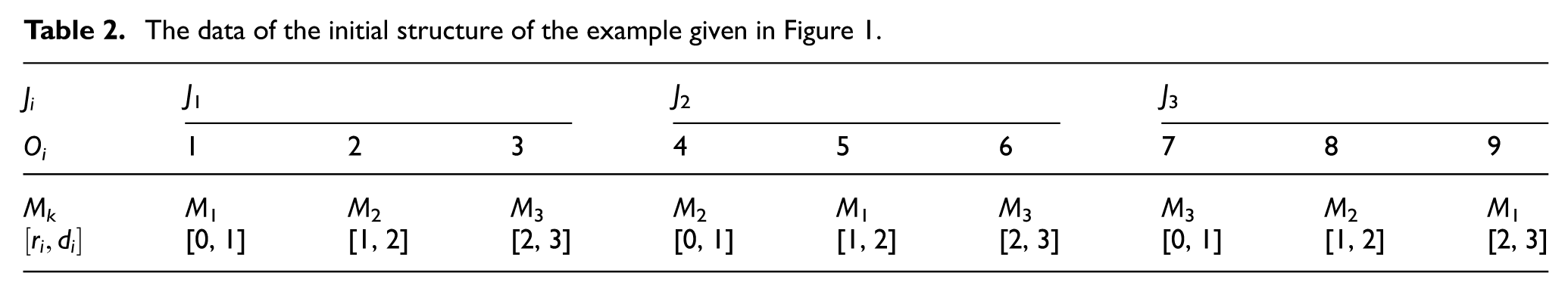
To illustrate this problem, an example of JSSP involving three jobs and three machines with unit processing times $J_{3} | p_{i} = 1 | C_{\max}$ is used. Each job consists of three operations, which must be executed sequentially on the three machines according to the job’s processing order. The disjunctive graph is shown in Figure 1.

Figure 1.

The disjunctive graph of an example problem with three jobs and three machines $J_{3} | p_{i} = 1 | C_{\max}$ .

In the initial structure of the JSSP $J_{3} | p_{i} = 1 | C_{\max}$ , the disjunctive arcs are not considered. The application of Proposition 1 returns the results in Table 2.

Table 2.

The data of the initial structure of the example given in Figure 1.

$J_{i}$	J ₁			J ₂			J ₃
O _i	1	2	3	4	5	6	7	8	9
M _k	M ₁	M ₂	M ₃	M ₂	M ₁	M ₃	M ₃	M ₂	M ₁
$[r_{i}, d_{i}]$	[0, 1]	[1, 2]	[2, 3]	[0, 1]	[1, 2]	[2, 3]	[0, 1]	[1, 2]	[2, 3]

Problem decomposition and dominant sequences

In this section, considering the JSSP with equal processing times, we propose a new scheduling approach with uncertainties. It is part of a robust approach and allows one to anticipate and react in real time to disturbances. The approach is based on the decomposition of the global problem into several local schedulings that provide sequential flexibility by exploiting a known dominance condition.

Local scheduling

Since the problem $J_{n} | p_{i} = p | C_{\max}$ is NP-hard, it is possible to decompose the initial problem into m interdependent single-machine sub-problems where each operation i of the job j is characterized by an execution window $[r_{i}, d_{i}]$ .²⁹ The sub-problems are interdependent because any sequence of operations determined on a given machine must be coherent (in terms of routing of jobs or workflow) with the sequences of operations of the other machines. The global JSSP, where the objective is to minimize the makespan is equivalent to a set of local schedules whose objective is to minimize the maximum lateness (problem noted ( $1 | r_{i} | L_{\max}$ ).⁴⁵

In this paper, the basic idea of the proposed robust approach is to define for each machine a set of dominant solutions instead of one optimal solution that can be used in real time during execution. Sequential flexibility is then used, and it is based on partial orders between tasks belonging to the same machine. The partial order is associated with the interval structure defined by the relative order of the release r_i and due dates d_i of tasks.²⁷

Interval structure and dominance principle

An interval structure is a model for representing temporal information. It describes a hierarchical representation of relationships between temporal intervals using constraints. An interval structure can be defined by a set of intervals I and a set of constraints C over I × I. Each interval x is defined by a lower bound (release date r_x) and an upper bound (deadline d_x). Any constraint between two intervals can be expressed using the relations of the algebra proposed in Allen.⁴⁶ Table 3 depicts the basic relations that can be defined between two intervals A and B using Allen’s algebra.

Table 3.

Allen’s algebra.

By considering Allen’s algebra, two particular types of intervals can be distinguished: top and base.⁴⁴

Definition 2. An interval s is a top of an interval structure $〈 I, C 〉$ if there is no interval $i \in I$ such that $during (i, s)$ , this means $r_{i} < r_{s} \land d_{i} > d_{s}$ , $\forall i \in I$ .

Definition 3. An interval b is a base of an interval structure $〈 I, C 〉$ if there is no interval $i \in I$ such that $during (b, i)$ , this means $r_{i} > r_{b} \land d_{i} < d_{b}$ , $\forall i \in I$ .

The notion of top has allowed to define the notion of s-pyramid that contains the top s and possibly other intervals.

Definition 4. A s-pyramid P_s associated with the top s is the subset of intervals $i \in I$ such that $during (i, s)$ holds. $P_{s} = {i \in I | r_{i} < r_{s} \land d_{i} > d_{s}} \cup {s}$

These concepts were used by Erschler et al.²⁷ for the one-machine scheduling problem with execution windows. They highlight a new dominance condition, relative either to the admissibility or to minimizing the maximum lateness. The dominance condition, known as the pyramidal theorem, takes into account only the relative order of the release dates r_i and due dates d_i of the tasks without using their explicit values or either of the processing times of the tasks. The dominance condition defines a partial order between tasks. On the one hand, it imposes the tops to be ordered according to the increasing order of their release date, and in the case of ties, according to the increasing order of their due date. If two tops have the same values of r_i and d_i, they are sequenced in arbitrary order. On the other hand, the non-tops of a s-pyramid are ordered before or after the top s.

Let us consider the example $J_{3} | p_{i} = 1 | C_{\max}$ given in Table 2. The problem can be decomposed into three single-machine sub-problems. For each machine, the corresponding interval structure defined by the time windows $[r_{i}, d_{i}]$ of each task is displayed in Figure 2.

Figure 2.

The initial interval structures for the three machines.

The relative order of the release dates r_i and due dates d_i of the tasks for each machine are given as following: $M 1 \leftarrow (r_{1} < d_{1} = r_{5} < d_{5} = r_{9} < d_{9}$ ); $M 2 \leftarrow (r_{4} < d_{4} = r_{2} = r_{8} < d_{2} = d_{8}$ ); $M 3 \leftarrow (r_{7} < d_{7} < r_{3} = r_{6} < d_{3} = d_{6}$ ). If we focus on Machine 2, the dominance conditions impose task 4 to be sequenced before tasks 2 and 8, while the two tasks 2 and 8 can be sequenced in arbitrary order.

An interesting characteristic of the dominance condition is its ability to measure the number of dominant sequences defined by $Card (S) = Π_{q = 1}^{N} (q + 1)^{n_{q}}$ , where n_q denotes the number of non-tops belonging to exactly q pyramids, and N the total number of pyramids. This number is considered a metric that measures sequential flexibility.

Propriety of the JSSP with equal processing times

Proposition 2. Given an initial structure (IS) of a JSSP with equal processing times, m machines, and n×m tasks, the interval structures associated with each machine M_K ( $k = 1 \dots m$ ) are such that all intervals are tops.

Proof. Let consider a task i of any job with its associated interval $I_{i} = [r_{i}, d_{i}]$ . We know by Proposition 1 that $d_{i} = r_{i} + p$ . This means that all intervals associated with the set n×m tasks are equal to the processing time p. We know that the release date of any job (its first task) is equal to zero. It follows that $r_{i} = α \times p$ with $α \in N$ . Now, let us consider two tasks i and j of two different jobs to be processed on the same machine k. We deduce that $r_{i} = α_{1} \times p$ , $r_{j} = α_{2} \times p$ with α₁ and α₂ two integers, and $d_{i} = r_{i} + p$ , $d_{j} = r_{j} + p$ . We compare the intervals associated with the two tasks by calculating $r_{i} - r_{j} = α_{1} \times p - α_{2} \times p = (α_{1} - α_{2}) \times p = α \times p$ . So, if $α_{1} = α_{2}$ then $r_{i} = r_{j}$ and we have also $d_{i} = d_{j}$ , that means the two intervals are tops of type equal (the cases of starts or ends cannot exist). Otherwise, if $α \neq 0$ , then $r_{i} - r_{j} = d_{i} - d_{j} = α \times p$ . Let us suppose that $r_{i} \geq r_{j}$ that is, α > 0, then $d_{i} = r_{i} + p = α \times p + r_{j} + p = r_{j} + p (α + 1)$ , which means that d_i < r_j according to Allen’s algebra, the two intervals are tops of type meets or precedes, and the case of during and overlaps does not exist. The reasoning is the same if we consider α < 0.

In this section, we have shown that the JSSP with equal processing times has a particular property where all machines have tasks with an interval structure defined only by tops.

Global scheduling

Once the interval structure for each resource has been established, it becomes relevant to go back to solving the multi-resource problem. Note that each local schedule established by a given resource depends on the decisions made by preceding (upstream) and following (downstream) resources. This can lead to inconsistencies that need to be eliminated to achieve a feasible schedule. To maintain the coherence between local decisions, we have adopted the heuristic proposed in Ourari et al.⁴⁷ The mechanism will use primitives to establish, for each pair of tasks $(i, i + 1)$ of the same job, new starting times S_i and completion times $C_{i} = S_{i} + p$ by adjusting the release dates r_i and due dates d_i. The first primitive consists of reducing the deadline d_i of task i, while respecting the condition $d_{i} \geq r_{i} + p_{i}$ . The second primitive consists of increasing the value of r_i+1, the release date of task $(i + 1)$ . If the two primitives are not feasible, the task $(i + 1)$ is moved forward (i.e. r_i+1 and d_i+1 are both increased). This mechanism is described in Algorithm 1. We highlight that the value of any inconsistency is $Δ_{i / i + 1} = C_{i} - S_{i + 1}$ . If this value is negative or zero, there is no inconsistency between tasks i and $i + 1$ . However, if it is positive, there is an inconsistency between tasks i and $i + 1$ .

Algorithm 1. Inconsistencies Elimination Mechanism.
1: procedure Eliminate Inconsistencies(i) 2: E: set of inconsistencies 3: for each pair of tasks $(i, i + 1) \in E \neq \emptyset$ do 4: if $d_{i} \geq r_{i} + p_{i}$ then 5: $d_{i} \leftarrow d_{i} - Δ_{i / i + 1}$ 6: else if $r_{i + 1} \leftarrow r_{i + 1} + Δ_{i / i + 1}$ then 7: else 8: $r_{i + 1} \leftarrow r_{i + 1} + Δ_{i / i + 1}$ 9: $d_{i + 1} \leftarrow d_{i + 1} + Δ_{i / i + 1}$ 10: end if 11: end for 12: end procedure

Algorithm 1. Inconsistencies Elimination Mechanism.

1: procedure Eliminate Inconsistencies(i)
2: E: set of inconsistencies
3: for each pair of tasks

(i, i + 1) \in E \neq \emptyset

do
4: if

d_{i} \geq r_{i} + p_{i}

then
5:

d_{i} \leftarrow d_{i} - Δ_{i / i + 1}

6: else if

r_{i + 1} \leftarrow r_{i + 1} + Δ_{i / i + 1}

then
7: else
8:

r_{i + 1} \leftarrow r_{i + 1} + Δ_{i / i + 1}

d_{i + 1} \leftarrow d_{i + 1} + Δ_{i / i + 1}

10: end if
11: end for
12: end procedure

Definition 5. Given a JSSP with equal processing times and its initial structure IS, we denote by IntS_k, k= 1…m the final interval structure, resulting from the application of Algorithm 1, for each machine k.

Proposition 3. Given a JSSP with equal processing times and its associated IntS_k, the interval structures associated with each machine M_K ( $k = 1 \dots m$ ) are such that all intervals are tops.

Proof. As p_i=p, the starting time S_i of each task i of a job j and its finishing time $C_{i} = S_{i} + p$ are a multiple of p. Thus, if we consider two successive tasks i and $i + 1$ of the same job, it is obvious that $Δ_{i / i + 1} = C_{i} - S_{i + 1}$ is a multiple of p. On the other hand, each IntS_k is the result of applying Algorithm 1 to the initial interval structure, which consists purely of tops. The mechanism used readjusts each interval by moving it forward or backward with a value equal to $Δ_{i / i + 1}$ , this value being a multiple of p. Therefore, each moved interval never overlaps the others, which are tops. It follows that IntS_k has an interval structure with only tops.

For the initial interval structure, the starting time (S_i) of each operation i represents the maximum between its release date r_i and the completion time C_j of the previous operation j on the same machine. This ensures that operation i only starts when the machine is available and the execution of the previous operation j on the machine is complete. This is given by:

S_{i} = \max (r_{i}, C_{j})

(3)

It is obvious that for the first operation to be processed on a machine, the starting time S_i is equal to its release date r_i, since there are no operations that precede it.

For illustration, let us again consider the example given in Figure 2. Table 4 shows the starting and completion times for each operation i in the initial interval structure and in the final interval structure after the incoherence has been eliminated. The result has enabled us to deduce an incoherence between tasks 8 and 9 of machine M₃ with $Δ_{8 / 9} = C_{8} - S_{9} = 3 - 2 = 1$

Table 4.

The starting and completion times for the example given in Figure 1.

$J_{n}$	J ₁			J ₂			J ₃
O _i	1	2	3	4	5	6	7	8	9
$[S_{i}, C_{i}]_{0}$	[0, 1]	[1, 2]	[2, 3]	[0, 1]	[1, 2]	[3, 4]	[0, 1]	[2, 3]	[2, 3]
$[S_{i}, C_{i}]$	[0, 1]	[1, 2]	[2, 3]	[0, 1]	[1, 2]	[3, 4]	[0, 1]	[2, 3]	[3, 4]

By applying Algorithm 1, first we decrease C₈. To achieve this, we need to decrease the deadline of task 8 (d₈). Since it is impossible since $r_{8} + p = d_{8} > d_{8} - Δ_{8 / 9} = 1 + 1 > 2 - 1$ , so we increase S₉. To achieve this, we need to increase the release date of task 9 (r₉). Since it is impossible because $r_{9} + p > d_{9} - Δ_{8 / 9} = 2 + 1 > 3 - 1$ , then we shift task 9 such that $r_{9} = r_{9} + Δ_{8 / 9} = 2 + 1 = 3$ and $d_{9} = d_{9} + Δ_{8 / 9} = 3 + 1 = 4$ . The interval structure is modified only for the machine M₃.

The interval structures IntS_k associated with each machine are illustrated in Figure 3.

Figure 3.

The final interval structures for the three machines.

Once the final interval structure IntS_k has been determined for each machine, it is crucial to evaluate the sequential flexibility of each of them. Let us consider the previous example and the case of M₃ with three operations {3; 6; 7}. There are three tops {3; 6; 7} and then three pyramids, without any base-type operation. The application of the formula $Card (S) = Π_{q = 1}^{N} (q + 1)^{n_{q}}$ with N=3 and n_q=0 gives $card (S_{M_{3}}) = {(1 + 1)}^{0} . {(2 + 1)}^{0} . {(3 + 1)}^{0} = 1$ . Similarly, when performing the calculation for the other two machines, we find that $card (S_{M_{1}}) = card (S_{M_{2}}) = 1$ , which means that there is no flexibility (only one sequence). However, when examining the interval structure, we remark that the presence of tops with identical release and due dates can lead to the possibility of having two different sequences. If we consider the example of the machine M₂ and the two tasks 2 and 8, the pyramid theorem imposes arbitrarily choosing one sequence among the two sequences $(4 ≺ 2 ≺ 8)$ and $(4 ≺ 8 ≺ 2)$ . Therefore, no flexibility is allowed in the specific case of JSSP with equal processing times compared to the general case.

Nevertheless, an interesting characteristic of our particular interval structure is that it allows the application of an approach known as the group sequence method, offering hence flexibility.

In the next section, we investigate the GS method. The aim is to assess the sequential flexibility induced by the application of this method to our problem and to determine a set of solutions with their corresponding worst performance.

Group sequence based approach

The group sequence (GS) method was initially introduced by Erschler and Roubellat in 1989. It is one of the most extensively studied proactive-reactive approaches that provide, without enumeration, several baseline solutions with sequential flexibility and a quality that corresponds to the worst-case scenario. A group sequence is an ordered sequence of groups of permutable operations, specifying for each resource a sequence of task groups where all permutations within the group are free. The performance of the schedule corresponds to the quality of the worst solution it characterizes with regard to a regular criterion, and its flexibility is valuable when measuring the number of groups. The notion of a GS has aroused the interest of several research works in the field of shop scheduling. The basic idea is to identify a set of solutions that are applicable throughout the real-time execution of the schedule.^{24,25,48–50}

The generation of the GS schedule is the vital aspect of the method. In this work, for generating flexible schedules, we have adopted the Ensemble-Based Job Grouping algorithm (EBJG), originally defined by Esswein,²² that has polynomial complexity and stands out as the best performer in terms of quality and flexibility.^23,51 Thus, we have modified and adapted the EBJG algorithm in order to generate flexible solutions for our scheduling problem with equal processing times.

Generation of group sequence schedules: An adapted EBJG

A group sequence schedule ${(G = g_{k}^{ℓ})}_{k \in {1, \dots, v_{ℓ}}}^{ℓ \in {1, \dots, m}}$ defines a partial scheduling. Each machine $M_{ℓ}$ with $ℓ \in {1, \dots, m}$ specifies a set of $ν_{ℓ}$ groups of permutable operations, and each group $g_{k}^{ℓ}$ contains a set of operations that can be executed in arbitrary order. The scheduling of these groups on each machine $M_{ℓ}$ is represented by an ordered list $g_{1}^{ℓ}$ , …, $g_{v_{ℓ}}^{ℓ}$ , where the groups are executed in the order specified by this list. Let us denote by g(i) the group that contains the operation i in machine m_i with $m_{i} = M_{l}$ , and $g^{-} (i)$ the set of operations of machine m_i that precede i.

The main modification, introduced in our adapted EBJG, lies in the way the groups are selected at each iteration. In fact, the proposed version of the algorithm incorporates an additional condition: only groups whose successive operations have identical release dates r_i and due dates d_i are assigned to the same group. This condition reduces the number of possible groups at each iteration, keeping only those that lead to feasible scheduling. As a result, it reduces the number of group evaluations and speeds up the execution time without significantly affecting the final solution. This rule ensures the grouping of tops that can be sequenced in an arbitrary order according to the dominance condition established by the pyramid theorem (see Section “Problem decomposition and dominant sequences”).

Example illustration

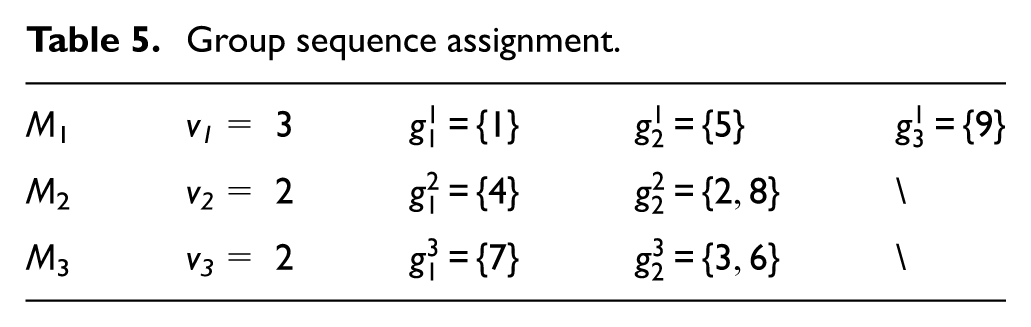
To illustrate the GS schedule, let us consider the example described in Section “Problem statement” and the corresponding groups of operation assignments given in Table 5. The disjunctive graph associated with the GS schedules is shown in Figure 4. This graph is an induced subgraph of the disjunctive graph given in Figure 1.

Table 5.

Group sequence assignment.

M ₁	v ₁= 3	$g_{1}^{1}$ = {1}	$g_{2}^{1}$ = {5}	$g_{3}^{1}$ = {9}
M ₂	v ₂= 2	$g_{1}^{2}$ = {4}	$g_{2}^{2}$ = { $2, 8$ }	\
M ₃	v ₃= 2	$g_{1}^{3}$ = {7}	$g_{2}^{3}$ = { $3, 6$ }	\

Figure 4.

GS disjunctive graph highlighting two-operation permutable groups.

Table 5 shows the sequence of groups for each machine. For M₁, we have three single-operation groups (i.e. v₁= 3) in this order: $g_{1}^{1} = {1}$ , $g_{1}^{2} = {5}$ , and $g_{1}^{3} = {9}$ , meaning that only one sequence is characterized, that is, ( $1, 5, 9$ ). For M₂, we have two groups (i.e. v₂=2) with $g_{2}^{1} = {4}$ sequenced before $g_{2}^{2} = {2, 8}$ , where operations 2 and 8 can be processed in any order; two sequences can then be characterized, which are (1, 2, 8) and (1, 8, 2). For M₃, we also have two groups (i.e. v₃=2): $g_{3}^{1} = {7}$ comes before $g_{3}^{2} = {3, 6}$ , where operations 3 and 6 are also interchangeable. The GS disjunctive graph of Figure 4 illustrates the solution given in Table 5 where the groups $g_{2}^{2}$ and $g_{3}^{2}$ are represented by the pair of red arcs. Four possible schedules are in Figure 5.

Figure 5.

Feasible schedules: (a) C_max= 4, (b) C_max= 4, (c) C_max= 4, and (d) C_max= 5.

As we can see, all operations within the group $g_{2}^{2}$ (respectively, $g_{2}^{3}$ ) can be permuted without violating the feasibility of the solutions.

It is important to note that each solution has its own makespan value, which allows us to evaluate the performance of the set of feasible schedules in the worst case by ${\bar{C}}_{\max} = 5$ (Figure 5(d)), while the optimal solution is known to be $C_{\max}^{*} = 4$ .

Decision support indicators

To fully benefit from the GS technique, it is imperative to evaluate the GS schedule once it has been generated by measuring its quality. Quality can be provided by a performance measure based on job completion times. Hence, the worst performance of a group is represented by its worst completion time. On the other hand, the best-case quality is also interesting to evaluate, and we will determine it by evaluating the best completion time of any job. At least, an indicator of flexibility allows us to measure the quality of the set of possible solutions that the GS technique characterizes.

Worst performance

The worst-case scenario evaluates the quality of GS by representing the worst-case scenario. To calculate it in a disjunctive graph, it is necessary to compute the maximum starting/completion times of the operations present in the set of feasible schedules described by a GS using the dynamic program given in Artigues et al.²⁴ The first step consists of determining the earliest worst-case starting time ${\bar{S}}_{i}$ for each i operation, considering the latest completion time of previous operations, and taking the maximum of these values. The operations preceding i include the operations in $(g^{-} (i))$ , as well as the predecessors $(Γ^{-} (i))$ of the operation i. The value of ${\bar{S}}_{i}$ therefore corresponds to the maximum between the release date of operation i, and the maximum of the worst-case completion times of the predecessors of the task i as given in equation (4).

{\bar{S}}_{i} = \max (r_{i}, \max_{j \in Γ^{-} (i) \cup g^{-} (i)} {\bar{C}}_{j})

(4)

The second step aims to calculate the worst-completion time ${\bar{C}}_{i}$ of the operation i. Two scenarios are possible: either i is executed first in its group, or another operation j in the group g(i), different from i and having the highest worst-earliest starting time, is executed first, while i is executed last. This is given by:

{\bar{C}}_{i} = \max ({\bar{S}}_{i} + p_{i}, \max_{j \in g (i), j \neq i} {\bar{S}}_{j} + \sum_{j \in g (i), j \neq i} p_{j} + p_{i})

(5)

Finally, the worst performance of the GS is given by: ${\bar{C}}_{\max} = \max {\bar{C}}_{i}$ .

As an application of equation (5) on the example Figure 2, we obtain ${\bar{C}}_{1} = 1, {\bar{C}}_{2} = 3, {\bar{C}}_{3} = 5, {\bar{C}}_{4} = 1, {\bar{C}}_{5} = 2, {\bar{C}}_{6} = 5, {\bar{C}}_{7} = 1, {\bar{C}}_{8} = 3$ , and ${\bar{C}}_{9} = 4$ . The worst performance is reached if operation 8 is executed first in $g_{2}^{2}$ and operation 3 executed first in $g_{2}^{3}$ , with ${\bar{C}}_{\max} = 5$ .

Best performance

In this section, we propose to evaluate the quality of a group in the best-case scenario or the most favorable scenario. In other words, we seek to determine for each group its best starting time, that is, the best starting time of each task belonging to the group.

Proposition 4. Given a task $i \in g_{k}^{l}$ and its predecessor $(i - 1)$ according to the product process, the best starting time of i is given by $S_{i} = \max (r_{i}, {\bar{C}}_{i - 1} - \sum_{j \in g (i - 1)} p_{j}, \max_{j \in g^{-} (i)} {\bar{C}}_{j}$ ) with ${\bar{C}}_{j}$ as given in equation (5).

Proof. We know that the temporal position of a task $i \in g (i)$ depends on the tasks that must precede it, that is, the tasks that belong to $Γ^{-} (i)$ and those that belong to $g^{-} (i)$ . However, we highlight that we are interested in the temporal position of i that allows performing it as soon as possible. Hence, it is obvious that the task i is processed earlier (best starting time) if all its predecessors in $\in Γ^{-} (i)$ are processed earlier. This can be achieved by sequencing any task j in its first position and not after all the other tasks in g(j) as given for the worst case. This explains the second term given in the formula of $S_{i}$ , that is, an adjustment of the worst-case completion time by subtracting the processing time of the other tasks in a group, except for the considered task in question. On the other hand, a task i is preceded by the tasks in $g^{-} (i)$ , and this justifies the third term given in the formula of $S_{i}$ .

We notice that, for determining the best performance and for purposes of simplification, we have maintained the same notation ${\bar{C}}_{j}$ , as we have used the equation (5), but its values, in this case, give the best completion time.

Proposition 5. The job, such as $j^{*} = argma x_{j = 1 . . . n} ({\underline{S}}_{n_{j^{*}}} + p_{n_{j}^{*}}$ ) is a lower bound for the problem $J | p_{i} = p | C_{\max}$ with a completion time noted ${\underline{C}}_{\max} = \max ({\underline{S}}_{i} + p_{i})$ .

Proof. Evident.

If we consider again our reference example, the best finishing time of each operation is: ${\underline{C}}_{1} = {\underline{C}}_{4} = {\underline{C}}_{7} = 1, {\underline{C}}_{2} = {\underline{C}}_{5} = 2, {\underline{C}}_{8} = 2, {\underline{C}}_{3} = {\underline{C}}_{6} = 3$ , and ${\underline{C}}_{9} = 4$ . It is the third job who defines the best performance with $\underline{C_{\max}} = {\underline{C}}_{9} = 4$

Sequential flexibility

As previously stated, GS characterizes a set of feasible schedules without listing them, ensuring sequential flexibility. An evaluation of this set is required and is considered a measure of flexibility. In this context, there are two measures for GS schedules presented in Esswein.²² This concerns the total number of groups contained in a solution and designated by $# Gps = \sum_{k = 1, \dots, v_{ℓ}}^{l = 1, \dots, m} g_{k}^{ℓ}$ , and the number of sequences characterized by the groups given by $# Seq = Π_{k = 1, \dots, v_{ℓ}}^{l = 1, \dots, m} (| g_{k}^{ℓ} |!)$ . Another metric introduced in Artigues et al.²⁴ and denoted by φ is given by equation (6) measures the ratio between the number of groups $# Gps$ and the size of the problem $n \times x m$ .

φ = \frac{(n \times m) - # Gps}{(n \times m) - m} \times 100 %

(6)

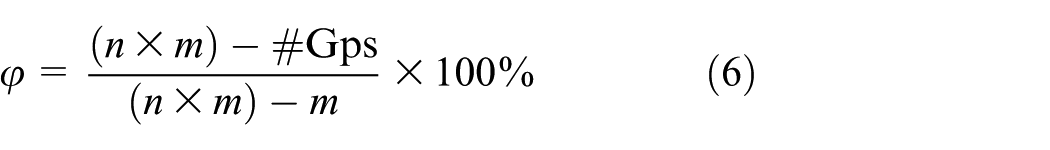
As we can see from the formula, when the number of groups is equal to the number of operations, the flexibility is minimal ( $φ = 0 %$ ). Whereas if all operations of each machine constitute a single group, the flexibility is maximal ( $φ = 100 %$ ; Table 6).

Table 6.

Lower bound computations for the example given in Figure 1.

$J_{n}$	J ₁			J ₂			J ₃
O _i	1	2	3	4	5	6	7	8	9
$g^{-} (i)$	\	{4}	{7}	\	{1}	{7}	\	{4}	{5}
$g (i - 1)$	\	{1}	${2, 8}$	\	{4}	{5}	\	{7}	${2, 8}$
r _i	0	1	2	0	1	2	0	1	2
${\bar{C}}_{i - 1} - \sum_{j \in g (i - 1)} p_{j}$	0	1	2	0	1	2	0	1	3
$\max_{j \in g^{-} (i)} {\bar{C}}_{j}$	0	1	1	0	1	1	0	1	2
$S_{i}$	0	1	2	0	1	2	0	1	3

Among these indicators, $# Seq$ might seem more significant because it more fully represents sequential flexibility. However, because it can quickly reach extremely high values, it would be difficult to interpret it. To this end, we have introduced new flexibility metrics that measure the minimum and maximum sequence numbers relative to a machine, which are given by: $\underline{Seq} = mi n_{l = 1 . . . m} (\underset{k = 1, \dots, v_{l}}{Π} (| g_{k}^{l} |!))$ and $\bar{Seq} = ma x_{l = 1 . . . m} (\underset{k = 1, \dots, v_{l}}{Π} (| g_{k}^{l} |!))$ .

For our example in Figure 3, $φ = 2 / 6 = 33.33 %$ , $\underline{Seq}$ = 1 (defined for M1) and $\bar{Seq}$ = 2!× 1! = 2 (defined for machines M2 or M3).

To illustrate the principle of the proposed approach in handling unanticipated events during the reactive phase. Let us consider the example given in Table 5 with an unexpected event (e.g. arrival of an urgent task or a maintenance activity). We suppose that the unexpected task u occurs at time t= 2 with a processing time p_u= 1 and needs to be performed on machine M₃. The set of tasks {1, 4, 5, 7, 8} has been completed. We know a priori that set {3, 6} is a group of permutable operations and $\bar{S_{3}} = \bar{S_{4}} = 4$ . The decision-maker can then position the task u just before the group with a stating time s_u= 2 and a finishing time c_u= 3 with the guarantee that the performance will not be degraded. In other words, the schedule remains feasible with ${\bar{C}}_{\max} = 5$ since the starting time $S_{3} \leq \bar{S_{3}}$ and $S_{6} = \bar{S_{4}} \leq 4$ (see Figure 6).

Figure 6.

Illustration of the generality of the proposed approach through urgent task scenario on M₃.

This scenario demonstrates that the proposed method can effectively handle real-time disruptions without violating precedence constraints or increasing the worst-case makespan. The flexibility that fully permutable groups bring allows preserving schedule feasibility and makes the approach both robust and applicable to dynamic environments.

Computational experiments

All the numerical experiments were conducted on a personal computer equipped with an Intel Core i5-4210U CPU @ 1.70 GHz, 4 GB RAM, and Windows 10 (64-bit). All algorithms were implemented in C++ and compiled with g++ (TDM-GCC 9.2.0) in single-thread mode using the -O3 optimization flag. To evaluate our approach, we have conducted extensive computational tests on a set of instances obtained from the job-shop OR-library (https://people.brunel.ac.uk/∼mastjjb/jeb/orlib/files/jobshop1.txt). This library offers sets of square instances: La01-La40 (Lawrence), orb01-orb10 (Applegate and Cook), and ft06, ft10, ft20 (Fisher and Thompson), as well as the modified sets abz05m-abz09m (Adams, Balas, and Zawack) and yn01m-yn04m (Yamada and Nakano), covering various workshop planning scenarios. In order to adapt these benchmarks to our problem, we fixed the processing time for each task i to one unit p_i= 1.

For each benchmark instance, a feasible solution is first generated using Algorithm 1. Its runtime is not included in reported computational times. The CPU time refers exclusively to the adapted EBJG grouping procedure and to the computation of the lower bound. We specify that the original EBJG runs in polynomial time,²² and the additional condition introduced to the adapted version of our approach does not change the overall complexity of the algorithm, as it only adds, at each iteration, a constant-time for checking. Moreover, the algorithm stops when no more operations satisfy the grouping condition or when the worst-case schedule reaches the maximum deviation (D = 20%) allowed from the makespan of the initial solution. The purpose is to preserve sequential flexibility while controlling the performance degradation.

The experimental results are summarized in Tables 7 to 11. We assigned the notation $n \times x m$ to each instance, where n and m represent, respectively, the number of jobs and machines.

Table 7.

Test results for La01m-La40m instances.

nXm	Instances	$L b^{(k)}$	Lb _n	$U b^{(k)}$	${\bar{C}}_{\max}$	D1	D2	$# Gps$	φ (%)	$\underline{Seq}$	$\bar{Seq}$	CPU
10 × 5	La01	10	10	10	13	0.30	0.30	25	56	12	864	0.578
	La02	11	11	11	14	0.27	0.27	27	51	16	720	0.625
	La03	12	12	12	14	0.17	0.17	29	47	4	4320	0.985
	La04	11	11	11	13	0.18	0.18	28	49	8	144	0.610
	La05	10	$11^{+}$	11	14	0.27	0.27	22	62	8	1440	0.562
15 × 5	La06	15	15	15	19	0.27	0.27	38	53	96	69,210	0.859
	La07	16	16	16	20	0.25	0.25	34	59	96	518,400	0.906
	La08	15	15	15	17	0.13	0.13	34	59	48	34,560	0.859
	La09	15	15	15	16	0.07	0.07	33	60	144	181,440	0.906
	La10	16	16	16	18	0.13	0.13	35	57	576	6912	0.875
20 × 5	La11	21	21	21	25	0.19	0.19	37	66	864	$9, 2 \times 10^{7}$	1.140
	La12	20	20	20	22	0.10	0.10	38	65	3456	$3, 8 \times 10^{8}$	1.560
	La13	20	20	20	23	0.15	0.15	33	71	5184	$1, 7 \times 10^{8}$	1.171
	La14	20	20	20	23	0.15	0.15	34	70	720	$4, 9 \times 10^{6}$	1.046
	La15	20	20	20	26	0.30	0.30	37	66	5760	$4, 2 \times 10^{6}$	1.234
10 × 10	La16	13	$15^{+}$	16	21	0.40	0.31	73	30	2	96	0.981
	La17	15	15	15	19	0.27	0.27	67	37	2	72	1.140
	La18	14	14	15	21	0.50	0.40	67	37	2	288	1.312
	La19	15	15	15	20	0.33	0.33	74	29	2	288	1.140
	La20	14	14	15	19	0.36	0.27	73	30	2	16	1.203
15 × 10	La21	18	18	20	25	0.39	0.25	99	36	8	960	1.750
	La22	18	18	19	26	0.44	0.37	103	33	2	1152	1.727
	La23	17	17	18	26	0.53	0.44	99	36	8	576	1.782
	La24	17	17	18	22	0.29	0.22	99	36	4	1440	1.844
	La25	18	18	19	28	0.56	0.47	106	31	4	5760	1.766
20 × 10	La26	22	22	23	25	0.14	0.09	115	45	96	23,040	2.400
	La27	22	22	24	29	0.32	0.21	118	43	128	37,560	2.280
	La28	22	22	22	27	0.23	0.23	116	44	48	69,120	2.327
	La29	21	21	24	31	0.48	0.29	115	45	96	69,120	2.290
	La30	21	21	24	30	0.43	0.25	129	37	96	5184	2.359
30 × 10	La31	32	32	32	38	0.19	0.19	152	51	9216	$9, 9 \times 10^{7}$	3.484
	La32	31	31	32	37	0.19	0.16	145	53	8547	$7, 3 \times 10^{7}$	3.498
	La33	30	30	32	39	0.30	0.22	147	53	13,824	$4, 9 \times 10^{7}$	3.469
	La34	31	$32^{+}$	32	37	0.19	0.16	161	48	6144	$5, 9 \times 10^{7}$	3.422
	La35	30	30	32	42	0.40	0.31	157	39	2304	$5, 1 \times 10^{7}$	3.578
15 × 15	La36	18	$21^{+}$	23	28	0.33	0.22	152	35	4	1440	2.562
	La37	22	22	24	27	0.23	0.13	145	38	2	644	2.428
	La38	20	$21^{+}$	23	30	0.43	0.30	147	37	4	348	2.766
	La39	20	20	23	26	0.30	0.13	147	37	2	420	2.650
	La40	20	$21^{+}$	25	28	0.33	0.12	134	44	2	720	2.391
Average						0.29	0.23	85.6	47			1.762

Table 8.

Test results for abz05m-abz09m instances.

nXm	Instances	$L b^{(k)}$	Lb _n	$U b^{(k)}$	${\bar{C}}_{\max}$	D1	D2	$# Gps$	φ %	$\underline{Seq}$	$\bar{Seq}$	CPU
10 × 10	abz05	13	$14^{+}$	15	19	0.46	0.27	72	31	2	120	0.996
	abz06	24	24	27	28	0.17	0.19	68	35	4	240	0.991
20 × 15	abz07	24	24	27	32	0.33	0.19	198	36	8	5760	2.964
	abz08	24	$25^{+}$	27	34	0.42	0.26	199	35	8	69,120	3.861
	abz09	24	24	28	34	0.42	0.21	198	36	8	23,040	3.254
Average						0.36		147	34			2.413

Table 9.

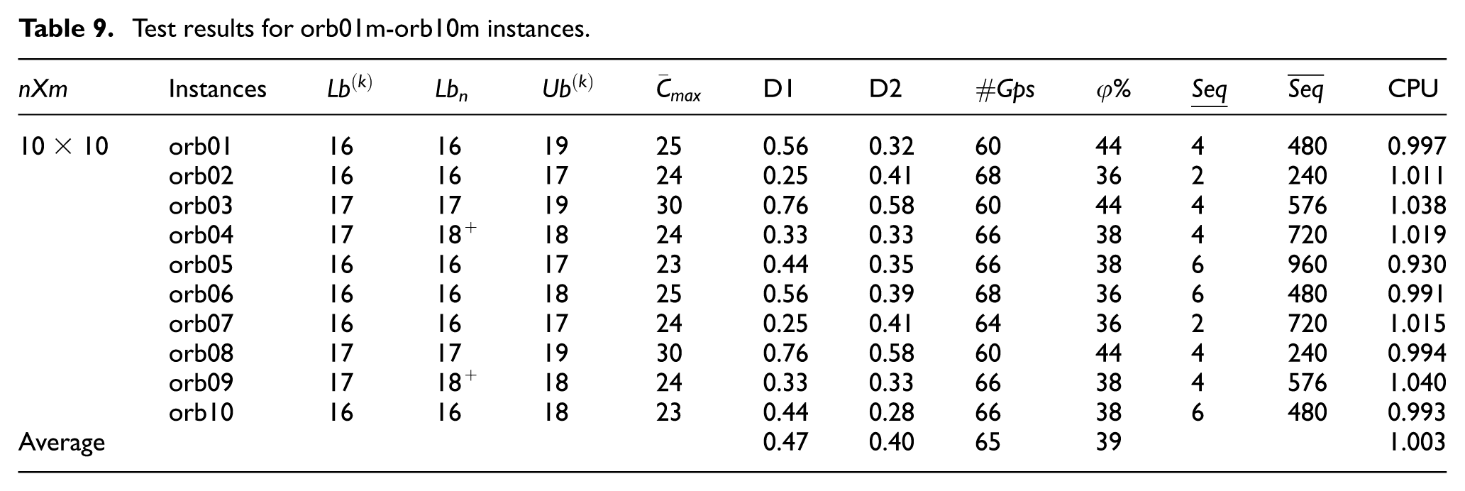
Test results for orb01m-orb10m instances.

nXm	Instances	$L b^{(k)}$	Lb _n	$U b^{(k)}$	${\bar{C}}_{\max}$	D1	D2	$# Gps$	φ%	$\underline{Seq}$	$\bar{Seq}$	CPU
10 × 10	orb01	16	16	19	25	0.56	0.32	60	44	4	480	0.997
	orb02	16	16	17	24	0.25	0.41	68	36	2	240	1.011
	orb03	17	17	19	30	0.76	0.58	60	44	4	576	1.038
	orb04	17	$18^{+}$	18	24	0.33	0.33	66	38	4	720	1.019
	orb05	16	16	17	23	0.44	0.35	66	38	6	960	0.930
	orb06	16	16	18	25	0.56	0.39	68	36	6	480	0.991
	orb07	16	16	17	24	0.25	0.41	64	36	2	720	1.015
	orb08	17	17	19	30	0.76	0.58	60	44	4	240	0.994
	orb09	17	$18^{+}$	18	24	0.33	0.33	66	38	4	576	1.040
	orb10	16	16	18	23	0.44	0.28	66	38	6	480	0.993
Average						0.47	0.40	65	39			1.003

Table 10.

Test results for yn01m-yn04m instances.

nXm	Instances	$L b^{(k)}$	Lb _n	$U b^{(k)}$	${\bar{C}}_{\max}$	D1	D2	$# Gps$	φ%	$\underline{Seq}$	$\bar{Seq}$	CPU
20 × 20	yn01	24	$27^{+}$	30	39	0.44	0.30	297	27	4	5760	4.123
	yn02	25	$27^{+}$	31	36	0.33	0.16	284	31	16	10,368	4.095
	yn03	27	$28^{+}$	32	37	0.37	0.15	297	27	2	1152	3.857
	yn04	28	28	34	39	0.39	0.14	292	28	8	1728	3.937
Average						0.39	0.19	293	28			4.003

Table 11.

Test results for ft06m, ft10m, and ft20m instances.

nXm	Instances	$L b^{(k)}$	Lb _n	$U b^{(k)}$	${\bar{C}}_{\max}$	D1	D2	$# Gps$	φ%	$\underline{Seq}$	$\bar{Seq}$	CPU
6 × 6	ft06	8	8	9	11	0.38	0.22	25	36	2	12	0.358
10 × 10	ft10	16	16	18	27	0.69	0.50	62	42	4	720	1.117
20 × 5	ft20	22	22	24	35	0.59	0.38	37	66	4608	$4, 8 \times 10^{8}$	0.918
Average						0.55	0.37	41	48			0.798

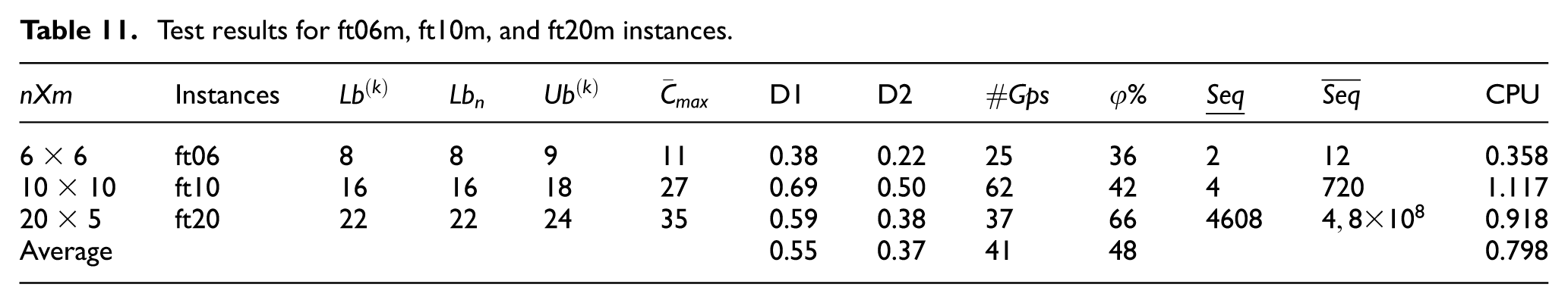
In the following, we compare our lower bounds Lb_n with the best results $L b^{(k)}$ proposed in Kouider et al.¹⁰ The column labeled ${\bar{C}}_{\max}$ reports the worst performance of the group solutions resulting from the modified EBGJ method. The metric (D1) quantifies the relative difference between the worst makespan and our lower bound using the formula $D 1 = \frac{{\bar{C}}_{\max} - L b_{n}}{L b_{n}}$ , while the metric (D2) quantifies the relative difference between the worst makespan and the upper bound defined in Kouider et al.¹⁰ using the formula $D 2 = \frac{{\bar{C}}_{\max} - U b^{(k)}}{U b^{(k)}}$ . The column $# Gps$ lists the number of groups resulting from our approach, followed by φ which measures the proportion $# Gps$ relative to the size of the instance. The column $\underline{Seq}$ (resp. $\bar{Seq}$ ) indicates the minimum (resp., maximum) number of alternative sequences characterized for one machine among all machines of the instance. Finally, the last column indicates the running CPU time of our approach (in seconds).

Based on the results presented in the five tables, we compare our lower bound that represents the best completion of any job when it is performed earlier (in the best case defined by the partial order given by our adapted EBJG approach) to the Lb_n value proposed in the literature. For all instances, our bounds are either equal to $L b^{(k)}$ or better than $L b^{(k)}$ for 13 instances (⁺).

It should be mentioned that the presence of a gap between the upper and lower bounds motivates new research efforts so that instances that have not yet been resolved converge toward optimal solutions. As part of our work, our contribution goes in this direction. Indeed, some of our lower bounds Lb_n, when they are not equal to those given in the literature, are much tighter and thus improve the quality of the solutions. For example, for instance Y04, our lower bound Lb_n, equal to 28, corresponds to the literature value $L b^{k}$ , with an upper bound $U b^{k}$ equal to 34, thus confirming the complexity of the instance. Unlike, for instance Y01, where Lb_n is equal to 27, exceeding thus $L b^{k}$ which is equal to 24, when knowing that $U b^{k}$ is equal to 30. We clearly notice that the gap has been reduced from 6 to 3, which demonstrates the relevance of our approach. Moreover, we emphasize that the interpretation of our lower bound is quite specific. It represents the biggest makespan value of a job sequence among the group’s job sequences when the operations of this job are all scheduled as early as possible; the other jobs can be scheduled at their worst-case positions.

The performance of our approach is evaluated using the two measures (D1) and (D2), which allow us to compare our worst performance ( ${\bar{C}}_{\max}$ ) with our lower bound on the one hand and the upper bound from the literature on the other, as well as the flexibility measures. If we focus on (D2), we notice that our results deviate between $19 %$ and $40 %$ compared to the known solutions (unique solution) but with a sequential flexibility (set of solutions) given by φ in a range that varies from $28 %$ to $48 %$ . It should be noted, quite obviously, that the higher the $# Gps$ , the lower the φ. It should also be mentioned that the higher $\bar{Seq}$ is, the higher is $\underline{Seq}$ , according to the various results found. However, no conclusion can be drawn regarding the correlation between the two pairs of indicators, as it depends on the nature of the instance.

Conclusion

This paper considered robust JSSP with unit processing times. Our goal was to design a set of solutions rather than a single solution capable of adapting to unforeseen events that could disrupt the production system, leveraging the flexibility provided. To achieve this, we applied two complementary methods, which we adapted to our specific problem: a heuristic approach to generate a schedule having a specific interval structure and allowing to apply a GS method and hence create groups of fully interchangeable operations, with a performance evaluated in the best and worst scenarios. The computational results using benchmarks from OR-Library and adapted to our studied problem have shown, on one hand, the good quality of the proposed lower bound, which is equivalent to sequencing a job in the best case. On the other hand, the results obtained on worst-case performance compared to the generated flexibility validate the relevance of our approach, which aims to anticipate environmental disturbances.

Scheduling problems with unit processing times are widely studied in the literature because they offer both theoretical and practical contributions. The JSSP remains NP-hard in this case and demonstrates its inherent computational difficulty. When the application environment is uncertain, models developed serve as standard references for evaluating the performance of planning algorithms, particularly approximation or heuristic methods. The proposed approach is a contribution to this field because it offers multiple schedules instead of a single solution, allowing a group of operations to be completely permutable, thus ensuring sequential flexibility. The current method is particularly well tailored for instances with equal processing times where operations share identical release and due dates on the same machine. Our lower bound surpasses some results in the literature; moreover, it can be generalized for the case where the processing times are arbitrary in future research.

For future research, it would also be interesting to integrate the proposed approach into a real-life decision support system, taking into account the influence of the human factor. An application of this kind would verify and enhance the theoretical results by testing the robustness of the approach in contexts where human decisions play a central role.

Footnotes

Handling Editor: Chenhui Liang

ORCID iDs

Sara Bouguessa

Samia Ourari

Funding

The authors received no financial support for the research, authorship, and/or publication of this article.

Declaration of conflicting interests

The authors declared no potential conflicts of interest with respect to the research, authorship, and/or publication of this article.

References

Chuang

Guanghui

Junsheng

Smart cyber-physical production system enabled workpiece production in digital twin job shop. Adv Mech Eng 2021; 13(9): 16878140211040888.

Caldeira

Gnanavelbabu

Vaidyanathan

An effective backtracking search algorithm for multi-objective flexible job shop scheduling considering new job arrivals and energy consumption. Comput Ind Eng 2020; 149: 106863.

Sun

Xiao

Risk measure of job shop scheduling with random machine breakdowns. Comput Oper Res 2018; 99: 1–12.

Wang

Cheng

Liu

, et al. Multi-objective reinforcement learning framework for dynamic flexible job shop scheduling problem with uncertain events. Appl Soft Comput 2022; 131: 109717.

Luo

Gong

Knowledge-driven two-stage memetic algorithm for energy-efficient flexible job shop scheduling with machine breakdowns. Expert Syst Appl 2024; 235: 121149.

Afsar

Palacios

Puente

, et al. Multi-objective enhanced memetic algorithm for green job shop scheduling with uncertain times. Swarm Evol Comput 2022; 68: 101016.

Zhou

Zhu

Tang

, et al. Reinforcement learning for online optimization of job-shop scheduling in a smart manufacturing factory. Adv Mech Eng 2022; 14(3): 16878132221086120.

Xiong

Fan

Taghipour

Research on steady-state simulation in dynamic job shop scheduling problem. Adv Mech Eng 2015; 7(9): 1687814015604546.

Wan

Mei

Two-agent scheduling of unit processing time jobs to minimize total weighted completion time and total weighted number of tardy jobs. Eur J Oper Res 2021; 290: 26–35.

10.

Kouider

Haddadene

Ourari

, et al. Mixed graph colouring for unit-time scheduling. Int J Prod Res 2016; 55(6): 1720–1729.

11.

Ghaleb

Zolfagharinia

Taghipour

Real-time production scheduling in the Industry-4.0 context: addressing uncertainties in job arrivals and machine breakdowns. Comput Oper Res 2020; 123: 105031.

12.

Zhou

Zhang

Sarker

, et al. An event-triggered dynamic scheduling method for randomly arriving tasks in cloud manufacturing. Int J Comput Integr Manuf 2018; 31(4): 318–333.

13.

Zhang

Zhou

Peng

, et al. Dynamic flexible job shop scheduling method based on improved gene expression programming. Meas Control 2020; 54(7–8): 1136–1146.

14.

Zhang

Buchmeister

An efficient metaheuristic algorithm for job shop scheduling in a dynamic environment. Mathematics 2023; 11(10): 2336.

15.

Qiu

Sawhney

Zhang

, et al. Data mining–based disturbances prediction for job shop scheduling. Adv Mech Eng 2019; 11(3): 1687814019838178.

16.

Wang

Xie

HX.

Bad-scenario-set robust scheduling for a job shop to hedge against processing time uncertainty. Int J Prod Res 2019; 57(11): 3168–3185.

17.

Wang

Liu

Jin

A proactive scheduling approach to steel rolling process with stochastic machine breakdown. Nat Comput 2019; 18(4): 679–694.

18.

Xiao

Dui

Resilience-based surrogate robustness measure and optimization method for robust job-shop scheduling. Mathematics 2022; 10(21): 4048.

19.

Grumbach

Müller

Reusch

Robustness prediction in dynamic production processes—a new surrogate measure based on regression machine learning. Processes 2023; 11(4): 1267.

20.

Davari

Demeulemeester

The proactive and reactive resource-constrained project scheduling problem. J Sched 2019; 22: 211–237.

21.

Billaut

Roubella

A new method for workshop real time scheduling. Int J Prod Res1996; 34: 1555–1579.

22.

Esswein

Un apport de flexibilité séquentielle pour l’ordonnancement robuste. PhD Thesis, Tours University, France, 2003.

23.

Pinot

Coopération homme-machine pour l’ordonnancement sous incertitudes. PhD Thesis, Université de Nantes, France, 2008.

24.

Artigues

Billaut

Esswein

Maximization of solution flexibility for robust shop scheduling. Eur J Oper Res 2005; 165: 314–328.

25.

Artigues

Billaut

Cherif

, et al. Robust machine scheduling based on group of permutable jobs. In: Doumpos

Zopounidis

Grigoroudis

(eds) Robustness analysis in decision aiding, optimization, and analytics. International Series in Operations Research and Management Science. Springer, 2016, pp.191–220.

26.

Aloulou

Artigues

Flexible solutions in disjunctive scheduling: general formulation and study of the flow-shop case. Comput Oper Res 2010; 37(5): 890–898.

27.

Erschler

Fontan

Mercé

, et al. A new dominance concept in scheduling n jobs on a single machine with ready times and due dates. Oper Res 1983; 31(1): 114–127.

28.

Briand

Erschler

A robust approach for the single machine scheduling problem. J Sched 2007; 10(3): 209–221.

29.

Erschler

Roubellat

An approach for real time scheduling for activities with time and resource constraints. In: Slowinski

Weglarz

(eds) Advances in project scheduling. Elsevier, 1989, pp.237–272.

30.

Oron

Shabtay

Steiner

Single machine scheduling with two competing agents and equal job processing times. Eur J Oper Res 2015; 244(1): 86–99.

31.

Lazarev

Arkhipov

Werner

Scheduling jobs with equal processing times on a single machine: minimizing maximum lateness and makespan. Optim Lett 2017; 11: 165–177.

32.

Chen

Geng

, et al. Pareto-scheduling of two competing agents with their own equal processing times. Eur J Oper Res 2022; 301(2): 414–431.

33.

Shen

Liang

Faster algorithms for bicriteria scheduling of identical jobs on uniform machines. J Ind Manag Optim 2023; 19(7): 5398–5406.

34.

Kravchenko

Werner

Parallel machine problems with equal processing times: a survey. J Sched 2011; 14: 435–444.

35.

van Bevern

Pyatkin

. Completing partial schedules for open shop with unit processing times and routing. In: Kulikov

Woeginger

(eds) Computer science – theory and applications. CSR 2016. Lecture Notes in Computer Science, vol 9691. Springer, 2016, pp.73–87.

36.

Shabtay

Karhi

Online scheduling of two job types on a set of multipurpose machines with unit processing times. Comput Oper Res 2012; 39(2): 405–412.

37.

Chen

Liu

, et al. Online scheduling with unit processing times and processing set restrictions. J Oper Res Soc China 2019; 7(3): 475–484.

38.

Sotskov

Mihova

EI.

Scheduling multiprocessor tasks with equal processing times as a mixed graph coloring problem. Algorithms 2021; 14(8): 246.

39.

Sotskov

Dolgui

Werner

. Optimal coloring of the vertices from the unions of paths and cliques. In: Discrete optimization methods in scheduling and computer-aided design, Minsk, Belarus, 5–6 September 2000, pp.93–98. Minsk: National Academy of Sciences of Belarus.

40.

Sotskov

YN.

Mixed graph colorings: a historical review. Mathematics 2020; 8(3): 385.

41.

Kouider

Haddadene

HA.

A bi-objective branch-and-bound algorithm for the unit-time job shop scheduling: a mixed graph coloring approach. Comput Oper Res 2021; 132: 105319.

42.

Lenstra

Rinnooy Kan

AHG

Brucker

Complexity of machine scheduling problems. Ann Discrete Math 1977; 1: 343–362.

43.

Roy

Sussmann

Les problèmes d’ordonnancement avec contraintes disjonctives. Research report, SEMA, 1964.

44.

Esquirol

Lopez

L’ordonnancement. Economica, 1999.

45.

Adams

Balas

Zawack

The shifting bottleneck algorithm for job-shop scheduling. Manage Sci 1988; 34: 391–401.

46.

Allen

JF.

Time and time again: the many ways to represent time. Int J Intell Syst 1991; 6(4): 341–355.

47.

Ourari

Berrandjia

Boulakhras

, et al. Robust approach for centralized job shop scheduling: sequential flexibility. IFAC Pap OnLine 2015; 48(3): 1960–1965.

48.

Billaut

Moukrim

Sanlaville

Flexibility and robustness in scheduling. Wiley-ISTE, 2008.

49.

Cardin

Mebarki

Pinot

A study of the robustness of the group scheduling method using an emulation of a complex FMS. Int J Prod Econ 2013; 146(1): 199–207.

50.

Yahouni

Mebarki

Belkadi

, et al. Human-machine cooperation in planning and scheduling: a case study on an unstable environment. Eur J Ind Eng 2018; 12(6): 757–764.

51.

Yahouni

Le meilleur des cas pour l’ordonnancement de groupes : Un nouvel indicateur proactif-réactif pour l’ordonnancement sous incertitudes. Automatique. École Centrale de Nantes, Université Abou Bekr Belkaid, Tlemcen, Algérie, 2017.

Job shop scheduling with unit processing times under uncertainties: Sequential flexibility and new lower-bound

Abstract

Keywords

Introduction

Literature review

Scheduling under uncertainty

Scheduling problem with unit processing times

Problem statement

Problem decomposition and dominant sequences

Local scheduling

Interval structure and dominance principle

Propriety of the JSSP with equal processing times

Global scheduling

Group sequence based approach

Generation of group sequence schedules: An adapted EBJG

Example illustration

Decision support indicators

Worst performance

Best performance

Sequential flexibility

Computational experiments

Conclusion

Footnotes

ORCID iDs

Funding

Declaration of conflicting interests

References