Sage Journals: Discover world-class research

Abstract

With the annual increase in car ownership, traffic congestion and related issues are becoming increasingly severe. Urban traffic flow exhibits time-varying and stochastic characteristics, presenting a major challenge for prediction. Most existing prediction models require manual tuning of hyperparameters, which is often complex, lacks global optimality, and is prone to overfitting. Therefore, this paper applies the CAPSO algorithm to the traditional BP neural network, integrating chaotic mapping to enhance population diversity. It employs adaptive parameter balancing for exploration and development, thereby avoiding convergence to local optima. Additionally, it iterates the relevant parameters of the neural network to identify the global optimal value. The BP neural network for short-term traffic flow prediction at road intersections has been optimized and refined, resulting in a significant improvement in prediction accuracy. The linear correlation has increased by 9.23% compared to the previous BP neural network. Additionally, the speed of iterative convergence has been greatly enhanced, and the sensitivity to initial weights has been substantially reduced. These improvements contribute to a prediction model that demonstrates greater accuracy, timeliness, and robustness. This model can be utilized to optimize traffic management, providing essential data support for enhancing traffic efficiency and contributing to the development of smart cities.

Keywords

urban traffic flow prediction BP neural network PSO algorithm CAPSO algorithm chaotic perturbation

Introduction

With the rapid development of the economy, motor vehicles have become one of the most important modes of transportation in people’s daily lives. The demand for automobiles has grown increasingly strong. According to data from the China Association of Automobile Manufacturers (CAAM), China’s automobile production and sales in 2024 totaled 31.282 and 31.436 million units, representing year-on-year growth of 3.7% and 4.5%, respectively. This significant increase in the number of cars will inevitably lead to a rapid rise in traffic flow and increasingly severe issues such as traffic congestion. These problems not only affect the efficiency of daily travel but also exacerbate air pollution, diminish the quality of life for urban residents, and pose threats to economic development and social stability in cities. Therefore, accurately predicting traffic flow is essential to provide reliable data support for road traffic management. By rationally planning traffic flow based on this data, we can greatly enhance the operational efficiency of roadways and alleviate the aforementioned issues.¹

Traffic flow prediction can be categorized into short-term traffic flow prediction² and long-term traffic flow prediction. Short-term traffic flow prediction forecasts traffic conditions for the immediate future, typically the next moment or the next few minutes. This type of prediction is highly time-sensitive, allowing individuals to adjust their travel choices based on real-time traffic conditions, thereby facilitating efficient travel.³ In contrast, long-term traffic flow prediction focuses on extended timeframes, playing a crucial role in the optimization of urban road systems and traffic network planning.

Traffic management can be optimized to alleviate congestion through short-term traffic flow prediction. Real-time regulation of signal durations can be implemented based on traffic flow prediction data, thereby reducing queuing times at intersections and facilitating dynamic route guidance. Additionally, it can enhance tidal lane management.⁴ Predictive technology can minimize ineffective detours, resulting in fuel cost savings. Notably, following the implementation of the prediction system in the main urban area of Chongqing, the number of traffic accidents requiring police response in 2022 decreased by 18% year-on-year, leading to a reduction in direct economic losses of 120 million yuan. In the context of smart green city development, short-term traffic flow prediction can enhance speed efficiency across the city’s road network, support smart city initiatives, and promote environmental protection and emission reduction. Looking ahead, the deep integration of predictive technology with vehicle-road coordination and digital twin technology will empower the advancement of emerging technologies, making urban transport systems more adaptive and providing essential support for sustainable development.

Currently, numerous models and methods exist for traffic flow prediction, with neural network-based approaches being particularly favored by researchers. As a form of machine learning technology that emulates the neural networks of the human brain to achieve artificial intelligence-like capabilities, neural networks have been widely utilized in image recognition, language processing, data prediction, and other critical applications since their inception. This popularity is attributed to their powerful nonlinear fitting capabilities, strong generalization ability, robustness, fault tolerance, and parallel computing efficiency. Zaraket et al. proposed a hybrid traffic prediction model based on prophet model and long short-term memory neural network (LSTM), called Hyper-Flophet, to predict next traffic flow.⁵ This model adopts the traditional neural prophet model but with major parameter tuning. They proposed an efficient algorithm for predicting the traffic flow trend and developed an interactive LSTM (I-LSTM) model for auto-regression components. Xu and Gu proposed a prediction model based on adaptive multi-channel graph convolutional neural networks (AMGCN).⁶ The model utilizes an adaptive adjacency matrix to automatically learn implicit graph structures from data, introduces a mixed skip propagation graph convolutional neural network model, which retains the original node states and selectively acquires outputs of convolutional layers, thus avoiding the loss of node initial states and comprehensively capturing spatial correlations of traffic flow. Lieskovska et al. explored a Transformer-based model designed for traffic flow prediction,⁷ which integrates traditional time series values with derived time-related features, enhancing the model’s predictive capabilities. Liu and Zhang proposed an adaptive traffic flow prediction model AD-GNN based on spatiotemporal graph neural network.⁸ The gated temporal convolutional network captures the temporal dependence between layers. The diffusion graph convolutional network simulates the spatial relationship between nodes. Then, the parameterized adjacency matrix are used to construct an adaptive convolutional network to adaptively mine the implicit global deep spatial dependence. Zhao et al. proposed a multi-step trend aware graph neural network (MSTAGNN),⁹ which considers the influence of global spatiotemporal information and captures the dynamic characteristics of spatiotemporal graph. The experimental results shows that the model’s mean absolute error (MAE) is reduced by 6.25% and the total training time is reduced by 79%.

The existing neural network algorithm models, particularly LSTM deep network structure, are highly sensitive to initial weight settings. When training data is insufficient, the risk of encountering local optima increases, necessitating a substantial amount of data and computational resources to mitigate overfitting. In contrast, the chaotic adaptive particle swarm optimization (CAPSO) algorithm demonstrates greater stability with smaller datasets. In terms of parameter optimization, CAPSO can directly optimize network parameters, while LSTM’s hyper-parameters (e.g. learning rate, number of hidden layer nodes, etc.) need to be manually debugged, with higher complexity, which shows that back propagation (BP) neural network optimized by CAPSO is more efficient. The GNN model requires complex graph structure data and adjacency matrix definitions, whereas CAPSO only requires regular feature inputs (e.g. historical traffic flow, etc.), which is more broadly applicable. GNN has higher requirements on computational resources (e.g. GPU), while CAPSO can run efficiently on regular servers. CAPSO can be combined with traditional feature engineering (e.g. normalization, temporal feature extraction) and does not need to rely on spatial modeling of graph data. Compared with particle swarm optimization (PSO) algorithm, the chaotic perturbation strategy of CAPSO–BP accelerates the convergence speed and the adaptive mechanism reduces the ineffective search paths, which improves the convergence speed, accuracy, and avoids the local optimum. The performance is more stable in complex optimization problems. It can also avoid premature convergence and is suitable for high-dimensional, multi-peak optimization problems such as neural network parameter optimization.

CAPSO intricately combines chaotic mapping with swarm intelligence based on PSO. It employs a parameter adaptive adjustment mechanism and a dynamic hybrid optimization strategy to facilitate a smooth transition from global search during the initial iterations to local development in the later stages. This paper utilizes a BP neural network enhanced by CAPSO to predict short-term traffic flow during the evening peak hours at the intersection of Feicui Road and Danxia Road in Hefei City, Anhui Province, China. The testing set’s mean squared error (MSE)¹⁰ is reduced by 90.12% compared to the traditional BP neural network algorithm and by 83.80% compared to the PSO–BP algorithm, demonstrating superior accuracy and robustness.

Methods

BP neural network

As a multilayer feedforward neural network trained using the error back propagation algorithm, BP neural network is one of the most widely utilized neural network architectures. It is primarily divided into two components: forward propagation and back propagation.¹¹ During forward propagation, the predicted value is generated by sequentially calculating the output of each neuron layer through the weighted connections between neurons, progressing from the input layer to the output layer. In the back propagation phase, the error for each layer is computed based on the difference between the prediction value and the actual value. Subsequently, the network’s parameters are adjusted using gradient descent to minimize this error. This process is iterated multiple times until the network’s error falls below a specified threshold or other termination criteria are satisfied, indicating that the final result has been achieved.

BP neural network consists of an input layer, one or more hidden layers, and an output layer.¹² Each layer contains a specific number of nodes. Every node in a BP neural network comprises an input term $x_{i}$ , a weight $w_{ji}$ , a bias $b_{j}$ , an activation function $f (x)$ , and an output $h_{j}$ . During the forward propagation stage, the data is passed through the network after being inputted, multiplied by the corresponding weights, and then summed. The method for weighting the input from the input layer to the hidden layer is shown in equation (1).

h_{j} = b_{j} + \sum_{i = 1}^{n} w_{ji} x_{i}

(1)

Next, the hidden layer produces the weighted output $h_{j}$ by applying an activation function, which is shown in equation (2).

a_{j} = f (h_{j})

(2)

The output is then passed as input to the next node. The computation continues until the final result is obtained. At each perceptron, the calculations are performed layer by layer to generate the output, with the output of each node serving as input for the subsequent node.

In the back propagation stage, the output is compared to the desired value, and the resulting error is back-propagated through the network to achieve negative feedback regulation. Through numerous iterations, the weights between the nodes in the network are continuously adjusted using gradient descent. To enable the neural network to possess a certain degree of approximation capability and to address problems that cannot be solved by linear mapping, it is essential to introduce a nonlinear function as an activation function. This allows for nonlinear mapping, thereby enhancing the expressive power of deep neural networks. The commonly used activation functions can be categorized into three main types, as is shown in equations (3) to (5).

Sigmoid function:

f (x) = \frac{1}{1 + e^{- x}}

(3)

Tanh function:

f (x) = \frac{e^{x} - e^{- x}}{e^{x} + e^{- x}}

(4)

Relu function:

f (x) = \max (0, x)

(5)

In light of the limited applicability of the Sigmoid function in prediction models and the tendency for the Tanh function’s gradient to vanish, this paper selects the Relu function for the prediction model to address the shortcomings of the aforementioned functions.

In the operation of BP neural network, the actual output is compared with the desired output to assess the satisfaction of the results. This comparison generates an error between actual and desired outputs. The error is then evaluated against the true value, leading to the formulation of the following objective function, commonly referred to as the error function, which is shown in equation (6).

Loss = \frac{1}{2} \sum_{i = 1}^{n} (y_{i} - {\hat{y}}_{i})^{2} = \frac{1}{2} \sum_{i = 1}^{n} {[y_{i} - (ω x_{i} + b)]}^{2}

(6)

To minimize the error between actual and desired output, it is essential to find the minimum value of this function. The BP neural network employs gradient descent to iteratively identify this minimum value. In each iteration, the weights between the nodes of each layer are updated, after which the revised weights are forward propagated using the training samples. The step size is regulated by the learning rate. If the results are not satisfactory, back propagation is performed to continue the iteration. This process is repeated until a satisfactory result is achieved. Due to its robust nonlinear fitting capability, BP neural networks are versatile and applicable to a wide range of complex patterns and scenarios. The method of gradient descent is illustrated in equation (7).

W_{t + 1} = W_{t} - η \frac{\partial Loss}{\partial W} + α [W_{t} - W_{t - 1}]

(7)

In equation (7), $η \frac{\partial Loss}{\partial W}$ is the adjustment amount, $α [W_{t} - W_{t - 1}]$ is the smooth term, $η$ is learning rate.

PSO–BP optimization algorithm

The traditional BP neural network is a local search optimization method primarily used to address complex nonlinear problems. In this approach, the network’s weights are gradually adjusted by moving in the direction of local improvement. However, this can cause the algorithm to become trapped in local extremes, resulting in the weights converging to local minima, which may lead to the failure of network training. Furthermore, the BP neural network is highly sensitive to the initial weights. Different initializations can cause the network to converge to various local minima, often yields inconsistent results.¹³ And the objective function that gradient descent optimizes is highly complex, which can lead to a “jagged phenomenon” and render the BP algorithm inefficient. Furthermore, the BP algorithm requires manual adjustment of parameters, such as learning rates and network weights, which can result in unsuccessful network training. This inefficiency increases the likelihood of overfitting, ultimately decreasing both the accuracy and efficiency of the network. Additionally, the PSO–BP neural network is more suitable for scenarios involving small sample sizes and non-stationary data compared to the traditional BP neural network. In cases of sudden fluctuations in traffic flow, the PSO–BP algorithm is more effective in addressing these challenges.¹⁴

The PSO algorithm utilizes swarm intelligence,¹⁵ which effectively explores the entire parameter space, optimizes initial weights and biases, and mitigates the tendency of the model. It can also be combined with the benefits of group collaboration to accelerate the convergence speed of traditional BP neural network algorithms. Traditional BP neural networks are sensitive to the characteristics of initial weights. However, after PSO optimization, this sensitivity diminishes, resulting in increased robustness. Additionally, the PSO algorithm is adaptable and well-suited for a wide range of complex classification tasks, particularly in high-dimensional and non-linear datasets. Its integration with BP networks facilitates more straightforward application and extension.

The PSO algorithm is inspired by the feeding behavior of birds. Its fundamental concept is to identify the optimal solution through collaboration and information sharing among individuals within the swarm.¹⁶ In this algorithm, each particle possesses two key attributes: velocity and position.¹⁷ Each particle independently searches for the optimal solution within the search space, recording its findings as the current individual best value. It then compares this individual best value with those of other particles to determine the optimal global best solution. Subsequently, all particles in the swarm adjust their velocity and position based on their current individual best value and the global optimal solution shared by the entire swarm.¹⁸ The method of updating the velocities of the particles is shown in equation (8):

v_{i}^{t + 1} = ω \cdot v_{i}^{t} + c_{1} r_{1} (pbes t_{i} - x_{i}^{t}) + c_{2} r_{2} (gbest - x_{i}^{t})

(8)

In equation (8), $ω$ is inertia weight, $c_{1}$ , $c_{2}$ are learning factors, $r_{1}, r_{2} \in [0, 1]$ .

The method of updating positions of the particles is shown in equation (9):

x_{i}^{t + 1} = x_{i}^{t} + v_{i}^{t + 1}

(9)

This paper uses the root mean square error (RMSE) of the neural network as the fitness value of the particles, which is shown in equation (10).

Fitness = \sqrt{\frac{1}{n} \sum_{i = 1}^{n} {(y_{i} - {\hat{y}}_{i})}^{2}}

(10)

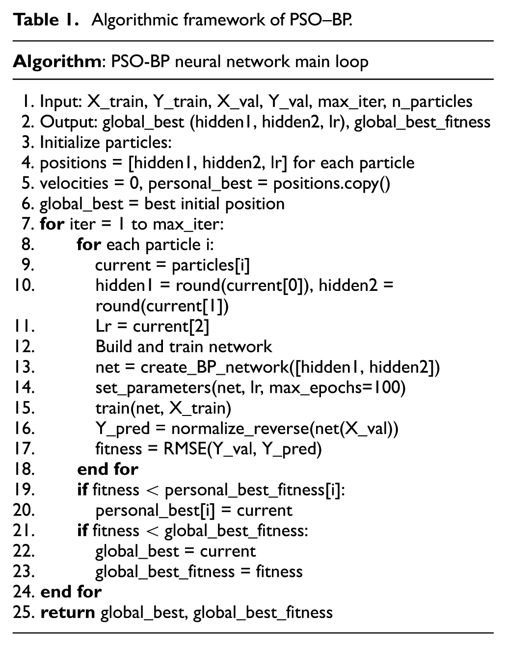
The fitness of the particle swarm is evaluated during each iteration, with the optimization objective being to minimize the RMSE. By adjusting the velocities and positions of the particles until they meet the accuracy requirements, the optimal number of nodes in the hidden layer and the learning rate can be determined through optimization. These parameters can then be incorporated into the BP neural network for multiple training sessions, ultimately yielding the final results. The algorithmic framework of PSO–BP neural network main loop is shown in Table 1 below.

Table 1.

Algorithmic framework of PSO–BP.

Algorithm: PSO-BP neural network main loop
1. Input: X_train, Y_train, X_val, Y_val, max_iter, n_particles 2. Output: global_best (hidden1, hidden2, lr), global_best_fitness 3. Initialize particles: 4. positions = [hidden1, hidden2, lr] for each particle 5. velocities = 0, personal_best = positions.copy() 6. global_best = best initial position 7. for iter = 1 to max_iter: 8. for each particle i: 9. current = particles[i] 10. hidden1 = round(current[0]), hidden2 = round(current[1]) 11. Lr = current[2] 12. Build and train network 13. net = create_BP_network([hidden1, hidden2]) 14. set_parameters(net, lr, max_epochs=100) 15. train(net, X_train) 16. Y_pred = normalize_reverse(net(X_val)) 17. fitness = RMSE(Y_val, Y_pred) 18. end for 19. if fitness < personal_best_fitness[i]: 20. personal_best[i] = current 21. if fitness < global_best_fitness: 22. global_best = current 23. global_best_fitness = fitness 24. end for 25. return global_best, global_best_fitness

Algorithm: PSO-BP neural network main loop

1. Input: X_train, Y_train, X_val, Y_val, max_iter, n_particles
2. Output: global_best (hidden1, hidden2, lr), global_best_fitness
3. Initialize particles:
4. positions = [hidden1, hidden2, lr] for each particle
5. velocities = 0, personal_best = positions.copy()
6. global_best = best initial position
7. for iter = 1 to max_iter:
8. for each particle i:
9. current = particles[i]
10. hidden1 = round(current[0]), hidden2 = round(current[1])
11. Lr = current[2]
12. Build and train network
13. net = create_BP_network([hidden1, hidden2])
14. set_parameters(net, lr, max_epochs=100)
15. train(net, X_train)
16. Y_pred = normalize_reverse(net(X_val))
17. fitness = RMSE(Y_val, Y_pred)
18. end for
19. if fitness < personal_best_fitness[i]:
20. personal_best[i] = current
21. if fitness < global_best_fitness:
22. global_best = current
23. global_best_fitness = fitness
24. end for
25. return global_best, global_best_fitness

CAPSO optimization algorithm

Since the PSO–BP algorithm exhibits a pronounced phenomenon of premature convergence, it is prone to becoming trapped in local optima when addressing complex nonlinear problems.¹⁹ To mitigate this issue, chaotic initialization²⁰ is employed to generate the initial population, thereby enhancing the diversity of the population. Additionally, nonlinear inertia weights, adaptive cognitive factors, and chaotic perturbation strategies are implemented to apply chaotic perturbations to particles that have become ensnared in local optima.

This paper employs chaotic initialization by utilizing logistic mapping to generate chaotic sequences for the initialized particle population. The position of each particle is determined by iterating the logistic equation multiple times and subsequently mapping the results to the range of (−1, 1) to enhance the diversity of the initial population. By using chaotic sequences instead of random numbers to establish the initial particle positions, the population becomes more traversable, exhibits greater diversity, and is better equipped to overcome the challenges posed by local optima. This approach contributes to the superior performance of the algorithm. The logistic equation used for generating the initial population in this study is shown in equation (11).

z_{n + 1} = μ z_{n} (1 - z_{n})

(11)

In equation (11), $z_{n}$ is chaotic variable, $μ$ is chaos parameter, it generates pseudo-random sequences with ergodicity and initial value sensitivity. It is taken as 4 in this study.

The inertia weight w²¹ determines the extent to which the current velocity is influenced by previous velocities. Its value significantly impacts both the accuracy of the algorithm and the speed of convergence. In the early stages of iteration, utilizing a larger w enhances the particles’ velocity and global search capability. Conversely, in the later stages of iteration, employing a smaller weight reduces the particles’ velocity, allowing them to concentrate on local search, thereby improving the accuracy of the optimal solution. As the iteration progresses, the inertia weights decrease linearly. In this paper, we implement dynamic inertia weights to adaptively adjust the local and global search capabilities of the particles. The adjustment strategy during iteration is shown in equation (12).

w = w_{\max} - (w_{\max} - w_{\min}) \times \frac{t}{T}

(12)

In equation (12), $t$ is the current iteration, $T$ is the total number of iterations, $w_{\max}$ and $w_{\min}$ are the largest and smallest values of the inertia weights, respectively.

This algorithm incorporates cognitive adaptive learning factors²² $c_{1}$ and $c_{2}$ to enable rapid exploration of the entire search space in the early stages, while also enhancing the accuracy and convergence speed in the later stages. The learning factors can be adjusted according to the search state to balance individual experience with group collaboration. In most existing studies, these factors are typically treated as constants, and in this paper, they will be set to 2 for both parameters.

After each iteration, chaotic perturbations are continuously applied to the global optimal position. A chaotic sequence is generated and added to the position of $g_{best}$ ,²³ which is then constrained to the range of (−1, 1). This approach enables the particles to explore the normalized parameter space from start to finish. Chaotic perturbations enhance the ability to escape local optima, preventing the algorithm from becoming trapped in premature convergence and improving the global search capability. The equation for the chaotic perturbation is shown in equation (13).

gbes t_{n} = gbes t_{n - 1} + η \times chao s_{sequency}

(13)

In equation (13), $η$ is the disturbance intensity, this paper takes it as 1. It helps jump out of local optimality by introducing chaotic noise.

When the algorithm experiences premature convergence, the position variables are updated according to equation (14):

x_{t + 1} = x_{\min} + z_{i + 1} \times (x_{\max} - x_{\min})

(14)

In equation (14), $z_{n}$ is chaotic variable, which is the same as above.

In the main loop of the CAPSO algorithm, the velocities and positions of the particles are updated at each iteration according to the principles of the PSO algorithm. RMSE is used as the fitness value for each particle. Once the fitness value converges to the optimal solution, the CAPSO optimization process is complete, and the optimal solution is utilized as a parameter for training the BP neural network. The algorithmic framework of CAPSO–BP is shown in Table 2. After predicting the data of testing set, the RMSE, MSE, and correlation coefficient (R) of the training results are compared. The equations for calculating RMSE and MSE are shown in equations (15) to (17):

RMSE = \sqrt{\frac{1}{n} \sum_{i = 1}^{n} {(y_{i} - {\hat{y}}_{i})}^{2}}

(15)

MSE = \frac{1}{n} \sum_{i = 1}^{n} (y_{i} - {\hat{y}}_{i})^{2}

(16)

R = \frac{Cov (x, y)}{\sqrt{Var [x] Var [y]}}

(17)

Table 2.

Algorithmic framework of CAPSO–BP.

Algorithm: CAPSO-BP neural network main loop
1. Input: X_train, Y_train, T(max_iters), N(particles) 2. Output: gbest_position, gbest_score 3. Initialize: 4. positions[N,D] ∈ [-1,1], velocities[N,D] = 0 5. pbest = positions, gbest = best initial 6. Set w_max, w_min, c1, c2, μ=4 7. for iter = 1 to T: 8. w = w_max - (w_max - w_min)×iter/T 9. for each particle i: 10. Update velocity:v[i]=w×v[i]+c1×rand()×(pbest[i]-pos[i])+c2×rand()×(gbest- pos[i]) 11. Update position: pos[i] = clamp(pos[i] + v[i], [-1,1]) 12. net = BP_network(pos[i]) # Set weights 13. rmse = RMSE(net(X_train), Y_train) 14. if rmse < pbest[i].score: 15. pbest[i] = pos[i], pbest[i].score = rmse 16. if rmse < gbest.score: 17. gbest = pos[i], gbest.score = rmse 18. end for 19. chaos = 2×Logistic_map(μ, D) - 1 # μ=4, scale to [-1,1] 20. gbest = clamp(gbest + 0.1×chaos, [-1,1]) 22. print(f"Iter {iter}, Best RMSE: {gbest.score:.4f}") 22. end for 23. return gbest

Algorithm: CAPSO-BP neural network main loop

1. Input: X_train, Y_train, T(max_iters), N(particles)
2. Output: gbest_position, gbest_score
3. Initialize:
4. positions[N,D] ∈ [-1,1], velocities[N,D] = 0
5. pbest = positions, gbest = best initial
6. Set w_max, w_min, c1, c2, μ=4
7. for iter = 1 to T:
8. w = w_max - (w_max - w_min)×iter/T
9. for each particle i:
10. Update velocity:v[i]=w×v[i]+c1×rand()×(pbest[i]-pos[i])+c2×rand()×(gbest- pos[i])
11. Update position: pos[i] = clamp(pos[i] + v[i], [-1,1])
12. net = BP_network(pos[i]) # Set weights
13. rmse = RMSE(net(X_train), Y_train)
14. if rmse < pbest[i].score:
15. pbest[i] = pos[i], pbest[i].score = rmse
16. if rmse < gbest.score:
17. gbest = pos[i], gbest.score = rmse
18. end for
19. chaos = 2×Logistic_map(μ, D) - 1 # μ=4, scale to [-1,1]
20. gbest = clamp(gbest + 0.1×chaos, [-1,1])
22. print(f"Iter {iter}, Best RMSE: {gbest.score:.4f}")
22. end for
23. return gbest

In equation (17), $x, y$ are two variables, $Cov (x, y)$ is the covariance of $x$ and $y$ , $Var [x]$ is the variance of $x$ , $Var [y]$ is the variance of $y$ .

The general flowchart of the optimization algorithm in this paper is shown in Figure 1.

Figure 1.

Flowchart of the optimization algorithm.

Experiment

Preprocessing

This model predicts the peak traffic flow during weekday evenings at the intersection of Feicui Road and Danxia Road in Hefei City, Anhui Province, China. A map of this road section is presented in Figure 2. Data were collected manually at 5-min intervals from 5:30 p.m. to 6:30 p.m. between June 3 and July 15, 2024. A screenshot of the data collection process is also shown in Figure 2. A total of 300 data sets were gathered, with each set recorded simultaneously by five different volunteers during the same time interval. These data sets were verified for consistency before being utilized in this paper, ensuring their accuracy. Vehicles were classified into categories: car, heavy truck, medium truck, bus, and taxi. The results from 25 days of data collection, including traffic flow and vehicle types, are illustrated in Figure 3. In order to avoid affecting the effectiveness of the solution algorithm and to facilitate the training of the neural network, the data are normalized to the range of (0, 1). The preprocessing operation helps to enhance the correlation of the data, making the data more suitable for subsequent analysis. It also improves the convergence speed of the algorithm and speeds up the calculation process. Through preprocessing, the consistency and reliability of the traffic flow data are ensured and the noise effect is attenuated. Such processing makes the data more suitable for subsequent analysis and modeling, improving the consistency and reliability of the data.

Figure 2.

The screenshot of the data collection.

Figure 3.

3D map of aggregated traffic flow data classification.

Next, the collected 300 data sets are divided into a training set and a testing set. Based on the temporal characteristics of the data, the data are organized in a time series format.²⁴ Using the traffic flow data from three consecutive time points as input, and the predicted traffic flow value at the next time point as output, this paper establishes the length of the time window as 3, allocating 70% of the total dataset for the training set and the remaining 30% for the testing set.

In the process of configuring the parameters of the neural network, there are two hidden layers. The first hidden layer contains 10 neurons, while the second layer consists of five neurons. The training algorithm employed is the Levenberg-Marquardt method, the error measurement is based on MSE and the compilation algorithm utilizes MEX.

Training results

To better demonstrate the training results, this paper introduces linear regression plots and error distribution histograms to visually represent prediction accuracy.²⁵ The linear regression plot displays the relationship between actual values and predicted values through a scatter diagram, which can intuitively reveal whether the model exhibits systematic bias. The error distribution histogram, on the other hand, analyzes model performance from a different perspective by showing the distribution characteristics of prediction errors. The skewness of the distribution reflects the asymmetry of errors, while the width of the distribution indicates the precision of the model.²⁶

The results of training using a traditional BP neural network are presented below. Figure 4 illustrates the data regression for the training and testing sets, respectively. This paper conducts a linear regression analysis of the target values in relation to the neural network outputs. The R value for the training set is 0.99948, indicating that the neural network model performs well on the known data of the training set. In contrast, the R value for the testing set is 0.90602, suggesting that the linear regression performance on the testing set is inferior compared to that of the training set. Consequently, the model exhibits a significant error when predicting unknown data. Figure 5 illustrates the histograms of the error distribution for the prediction data across both the training and testing sets. The errors in the training set are predominantly clustered near the zero line, aligning with the expectations of linear regression. In contrast, the testing set exhibits some deviation from this trend. Considering the characteristics of the BP neural network, the most likely cause of these errors is the model’s convergence to a local optimum during the training iterations, which results in a premature termination of the search for the extremes of the loss function. The Mu value of this neural network model is only 1e-10, reaching the lowest threshold set, indicating issues with inconspicuous and poor data convergence. Furthermore, the BP neural network operates with a low learning rate during training, which leads to slow data updates, reduced training efficiency, and extended training times, all of which hinder the model’s development. Finally, 210 data sets from the training set and 90 data sets from the testing set will be presented in two figures within a window to compare the predicted results with the actual values, as depicted in Figure 6. It is important to note that the training results obtained from each iteration of the BP neural network exhibit slight variations. This variability arises because the neural network may converge to different local optima during training.

Figure 4.

Linear regression of BP neural network training and testing set.

Figure 5.

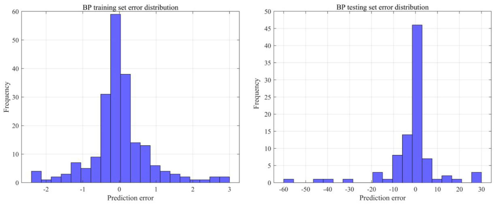
Histogram of error distribution in the training and testing set of BP neural network.

Figure 6.

Comparison of BP neural network prediction results.(Content circled in red shows the testing set data comparison)

This paper introduces the PSO algorithm to optimize the hidden layer node count and learning rate of BP neural network. The hidden layer node count and learning rate are incorporated into the position of each particle. For each particle, a combination of the number of hidden layer nodes and the learning rate is created, allowing us to construct the BP network. We then set the training parameters and train the network using the training set, after which the error is computed on the training set to determine the fitness value. The optimal values are selected through particle swarm comparison and subsequently integrated into the neural network for training, resulting in the final prediction. After 30 iterations, the optimal fitness value is 1.6847, and the optimal configuration consists of two hidden layers: the first layer contains five neurons, while the second layer contains three neurons. Figure 7 illustrates the regression plots for the training and testing datasets. The R value for the training set is 0.998, and for the testing set, it is 0.936. Compared to the BP neural network model, the R value for the testing set increases by 3.33%. This indicates that the predicted values exhibit a significantly stronger linear correlation with the true values than those produced by the traditional BP neural network, aligning with the optimization objective. Figure 8 presents the error distribution histograms. The PSO–BP neural network errors are predominantly clustered near the zero line, with a higher density compared to the BP neural network, suggesting a significant optimization effect. Figure 9 displays a side-by-side comparison of the true values and predicted values for the 210 training sets and 90 testing sets. This optimized network still has a tendency to fall into local optimal solutions

Figure 7.

Linear regression of PSO–BP neural network training and testing set.

Figure 8.

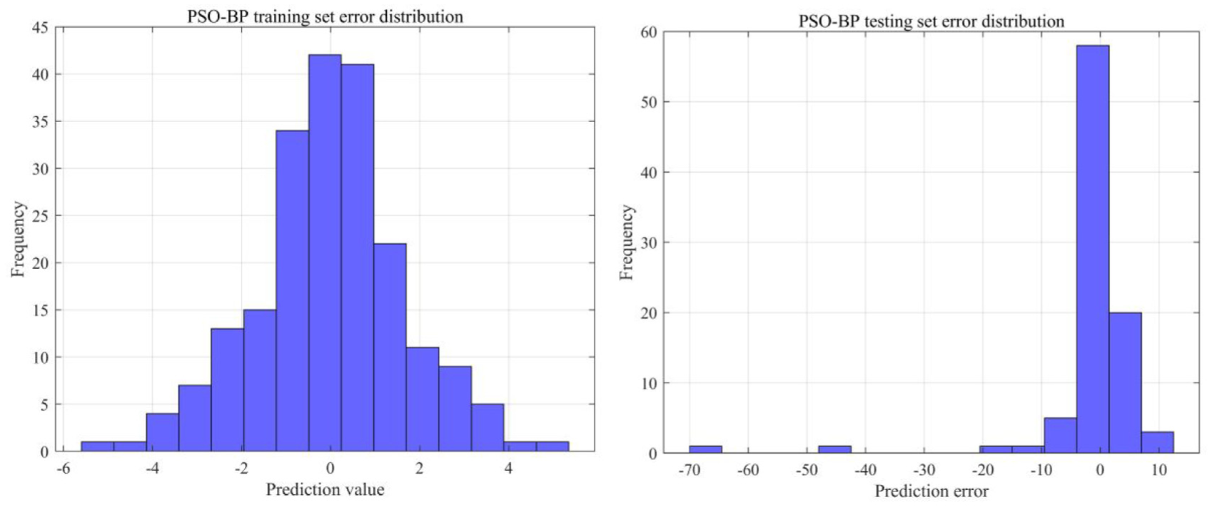
Histogram of error distribution in the training and testing set of PSO–BP neural network.

Figure 9.

Comparison of PSO–BP neural network prediction results.(Content circled in red shows the testing set data comparison).

The adaptive chaos algorithm is applied to PSO–BP algorithm for optimization. Following particle initialization, this paper implements chaos mapping, non-linear weights, and cognitive adaptive factors. After conducting iterative optimization, this paper incorporates the optimal solution into the BP neural network for propagation, and the prediction results after training are as follows. After 50 iterations, the optimal fitness value achieved is 0.3012. As illustrated in Figure 10, this paper analyzes the linear regression between the actual values and the predicted values for both the training and testing sets. The R for the training set is 0.99747, while it is 0.98962 for the testing set. The linear fit demonstrates an improvement of 9.23% compared to BP neural network and an enhancement of 5.70% compared to the PSO–BP. The histograms depicting the error distribution for the CAPSO–BP training and testing sets are presented in Figure 11. The errors are notably more concentrated around the zero line, indicating superior model prediction results, which is further validated in Figure 12, showcasing the comparison of CAPSO–BP neural network prediction outcomes. Through optimization, the CAPSO–BP network no longer suffers from falling into local optimal solutions, as observed in the two networks mentioned above. The results obtained from multiple training sessions are consistent.

Figure 10.

Linear regression of CAPSO–BP neural network training and training set.

Figure 11.

Histogram of error distribution in the training and testing set of CAPSO–BP neural network.

Figure 12.

Comparison of CAPSO–BP neural network prediction results.(Content circled in red shows the testing set data comparison).

Finally, this paper consistently controls the relevant setup parameters and compares the prediction results of the BP neural network, PSO–BP neural network, CAPSO–BP neural network, LSTM model, and GNN model across the samples. As shown in Table 3, the three algorithms discussed in this paper are compared with those referenced in terms of relevant parameter indicators. The results indicate that the MSE of the BP neural network decreases significantly after optimization by CAPSO. This optimization results in the highest prediction accuracy, strengthens the linear correlation of the data, and achieves the best fitting effect, aligning with the research expectations outlined in this paper.

Table 3.

Several neural network algorithms relevant metrics.

Methods	Training set RMSE	Testing set RMSE	Training set MSE	Testing set MSE	Training set R	Testing set R
BP	0.8173	11.7867	0.6679	138.9268	0.9995	0.9060
PSO–BP	1.6563	9.2078	2.7434	84.7830	0.9979	0.9362
CAPSO–BP	1.8126	3.7057	3.2854	13.7325	0.9975	0.9896
GNN²⁷	–	–	–	–	–	0.979
LSTM²⁷	–	–	–	–	–	0.980

Based on the analysis of the above results, the following conclusions can be drawn:

CAPSO–BP algorithm offers significant advantages in prediction accuracy, as evidenced by a substantial reduction in the MSE value is greatly reduced compared to traditional BP neural networks and PSO–BP. This improvement is largely attributed to the adaptive adjustment of the particle swarm and the implementation of a chaotic perturbation strategy, which greatly enhances the particles’ ability to locate the optimal solution while avoiding convergence to local optima.

In terms of linear regression, the R value of the CAPSO–BP testing set increases by 9.23% compared to that of the traditional BP neural network, and by 5.70% compared to that of PSO–BP. This indicates that CAPSO–BP demonstrates superior linear regression performance and confirms its enhanced prediction accuracy.

Compared to other neural network models discussed in the literature, the improved PSO–BP neural network demonstrates higher accuracy in predicting short-term traffic flow at urban road intersections, despite differences in parameter and variable settings from the algorithms used in this study.

Through the optimization of the CAPSO algorithm, the training results are no longer confined to local optimal solutions, as is the case with the BP and PSO algorithms. This enhancement ensures both the accuracy and stability of the results.

Conclusions

According to the task of short-term traffic flow prediction at urban road intersections, this study focuses on traffic flows during the evening rush hour at the planar intersection of Feicui Road and Danxia Road in Hefei City, Anhui Province, China. Data were collected at the same time every day for 25 consecutive working days. Each inlet was recorded by five volunteers at 5-min intervals for a total duration of 1 h, and the collected data was verified to ensure its accuracy.

This study compares the traditional BP neural network model, the PSO–BP neural network model, and the CAPSO–BP neural network model to predict traffic flow at intersections. The results demonstrate the advantages of the CAPSO–BP model in forecasting short-term traffic flow at urban road intersections. This research not only enhances theoretical knowledge with empirical analyses of case studies but also offers a decision-making foundation for traffic control. Furthermore, it establishes a new basis for the development of smart cities, which holds significant practical and research implications.

However, this study has the following limitations.

This study only predicts weekday evening peaks at one intersection, ignoring weather, holidays, and surrounding traffic. Although vehicle types were recorded, their different road occupancy and driving behaviors weren’t fully modeled. Traffic from all directions was merged, losing directional details. These simplifications hurt practical accuracy.

CAPSO–BP improves global search but is computationally expensive. Tuning its many hyperparameters is complex. The method may overfit small datasets, hurting generalization.

The model predicts total intersection flow, not directional counts needed for signal control or tidal lanes. Its focus on one site and time reduces generalizability. Future work needs richer data, vehicle and direction-specific models, and more robust algorithms.

In future research, the existing prediction model could be enhanced by quantifying spatiotemporal features and other environmental influencing factors, introducing a traffic flow prediction model that incorporates vehicle-type weighting, and conducting directional traffic flow studies. These improvements would provide more accurate data support for intersection signal timing optimization and traffic organization design.

Footnotes

Handling Editor: Divyam Semwal

ORCID iD

Chengqun Qiu

Funding

The authors disclosed receipt of the following financial support for the research, authorship, and/or publication of this article: This study was supported by the National Natural Science Foundation of China (no. 52002156) and the Jiangsu Natural Science Foundation of China (no. BK20211364).

Declaration of conflicting interests

The authors declared no potential conflicts of interest with respect to the research, authorship, and/or publication of this article.

References

Hussain

Afzal

Ahmad

, et al. Intelligent traffic flow prediction using optimized GRU model. IEEE Access 2021; 9: 100736–100746.

Polson

Sokolov

VO.

Deep learning for short-term traffic flow prediction. Transp Res C Emerg Technol 2017; 79: 1–17.

Huang

Chen

Sun

, et al. Short-term traffic prediction based on time series decomposition. Phys A Stat Mech Appl 2022; 585: 126441.

Song

Duan

Cheng

A novel fractional-order grey Euler prediction model and its application in short-term traffic flow. Chaos Solitons Fractals 2024; 189: 115722.

Zaraket

Harb

Bennis

, et al. Hyper-Flophet: a neural prophet-based model for traffic flow forecasting in transportation systems. Simul Model Pract Theory 2024; 134: 102954.

Research on traffic flow prediction method based on adaptive multi-channel graph convolutional neural networks. Adv Eng Innov 2024; 7: 41–47.

Lieskovska

Jakubec

Kudela

Traffic flow prediction in urban networks: integrating sequential neural network architectures. Int J Adv Comput Sci Appl 2024; 15: 708–714.

Liu

Zhang

An adaptive traffic flow prediction model based on spatiotemporal graph neural network. J Supercomput 2023; 79: 15245–15269.

Zhao

Guo

Dai

, et al. Multi-step trend aware graph neural network for traffic flow forecasting. Big Data Res 2024; 38: 100482.

10.

Mrad

Mraihi

Murthy

AS.

Efficient implementation of a wavelet neural network model for short-term traffic flow prediction: sensitivity analysis. Int J Transp Sci Technol 2024; 17: 21–38.

11.

Jiang

Yin

Wei

, et al. Industrial carbon emission efficiency prediction and carbon emission reduction strategies based on multi-objective particle swarm optimization-backpropagation: a perspective from regional clustering. Sci Total Environ 2024; 906: 167692.

12.

Yang

Qiang

, et al. A network traffic forecasting method based on SA optimized ARIMA–BP neural network. Comput Netw 2021; 193: 108102.

13.

Hong

, et al. Short term electric load forecasting model and its verification for process industrial enterprises based on hybrid GA–PSO–BPNN algorithm—a case study of papermaking process. Energy 2019; 170: 1215–1227.

14.

Omar

Yakub

Abdullah

, et al. One-step vs horizon-step training strategies for multi-step traffic flow forecasting with direct particle swarm optimization grid search support vector regression and long short-term memory. Expert Syst Appl 2024; 252: 124154.

15.

Hong

Kang

Urban traffic flow forecasting using Gauss–SVR with cat mapping, cloud model and PSO hybrid algorithm. Neurocomputing 2013; 99: 230–240.

16.

Bharti Redhu

Kumar

Short-term traffic flow prediction based on optimized deep learning neural network: PSO-Bi-LSTM. Phys A Stat Mech Appl 2023; 625: 129001.

17.

Xiao

Luo

Chen

, et al. Prediction model of asphalt pavement functional and structural performance using PSO–BPNN algorithm. Constr Build Mater 2023; 407: 133534.

18.

Chen

Liu

, et al. Air pollution prediction based on optimized deep learning neural networks: PSO–LSTM. Atmos Pollut Res 2025; 16: 102413.

19.

Beheshti

Hj Shamsuddin

SM.

CAPSO: centripetal accelerated particle swarm optimization. Inf Sci 2014; 258: 54–79.

20.

Yan

Zhang

, et al. Short-term traffic flow prediction based on a hybrid optimization algorithm. Appl Math Model 2022; 102: 385–404.

21.

Duan

Chen

Chang

, et al. CAPSO: chaos adaptive particle swarm optimization algorithm. IEEE Access 2022; 10: 29393–29405.

22.

Jose

Vigila

SMC

. F-CAPSO: fuzzy chaos adaptive particle swarm optimization for energy-efficient and secure data transmission in MANET. Expert Syst Appl 2023; 234: 120944.

23.

Taghavifar

Rakheja

Reina

A novel optimal path-planning and following algorithm for wheeled robots on deformable terrains. J Terramech 2021; 96: 147–157.

24.

Hou

Leng

, et al. An adaptive hybrid model for short-term urban traffic flow prediction. Phys A Stat Mech Appl 2019; 527: 121065.

25.

Hasan

Alsubaie

MSA

, et al. Diagnosis of tobacco addiction using medical signal: an EEG-based time-frequency domain analysis using machine learning. Adv Sci Technol Eng Syst J 2021; 6(1): 842–849.

26.

Hasan Shahariar

Bodisco

Surawski

, et al. Real-driving CO₂, NO_x and fuel consumption estimation using machine learning approaches. Next Energy 2023; 1(4): 100060.

27.

Cao

Chang

Chen

A comparative study of traffic flow prediction methods based on neural networks. Sci Technol Innov 2024; 13: 42–44.

Optimization of BP neural network traffic flow prediction model based on improved particle swarm algorithm

Abstract

Keywords

Introduction

Methods

BP neural network

PSO–BP optimization algorithm

CAPSO optimization algorithm

Experiment

Preprocessing

Training results

Conclusions

Footnotes

ORCID iD

Funding

Declaration of conflicting interests

References