
Abstract
The reliability analysis of railway rolling stock systems determines how efficiently passenger services operate and how sustainable operations remain over a specified period. The proposed framework presented in this paper implements supervised learning to predict system downtime while using time-series forecasting to evaluate incident risk levels. Three regression models, Bayesian Ridge Regression, Support Vector Regression (SVR), and K-Nearest Neighbors (KNN), were trained on historical failure records to estimate Mean Time to Repair (MTTR). The naive baseline MTTR data is used as input for modelling and prediction downtimes, and further analysis using the Bayesian Ridge model provided the most accurate results. Seasonal Autoregressive Integrated Moving Average with Exogenous variables (SARIMAX), Long Short-Term Memory networks, Convolutional Neural Networks, and Exponential Smoothing approaches were used to analyse weekly and monthly CCTV camera failure incidents. The risk of system failure incidents was classified as low, medium, and high-risk levels to support decisions on maintenance schedules, spare parts, and resource allocation in advance. The dynamic modelling using machine learning and time series modelling approach presented in this paper can support maintenance managers make decision on optimal preventive maintenance activities and hence reduce maintenance downtimes.
Introduction
The performance of rolling stock and the condition of rail infrastructure are tightly interlinked: poor train reliability increases track occupancy and congestion, while degraded infrastructure (track geometry or signalling failures) accelerates wheel-rail wear and leads to more frequent train breakdowns. For example, Network Rail’s 2019 infrastructure report indicates that a 1% increase in rolling stock unavailability results in a 0.5% increase in annual minutes of delays across the network. 1 Similarly, the UIC’s 2020 global rail performance report indicates that infrastructure defects are responsible for up to 30% of all rolling stock failures globally. 2 Therefore, it is essential to optimise both elements in tandem to reduce delays, cancellations and life-cycle costs. Table 1 shows that between 2020 and November 2024, the CCTV systems contributed to 28.9% of the technical incidents recorded, the largest number of technical incidents, which exceeds all other systems. The Passenger Bodyside Doors, together with the Passenger Information System (PIS), have the second-highest number of reported incidents, at 11.8% each. The high frequency of CCTV system incidents requires maintenance intervention because they directly affect system reliability and service operations. The CCTV system represents the most common and disruptive technical issues which lead to most of the operational delays, cancellations, and reduction in overall performance effectiveness. 3 The research investigation presented in this paper evaluate CCTV system failure patterns to reduce the impact on service operations.
Top 10 system technical incidents (January 2020–November 2024).

In this paper trend analysis of historical CCTV failure data is conducted using forecasting and machine learning model to, predict downtime (Mean Time to Repair – MTTR) and predicting the likelihood of incidents occurring at different locations. The Support Vector Regression (SVR), Bayesian Ridge Regression, and K-Nearest Neighbors (KNN) are the three machine learning methods utilised for downtime prediction. These models are selected to analyse the CCTV system failure records because they can handle complex data configuration and provide reliable predictions. A probabilistic method for making predictions that accounts for uncertainty is presented by Tipping 4 using the Bayesian Ridge Regression model. The SVR model can convert input data into a higher-dimensional feature space and is widely recognised for its effectiveness in non-linear regression. 5 KNN predicts downtime by first locating the k-nearest neighbors of a data point and then calculating their average downtime. 6 The forecasting of location-specific incidents utilises various time series forecasting models to determine which locations are likely to experience more CCTV failures. The forecasting models considered include SARIMAX, LSTM, CNN, and ETS, respectively. 7 Seasonality and trends in the event data are handled using the SARIMAX model (Seasonal AutoRegressive Integrated Moving Average with eXogenous regressors). 8 The LSTM network is used because it can recognise connections over a distance. 9 The CNN (Convolutional Neural Network) model is commonly employed in image processing and is modified for time series forecasting. It has the ability and capacity to identify local patterns in the data. 10 Finally, ETS (Exponential Smoothing State Space Models) is used to capture both trend and seasonality in the time series data for incident forecasting. 11 The analysis of CCTV failure dynamics using these machine learning and forecasting methods enables more accurate prediction of future incidents, leading to more efficient proactive maintenance strategies. The analysis conducted and results presented in this paper identify which locations face the highest risk of CCTV failure, allowing for informed maintenance decisions and the allocation of resources to minimise downtime and improve overall fleet performance.
Literature review
The railway industry has embraced the predictive maintenance (PDM) approach as part of the Industry 4.0 paradigm, utilising IoT sensors and big data analytics. Data-driven PDM for railways is advancing toward deep learning, unsupervised anomaly detection, and ensemble methods. 12 De Simone et al. 13 developed an LSTM-based deep learning model that predicts critical failures in railway rolling stock equipment and demonstrates how modern AI can reduce train unavailability. Meira et al. 14 created a framework based on data for a train’s air production unit (APU), which combined streaming anomaly detection with one-class KNN to identify early signs of failure. The SVR model has been widely used in predictive maintenance studies as a baseline and often as a top performer on smaller datasets. In the railway domain, SVR is frequently listed among the “popular” regression techniques for RUL prediction and equipment failure forecasting. 12 Das Chagas Moura et al. 15 focus on failure time prediction for complex systems, combining signal processing with SVR to predict the time to failure in railway point machines. They note that SVR can capture the non-linear degradation trend and outperform simple linear regression. Meira et al. 14 developed an unsupervised anomaly detection framework for a train’s air production unit (APU) that uses a Half-Space Trees algorithm with a One-Class KNN to detect outliers in real-time. Kaewunruen et al. 16 employed a Bayesian Ridge Regression model to predict properties in railway infrastructure design, finding it to perform as well as, or better than, more complex nonlinear models. According to Sun et al., 17 when it comes to handling real-world unpredictability and high similarity conditions across different operational states, compared to other classifiers such as 1-Nearest Neighbor (1NN), Random Forest (RF), and Naive Bayes (NB), the Support Vector Machine (SVM) with a radial basis function kernel outperforms them. Machine learning algorithms, including logistic regression, random forest, decision trees, and k-nearest neighbor, were used by Asha and Gupta. 18 These models are used to determine the likelihood of a train being delayed based on real-time data analysis. Elahi et al. 19 (2023) identified 42 articles from January 2017 to May 2023 to examine current trends and well-known AI methods, including Support Vector Machines (SVM), Bayesian Networks, Generative Adversarial Networks (GAN), and Convolutional Neural Networks (CNN). Varshavskiy et al. 20 employed forecasting methods, including LSTM (Long Short-Term Memory) networks, in addition to traditional time series models such as ARIMA and SARIMA. These models were used to forecast ticket demand using search queries and historical data. A hybrid model that incorporates SARIMA is proposed by Chen et al. 21 and LSTM neural networks. This model is proposed to leverage the advantages of both conventional statistical approaches and contemporary machine learning methods for enhanced forecasting. The SARIMA (p, d, q) (P, D, Q) model represents the SARIMA model, where the parameters represent different features of the model, including autoregressive and moving average components for both the seasonal and non-seasonal parts of the time series. According to Astuti, 22 the SARIMA model is an extension of the ARIMA model that includes seasonal patterns in time series data.
Data collection and analysis
The analysis presented in this paper uses two forms of datasets collected from January 2020 to November 2024, focusing on CCTV-related technical failures:
The CCTV system data set used for analysis are from two different integrated databases (CORMAP and the Central Control System database (CCS)). The CCS database records a broader range of data information, which includes all technical anomalies detected by the train’s onboard expert system, and the CORMAP database is linked to the CCS database. The 109 CCTV-related cases presented in Table 1 were manually extracted from the CORMAP database system, which logs only confirmed technical failures that result in delays, partial, or full-service cancellations across multiple subsystems. The CCTV system was identified as the most frequently reported failure type affecting the fleet service operation and was selected for downtime prediction analysis. The 1454 CCTV fault entries, which also include the 109 technical failures, signals, and failures, come from the Central Control Unit (CCU). The CCU captures a broader range of data sets, and we consider using it for forecasting fault trends and identifying high-risk locations where these incidents occur. Both datasets were collected automatically daily, using the operator’s standardised digital fault-logging infrastructure. Each entry includes structured attributes such as INCIDENT_DATE, STATUS_DATE, train or unit ID, subsystem, fault summary, and classification levels (Primary, Secondary, Tertiary). Missing data were handled based on impact: entries missing non-critical fields such as cab ID, secondary and tertiary classification, missing location from GPS were retained, while entries missing key attributes (timestamp or fault type) were excluded to preserve model integrity. The original CCTV failure incident data is split into weekly and monthly format as depicted in the time series data graph in Figure 1.

Plot of weekly and monthly time series data of CCTV failure incidents.
The UK railway operates on a standard reporting calendar which spans from April to March, with 13 operational periods of 28 days each. This structure ensures full seasonal and annual coverage. The dataset contains continuous operation events of fleet periods, which captures a fair distribution of technical faults across operational lifespans.
Figure 2 shows data that includes the number of CCTV system failures per week, along with its long-term pattern, weekly patterns, and random variations. The trend shows a flat pattern of 4–5 incidents per week from early 2020 through mid-2022 before it rises gradually to about 9–10 incidents per week in late 2023, indicating a gradual rise in CCTV systems. The causes included environmental factors such as condensation or water ingress in camera pods, improper or incomplete battery reset procedures, and driver-only operator (DOO) display failures. In some cases, failures in the passenger information systems of interdependent systems also triggered or masked CCTV faults. The observed trend indicates both technical degradation and increasing system complexity over time, primarily due to operational wear accumulating across the fleet. The seasonal component shows a distinct weekly pattern because incident counts reach their highest point during the middle of the week. The residual component shows random oscillations around zero with occasional spikes that represent isolated non-seasonal events.
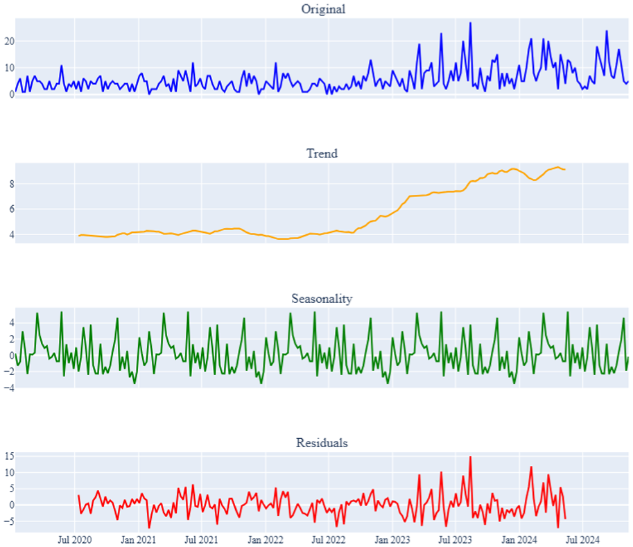
Weekly decomposed plot for CCTV failure incidents.
Figure 3 original series shows the incident counts per month; there is a gradual rise in failure incidents after mid-2022 and a pronounced spike in late 2023. Trend data indicate a smoothed, long-term increase from approximately 15 failures per month in early 2020 to nearly 40 incidents per month by mid-2024, reflecting progressive wear, ageing equipment, and changes in operational intensity. The seasonal component exhibits a clear 12-month cycle, with consistent failure counts. The residuals show high-frequency variability after removing trend and seasonality, therefore capturing irregular events such as maintenance backlogs. The trend component in both series shows an apparent upward drift, with weekly failures increasing from about 1–2 incidents in 2020 to 8–10 by the end of 2024, and monthly counts from about 15 to about 40 over the same period, indicating strong non-stationarity and motivating first-order differencing (d = 1, D = 1) in our SARIMAX and ETS models. The low-magnitude residuals indicate that there is little autocorrelated structure remaining after removing trend and seasonality, suggesting that our chosen SARIMAX and smoothing components are sufficient without additional exogenous inputs. By matching differencing and seasonal hyperparameters to these decomposition results, we can be confident that each forecasting model will accurately capture both the long-term growth and the strong annual rhythm, thus enabling maintenance planners to schedule activities appropriately.
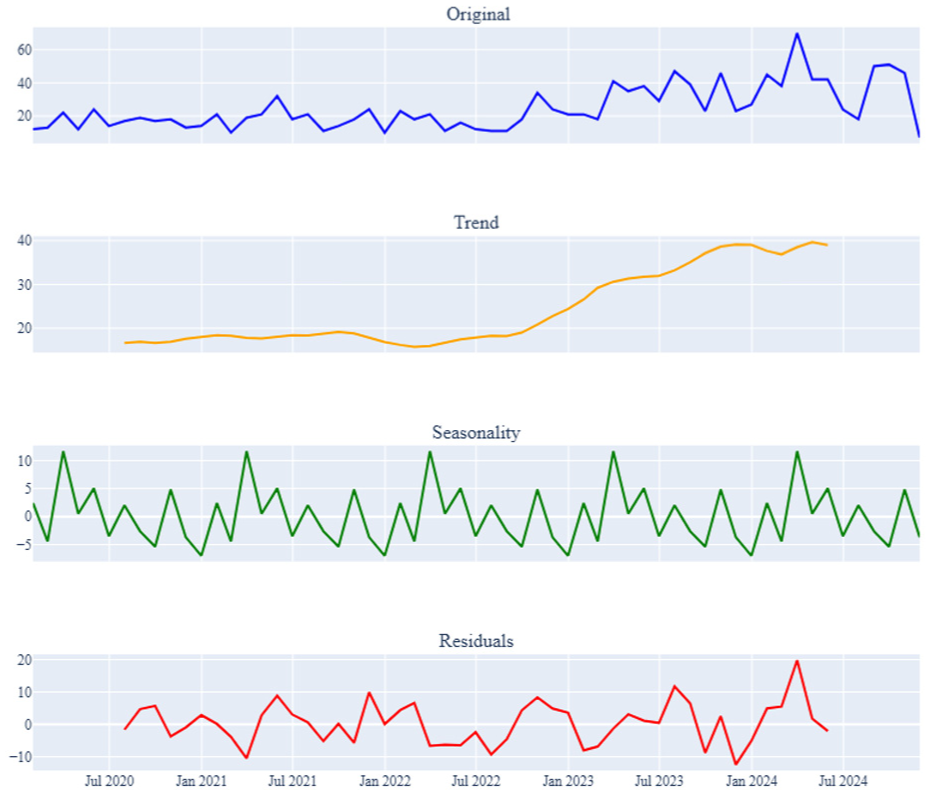
Monthly decomposed plot for CCTV failure incidents.
Methodology
This paper presents two separate predictive models developed to enhance the maintenance operations of CCTV systems for Class 380 Electric Multiple Unit train. The fleet consists of 22 three-car units and 16 four-car units. A total of 38 units, which operate on electrified routes in Scotland. The EMUs that run on electrified Scottish routes have a uniform onboard CCTV system which maintains consistent data throughout the entire fleet. The first layer depends on supervised machine learning to predict downtime (MTTR), while the second layer uses time series models for incident forecasting. The dataset contains incident summaries, along with timestamps, unit data, and location details. The flow diagram in Figure 4 shows the model development process.

Flow chart of predictive and forecasting model.
Reliability metrics
We started by computing two core reliability measures representing the raw failure timestamps

Where
Predictive model
Support Vector Regression (SVR)
The SVR model applied in this research relies on the radial basis function (RBF) kernel to detect non-linear patterns in the data. The SVR decision function uses the following formula 5 :

Where,
The SVR model, utilising an RBF kernel, was employed to forecast the mean time to repair (MTTR) of the CCTV system. The dataset included both numerical and textual features. The summary fault descriptions were preprocessed through term frequency-inverse document frequency (TF-IDF) vectorisation, which selected the top 100 features to minimise dimensionality. The Standard Scaler was used to scale the numerical attributes, which included incident and status dates transformed into numeric timestamps, mean time between failures (MTBF), unit identifiers, and the reporting period.
The model combined textual and numerical features to create a single feature set. Training through a 70% train and 30% test split while using SVR parameters of kernel radial basis function = “rbf,” C (regularisation strength) = 100 and epsilon (insensitive tube width) = 0.2 to achieve proper model complexity and prediction error tolerance.
K-Nearest Neighbors (KNN)
The K-Nearest Neighbors (KNN) regression model is employed to forecast the mean time to repair (MTTR), which represents the duration of downtime when CCTV failures occur. The INCIDENT_DATE and STATUS_DATE columns are converted into numeric values using pd.to_numeric(pd.to_datetime(…)), which converts the dates into continuous numerical features. Target values of test instances are predicted by the K-Nearest Neighbors (KNN) regression model by averaging their K closest neighbors. The algorithm follows these steps:
Distance calculation: The algorithm calculates the distance

Where,
The shortest Euclidean distances determine the K closest neighbors to the test point. The predicted value
Where,
The KNN regressor implementation for MTTR prediction followed the same preprocessing steps as SVR to maintain consistency. The date fields INCIDENT_DATE and STATUS_DATE were converted into numeric timestamps. The Standard Scaler was used to standardise the numerical features, which included MTBF, unit and period, while the textual maintenance summaries were transformed using a TF-IDF vectoriser with a maximum of 100 features. The numeric and text features were combined into a single feature matrix.
The dataset was split into training and testing sets with a 70:30 ratio. A KNeighbors Regressor with k = 5 was trained on the combined feature set, meaning the model predicts downtime based on the average of the five most similar historical fault instances in the feature space. This choice of k strikes a balance between noise sensitivity (small k) and over-smoothing (large k), allowing the model to capture local patterns in both temporal and textual fault descriptors.
Regression using Bayesian ridge
Using Bayesian techniques, Bayesian ridge regression is a type of linear regression for parameter estimation, assuming that the weights are drawn from a normal prior distribution.23,24 The technique incorporates uncertainty into the predictions while determining the model parameters via maximum likelihood estimation. 25 The key distributions used in Bayesian ridge regression:
Prior Distribution for the Weights (

Where,
Likelihood function (Gaussian Likelihood for y): Given the features X and the observed data y, the likelihood function represents the weights β. It assumes that the errors (residuals) follow a normal distribution

Where,
Posterior distribution (Bayes’ theorem): The probability function and the prior distribution are combined to get the posterior distribution by Bayes’ theorem. This allows us to update our belief about the model parameters

Where,
Prediction: The distribution of

Where, X is the matrix of input features (for the test data),
Bayesian ridge regression with multimodal feature fusion
Bayesian ridge regression through a new approach, which merges structured incident data with unstructured textual maintenance reports to forecast downtime severity in EMU CCTV-related failures. Mean time to repair (MTTR) as its predictive variable because it represents actual service disruption periods instead of binary or categorical results.
The proposed methodology includes several innovative aspects. Multimodal Feature Integration uses both:
Numerical inputs: time-based incident logs (INCIDENT_DATE, STATUS_DATE), asset identifiers (UNIT, PERIOD), and reliability metrics (Mean Time Between Failures).
Unstructured text input: the SUMMARY field (free-text maintenance reports), transformed using TF-IDF vectorisation with 100 feature dimensions.
These two data types are pre-processed separately using Term Frequency-Inverse Document Frequency (TF-IDF). TF-IDF is a widely used text vectorisation technique that transforms each word or phrase into a numerical weight, reflecting how important a term is in a specific document relative to its frequency across the entire dataset. By applying TF-IDF with a dimensionality limit of 100 features, then fusing it into a single design matrix via horizontal stacking, we can achieve this. This hybrid approach allows the regression model to capture both quantitative signals and semantic patterns (“battery reset,”“condensation in pod”) associated with fault complexity. The approach offers multiple methodological benefits: uncertainty quantification serves as a critical requirement for risk-aware maintenance planning, prevents problems with multicollinearity and overfitting, and enables confidence-based decision-making. Evaluation through RMSE, MAE, and R2 metrics, while scatter plots of predicted vs actual values display results with a diagonal line representing perfect prediction. The model provides transparent results, which enable real-world deployment and interpretation.
Failure forecasting models
Stationarity check
The Augmented Dickey-Fuller (ADF) test is used to confirm stationarity when the SARIMAX model is implemented. To find out if a time series is stationary, apply the ADF test, or if its statistical properties don’t change over time. The ADF Statistic and p-value are computed. The series is regarded as stationary if the p-value is less than 0.05.

Where
We reject
SARIMAX model
CCTV failure data forecasted using Box and Jenkins 26 time series modelling technique, and weekly and monthly time series data are constructed using SARIMAX, a model for Seasonal Autoregressive Integrated Moving Average with Exogenous Variables, and its appropriateness, adaptability, and goodness of fit to our dataset. The model includes seasonality, moving average (MA) terms, and autoregressive (AR) components. The SARIMAX equation is:

Where,
The seasonal AR and MA components are included in the seasonal order, defined as (p, d, q, s). Seasonal differencing (d), Seasonal MA order (q), s = seasonal period and seasonal AR order (p). 27 This paper presents a new application which adapts to the actual operational needs of railway fault analysis. The method converts SARIMAX into a location-based risk prediction system for long-term CCTV-related fault planning across the EMU fleet.
1. Location-Based Temporal Segmentation
Individual train locations segment the dataset, and separate SARIMAX models are trained for each. This enables geographically forecasting, highlighting fault depots, routes, or junctions rather than treating the fleet as a uniform system.
2. Domain-Aligned Preprocessing and Transformation
The variance stabilisation process includes a square-root transformation for each time series, followed by augmented dickey fuller (ADF) tests to determine necessary differencing for stationarity. The seasonal parameters derive from operational frequencies (52 for weekly, 12 for monthly) to match railway maintenance cycles.
3. Forecasting with Embedded Risk Profiling
The risk assessment system uses LOW, MEDIUM, and HIGH-risk levels, which are determined by operational thresholds. The risk levels are colour-coded in visual outputs to help engineers and maintenance planners interpret the results intuitively.
4. Decision-Support for Proactive Maintenance
SARIMAX operates as a strategic planning tool. It supports:
Hotspot detection for critical locations.
The system provides risk-informed scheduling of inspection and maintenance operations and scenario projection up to 1 year ahead.
The methodology transforms SARIMAX into a domain-integrated, risk-aware planning tool, representing a new application in railway system maintenance.
Exponential Smoothing Methodology (ETS)
The Exponential Smoothing (ETS) model generates weekly and monthly incident forecasts from the CCTV failure dataset. The ETS model breaks down time series data into three fundamental elements: level, trend, and seasonality. The components are updated recursively over time using smoothing parameters.
The ETS model is expressed mathematically as:

Where,
The following recursive equations are used to update the components over time.
Level Update

Trend Update

Seasonality Update

The forecasted seasonal component:

The Exponential Smoothing (ETS) architecture was modified to predict event counts for every location at both weekly and monthly resolutions. The incident data were first aggregated to the necessary frequency before the series was temporally divided into a training set and a fixed-length holdout test set (52 steps for weekly forecasts and 12 for monthly forecasts), and missing periods were filled with zero counts. An additive ETS configuration (trend = “add,” seasonal = “add”) was fitted with seasonal periods of 52 (weekly) or 12 (monthly) via brute-force parameter optimisation to increase robustness across different data quantities. Additionally, a seasonal-naive baseline was created to guarantee forecasting accuracy. To prevent inaccurate performance interpretation, negative R2 scores were clipped to zero, and the model with the higher holdout R2 score was chosen for final reporting.
LSTM model
For CCTV incident number forecasting, the ability of Long Short-term Memory (LSTM) networks to reproduce long-term dependencies in sequential data led to their use. LSTM is a specific type of recurrent neural network (RNN) used to handle time series data and identify temporal patterns within the dataset. It can solve the vanishing gradient and the long-term relationships issue that typical RNNS have because it retains an internal state over time. The following equations define the LSTM model:
Forget Gate:

Where,
Input Gate:
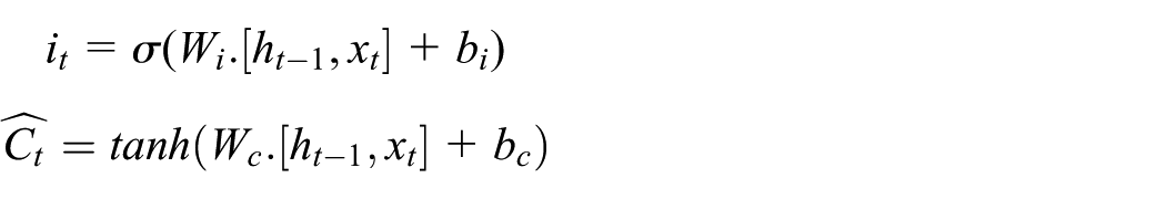
Where,
Cell state update: The contributions from the input and forget gates are combined to update the cell’s state.
Output gate: This device regulates the LSTM cell’s output.
Forecast equation:

Where
It is a compact sequence-to-one regressor network: LSTM(100, activation = ReLU) → Dropout(0.3) → Dense(50, ReLU) → Dense(1), optimised with Adam and MAE loss. The use of ReLU inside the LSTM (instead of tanh) was chosen empirically for sparse, zero-inflated differenced counts, yielding more stable gradients on our data. We enable EarlyStopping (patience = 20, best-weights restore) and ReduceLROnPlateau (factor = 0.2, patience = 10) for robust convergence. A strict chronological split (80% train, 20% test) preserves temporal causality. The model generates multi-step forecasts (52 weeks, 12 months) recursively: each new prediction is appended to the last 16 scaled steps to predict the next. Forecasts are inverse scaled, integrated back to the original level (cumulative sum plus last observed value), and then mapped to risk bands (LOW/MEDIUM/HIGH) using the operational thresholds already defined for weekly and monthly planning.
CNN model
Convolutional Neural Networks (CNN) to predict weekly and monthly incidents from the CCTV failure dataset. The ability of CNNs to detect local patterns and connections in sequential data makes them appropriate for forecasting time series. The CNN model is constructed in this manner: Using a collection of filters, 1D convolution is applied to the time series data to identify relevant patterns. The data dimensionality reduction is achieved through max-pooling, which preserves the most vital characteristics. The final forecast is created by running the retrieved information through fully connected layers.
Convolution operation: The core of the CNN is the convolution operation, which applies a filter (kernel) to a sequence of data to extract features. 29 The convolution operation represented

Where x(t) is the input time series data, w(i) is the filter (kernel) applied to the data, k is the kernel size, and * represents the convolution operation.
Max-pooling: Max-Pooling functions as a dimensionality reduction technique which maintains vital features after convolutional layers. The definition of this operation is pool(x) = max(x), where x is a window of values from the feature map or a collection of consecutive values.
Fully connected (dense) layers: Regression analysis (forecasting) is performed by running the pooled characteristics through fully connected layers. The expected event count at time t + 1 is represented by a scalar value, corresponding to the output of the CNN network. The equation for forecasting is

A 1D Convolutional Neural Network (CNN) is used to predict incident counts per location at weekly and monthly time steps. The raw counts are first-order differenced to remove trend and MinMax-scaled to [0, 1] as in the LSTM setup. A look-back window of 16 periods is used to create fixed-length temporal sequences (shape: 16 × 1) for input.
The architecture is designed to handle short noisy operational time series data:
Conv1D(128 filters, kernel size = 3, ReLU) → MaxPooling1D(pool = 2)
Conv1D(64 filters, kernel size = 2, ReLU)
Flatten → Dense (100, ReLU) → Dropout (0.3) → Dense (1 output)
The network design enables better detection of local temporal patterns, including seasonality fragments, than fully recurrent models. The pooling mechanism functions as a learned down-sampling operation. The model receives training through Adam optimisation and MAE loss functions, while Early Stopping (patience = 20) and ReduceLROnPlateau (factor = 0.2, patience = 10) prevent overfitting and automatically modify learning rates. The training-test split follows chronological order to preserve causality. The model performs recursive multi-step forecasting of 52 weeks or 12 months by incorporating each projected step into the sliding window after training. The predictions receive their risk classification as LOW, MEDIUM, or HIGH based on operational thresholds after inverse scaling and returning to the original count level.
Model evaluation
Mean Squared Error (MSE): The mean squared error is the average of the squared differences between actual and anticipated values. It is computed as:

Where,
Mean Absolute Error (MAE): The Mean Absolute Error is the average of the absolute differences between the expected and actual values. It is given by

Where,
R-squared (R2) Score: The score establishes the percentage of the variance of the dependent variable that can be accounted for by the independent variables. It is computed as
Where,
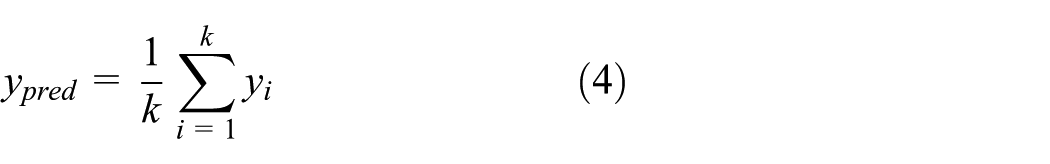
Baseline MTTR: The naïve (baseline) Mean Time To Repair equals the arithmetic mean of observed downtime values.

Where n is the number of observed incidents and
Predicted MTTR: The model’s average predicted downtime is
Percentage downtime reduction: The percentage reduction in downtime provided by the model 31 is:

Akaike Information Criterion (AIC): This is a widely used criterion for selecting models, evaluating them based on the balance between model complexity (number of parameters) and the model’s fit to the data (likelihood function). 32 The simplest model that nonetheless offers the best explanation of the data can be found with the aid of AIC.

where L is the model’s maximum likelihood and k is the number of estimated parameters.
Bayesian Information Criterion (BIC): Also known as the Schwarz Information Criterion (SIC), the BIC penalises model complexity more severely. 33 Because it penalises models with more parameters more severely than AIC, the BIC is beneficial when choosing simpler models.

Where k is the number of observations in the dataset, and the number of estimated parameters in the model is denoted by n, and the model’s maximum likelihood is L.
Risk level assignment and visualisation
To effectively interpret the forecasted values and determine the associated risk levels, we adopt a threshold-based classification for both weekly and monthly forecasts. The forecasted values
Green colour Low Risk: Incident count is below the threshold for low-risk levels.
Orange colour present Medium Risk: Incident count is within the medium risk range.
Red colour present High Risk: Incident count is above the high-risk threshold.
o Weekly: Low (<3), Medium (3–4), High (≥5).
o Monthly: Low (<10), Medium (10–19), High (≥20).
The thresholds were established based on practical operational experience and performance targets set by the railway operator for the Class 380 fleet. Weekly fault counts above five incidents are typically viewed as indicative of performance degradation, as the operator aims to maintain incident rates between 2 and 4 per week during normal operations. Similarly, monthly fault counts exceeding 20–32 incidents are generally flagged for review in maintenance and reliability assessments. As such, the Low, Medium, and High-risk levels are aligned with real-world expectations and routine maintenance planning protocols.
Results and analysis
Prediction-performance and downtime impact
Three regression algorithms, including Support Vector Regression (SVR), 5 K-Nearest Neighbors (KNN), 6 and Bayesian Ridge Regression, 4 were evaluated for their performance in forecasting Mean Time To Repair (MTTR) for CCTV system failure. A naïve baseline MTTR of 160.35 days was computed as the average observed downtime across our test set. Table 2 summarises each model’s error metrics and the resulting downtime reduction:
MTTR performance and downtime reduction.

The Bayesian Ridge model achieves the highest MTTR accuracy, characterised by its lowest MSE and highest R2 and MAE values of 8.78 days. The average prediction output of Bayesian Ridge (162.03 days) surpasses the baseline value by a small margin, which results in a −1% “reduction.” The operational advantage of KNN emerges from its lower accuracy, as it produces the most significant benefit through its underestimation of MTTR, which would result in almost 8 days of additional service availability per incident if deployable. SVR delivers a balance of accurate predictions (R2 = 0.956) and a 3% improvement in MTTR. The Bayesian Ridge model demonstrates the best performance for MTTR prediction, with an R2 value of approximately 0.97. In comparison, KNN achieves an R2 value of 0.94, and SVR reaches an R2 value of 0.91. The difference between exact prediction metrics and downtime reduction metrics indicates that KNN offers the most practical advantage for reducing service disruptions, despite its higher MTTR prediction errors. The results show that Bayesian Ridge Regression stands as the most dependable model for CCTV downtime prediction, as it delivers the highest performance among the three models. The predictions from SVR were accurate, although less precise than those from Bayesian Ridge, while KNN produced the least accurate predictions. Figures 5 to 7 illustrate the model’s performance by graphing the actual and projected data.

Bayesian ridge regression performance visualisation.

Support Vector Regression performance visualisation.

K-Nearest Neighbors (KNN) performance visualisation.
Forecasting result CCTV failure incidents location
Augmented Dickey-Fuller (ADF) test for stationarity
The findings of the ADF test for stationarity indicate that, at the 1%, 5%, and 10% significance levels, the weekly and monthly data are not stationary.
Weekly Data: ADF Statistic = −2.8429, p-value = 0.0524
Monthly Data: ADF Statistic = −1.1566, p-value = 0.6920
We are unable to rule out the null hypothesis because both p-values are higher than 0.05, meaning the data for both weekly and monthly CCTV incidents are non-stationary. This confirms the need for differencing to remove trends before applying time series forecasting models, such as SARIMAX, ETS, LSTM, and CNN.
Model evaluation
The SARIMAX model was used for both weekly and monthly forecasting. The parameters for both datasets were optimised as follows: Weekly Data: p, d, q = 1, 1, 1 and seasonal components (P, D, Q, s) = 1, 1, 1, 52. Monthly Data: p, d, q = 1, 1, 1 and seasonal components (P, D, Q, s) = 1, 1, 1, 12. These configurations effectively accounted for the seasonality in the data, where weekly data has a seasonal period of 52 weeks, and monthly data has a seasonal period of 12 months. The differencing (d = 1, D = 1) was applied to stabilise the data by removing trends. After evaluating the downtime prediction models, we applied forecasting models to predict CCTV failure incidents for different locations within the network. The SARIMAX, LSTM, CNN, and ETS models were used to forecast weekly and monthly CCTV incidents, to identify high-risk locations that require more attention for maintenance (Table 3).
Model performance for forecasting CCTV failure incidents.

SARIMAX model: The SARIMAX model generated average results for both weekly and monthly datasets. The weekly data analysis resulted in an MSE of 23.94, an MAE of 4.10, and an R2 of 0.23, which indicates limited variance explanation capability. The model performed poorly on monthly data because it produced an MSE of 176.17 and an R2 of 0.09, which indicates its inability to handle the complex seasonality patterns in monthly incidents. The AIC and BIC values were reasonable, showing a fair trade-off between model complexity and fit.
LSTM model: The LSTM model achieved the highest performance for weekly forecasting through its exceptional MSE of 2.188, MAE of 1.22, and R2 of 0.92, which indicates strong predictive accuracy. The LSTM achieved good results for monthly data with an MSE of 32.58 and R2 of 0.84, which placed it second in R2 but maintained comparable error values to CNN. The LSTM demonstrates its ability to detect both short-term and medium-term temporal patterns in the data through these results.
CNN model: The CNN model demonstrated excellent performance in monthly forecasting tasks. The weekly performance of CNN (MSE = 10.89, R2 = 0.64) outperformed SARIMAX and ETS but fell short of LSTM. The CNN model achieved the highest R2 value of 0.86 and an MSE of 27.25 for monthly data, which demonstrates its superiority in detecting spatial-temporal patterns when data is aggregated over longer periods. The AIC-BIC values show slightly higher values, which indicate that the model is more complex than LSTM.
ETS model: The ETS model demonstrated inferior predictive capabilities when compared to other models. The weekly data analysis yielded a negative R2 value of −0.03 with an MSE of 30.60, while the monthly data analysis produced a slightly positive R2 value of 0.03 with an MSE of 254.62; however, both approaches still performed worse than all other methods. The results show that ETS failed to detect the non-linear and dynamic patterns of incidents in this dataset.
The results showed that LSTM performed best for weekly forecasting and CNN performed best for monthly forecasting. SARIMAX provided moderate results, and ETS was the least effective across both frequencies. The results show that deep learning models, particularly LSTM and CNN, are effective in modelling CCTV failure incidents where complex temporal patterns and non-linear trends are present.
Risk analysis and forecasting visualisation
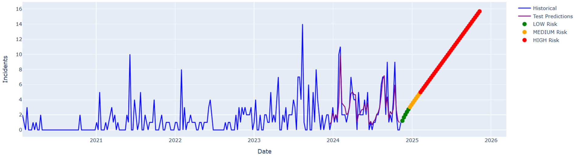
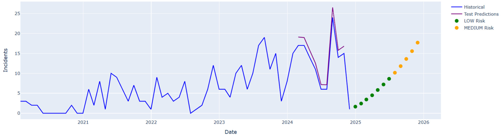
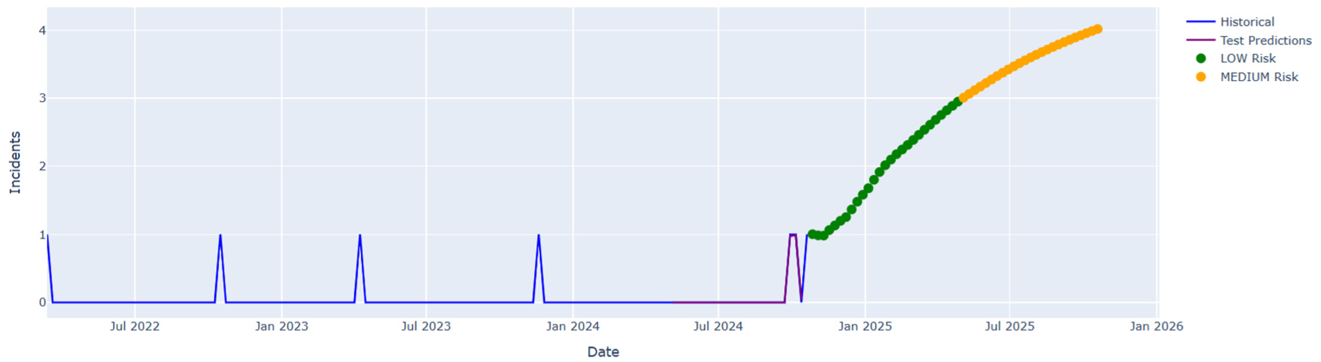
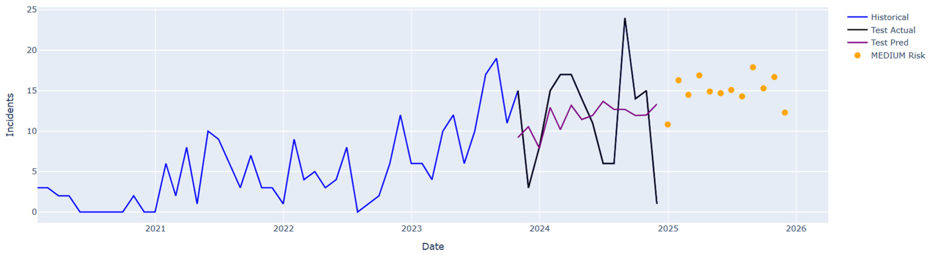
SARIMAX model: The forecasting results present CCTV failure predictions for two locations, Figures 8 to 11, through weekly and monthly forecasts. The SARIMAX model analysed historical data from these locations to create predictions for the upcoming 52 weeks (weekly) and 12 months (monthly). The forecasted data points receive risk level classifications of High, Medium, and Low according to predetermined thresholds, while the results display failure risk potential through visualisation. The visualisation used SARIMAX to predict CCTV incident failures at locations A and B, while showing future risk levels for weekly and monthly periods (Figures 8–11). The actual incident numbers are represented by the blue line in the graph, while forecasted values are shown as coloured markers indicating upcoming risk levels. The risk assessment uses green markers to indicate low-risk weeks or months, orange markers for medium-risk periods, and red markers for high-risk periods. The weekly forecast reveals periodic high-risk weeks, which indicate that proactive maintenance should occur during these times.
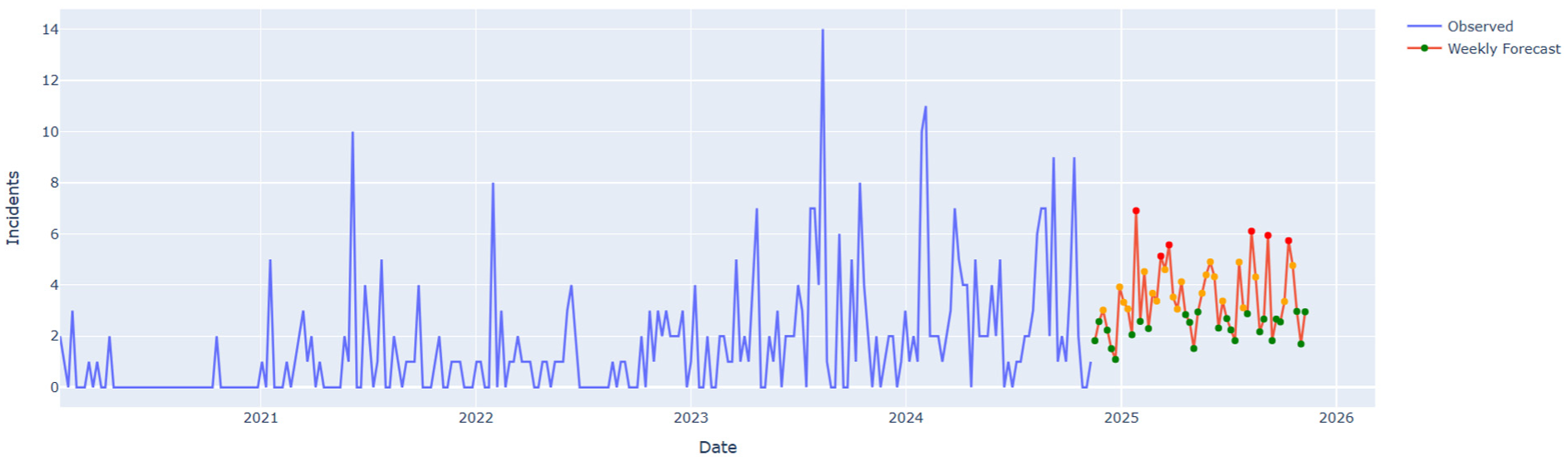
SARIMAX forecasting weekly CCTV failure for location A.

SARIMAX forecasting monthly CCTV failure for location A.
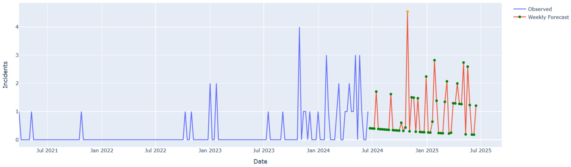
SARIMAX forecasting weekly CCTV failure for location B.

SARIMAX forecasting monthly CCTV failure for location B.
LSTM model: The LSTM model presents risk analysis and forecasting visualisations for two selected locations (A and B) in Figures 12 to 15. The weekly forecasts are presented in Figures 12 and 14, while the monthly forecasts are shown in Figures 13 and 15.
LSTM forecasting weekly CCTV failure for location A.
LSTM forecasting monthly CCTV failure for location A.

LSTM forecasting weekly CCTV failure for location B.

LSTM forecasting monthly CCTV failure for location B.
The visualisations demonstrate that the model effectively captures seasonal fluctuations and trend patterns, with forecasted risk levels closely matching historical patterns in both locations. In contrast, the monthly forecasts, although still showing good alignment with actual trends (R2 = 0.84), displayed slightly higher prediction errors, suggesting reduced precision in capturing longer-term fluctuations.
CNN model: The Convolutional Neural Network (CNN) model was applied to the weekly and monthly CCTV failure incident data to explore its ability to detect local temporal patterns and predict future incidents. In the LSTM evaluation, the CNN model was trained using the historical incident counts per location and tested on unseen data. Figures 16 to 19 present the CNN-based weekly and monthly forecasts for two locations. The plots show historical data, test predictions, and forecasted incident counts, categorised into Low, Medium, and High-risk levels. For both frequencies, the CNN model was able to capture the overall trend and seasonal variations in the data, with relatively stable short-term predictions.

CNN forecasting weekly CCTV failure for location A.

CNN forecasting monthly CCTV failure for location A.
CNN forecasting weekly CCTV failure for location B.

CNN forecasting monthly CCTV failure for location B.
ETS model: The ETS model produced inconsistent results when applied to the different datasets. The weekly forecast results showed that the non-SARIMAX model produced the lowest MSE value of 12.42 and MAE value of 2.62, which indicates good short-term prediction accuracy.
The visual risk analysis and forecasting results for the SARIMAX, LSTM, CNN, and ETS models are presented in Figures 8 to 23 for two selected locations, at both weekly and monthly resolutions. The plots display historical incident counts, along with model predictions for the test period and future forecasts, which are grouped into low, medium, and high-risk categories based on established thresholds. The visualisations show that SARIMAX generates the most predictable and stable patterns, which match actual trends, especially when using weekly forecasting. The weekly patterns in LSTM forecasts show reasonable visual accuracy, but the model produces less consistent results when predicting monthly trends. The visualisations from CNN models show larger deviations and less stable patterns, and ETS produces moderate alignment but with occasional underestimations of high-risk periods. The system demonstrates better performance because the monthly forecast shows a steady pattern by predicting only a few high-risk months. The visual representations enable maintenance teams to detect upcoming high-risk incidents, which helps them allocate resources effectively to critical weeks and months, thus reducing system downtime.

ETS forecasting weekly CCTV failure for location A.
ETS forecasting monthly CCTV failure for location A.

ETS forecasting weekly CCTV failure for location B.

ETS forecasting monthly CCTV failure for location B.
Conclusion
The research indicates that combining downtime prediction with failure forecasting results in more effective proactive maintenance of railway CCTV systems. The Bayesian Ridge regressor achieved the highest MTTR accuracy, but KNN’s under-prediction strategy proved most beneficial for operations, as it reduced the average downtime by 4.9%. The SARIMAX model demonstrated consistent performance, generating accurate and understandable forecasts for both weekly and monthly time horizons. The LSTM model demonstrated excellent weekly prediction abilities at specific locations, yet its monthly predictions were less accurate. The CNN model produced reliable predictions in particular cases, but its long-term predictions were unstable, and the ETS model delivered stable monthly forecasts with minimal predicted high-risk months. The visual risk assessment framework (Figures 8–23) helped identify essential intervention times and dangerous areas, which guided specific and prompt maintenance activities. The monthly forecasts revealed low- and moderate-risk periods, which enabled better resource management and reduced system downtime.
To enhance prediction accuracy, flexibility, and operational responsiveness, future research should investigate hybrid or ensemble forecasting techniques that integrate real-time data streams and leverage the advantages of both statistical and deep learning models. Other crucial railway subsystems, passenger bodyside doors, passenger information systems (PIS), autocouplers, TCU (Complete), AWS/TPWS, generic components (underframe-bogies), DSD/Vigilance, OTMR Units, and ACU (Complete), will also be examined in the future. A thorough, fleet-wide condition monitoring strategy will be made possible by extending the predictive framework to these assets. By using these predictive techniques, railway fleet availability, system dependability, and maintenance cost effectiveness will all be enhanced.
Footnotes
Acknowledgements
Siemens Mobility Limited UK is the sponsor of a larger study that includes this one. The authors express their gratitude to Siemens for funding this study.
Handling Editor: Chenhui Liang
Funding
The authors disclosed receipt of the following financial support for the research, authorship, and/or publication of this article: The publication article is part of a joint funded PhD studentship research project sponsored by Siemens Mobility Limited UK and Glasgow Caledonian University.
Declaration of conflicting interests
The authors declared no potential conflicts of interest with respect to the research, authorship, and/or publication of this article.