Sage Journals: Discover world-class research

Abstract

Anomaly detection in rotating machinery often faces challenges in threshold determination and false alarms, which not only restrict the generalization ability of models but also lead to unnecessary downtime. To address this issue, this study explores a probabilistic expression framework suitable for anomaly detection of rotating machinery under constant-speed and stable operating conditions. Specifically, the reconstruction error (RE) based on Variational Autoencoder (VAE) is first adopted as a health indicator. Aiming at the problems of threshold setting and false alarms in its application, a probabilistic expression framework based on RE and Kernel Density Estimation (KDE) is proposed. This framework can directly provide anomaly probability density, and distinguish between interference and anomalies by quantifying the impact of abnormal values on the shape of the probability density curve, thereby avoiding threshold dependency and the risk of false alarms. The performance of this indicator is validated using experimental data of gears and bearings. The empirical relationship between the coefficient of variation (CV) of reconstruction error and the KDE window h is analyzed and presented, and a comparative analysis with traditional methods is also conducted. The research shows that this framework does not require setting an anomaly detection threshold for reconstruction error, nor does it issue alarms for non-abnormal states, providing a new solution for anomaly detection in rotating machinery.

Keywords

probabilistic expression anomaly detection rotational machinery

Introduction

The components of rotational machinery such as gears and bearings are prone to damage due to various complex factors under operational conditions and loads. This may cause financial losses or personnel injuries. Therefore, the abnormally detection of rotational machinery is of great significance.

It is a critical issue close to practical application and essentially aims at finding a hyperplane or threshold value for anomaly detection. Domestic and international researchers have made efforts to address this issue.^1–19 Specifically, Shin et al.¹ proposed a one-class SVM (support vector machine) for hyperplane detection in high-dimensional outlier problems, with hyperparameters determined by cross-validation. The method was validated using artificial and real datasets under constant conditions, and results show its performance is mostly superior to that of MLP (multiple layer perceptrons), but it is sensitive to parameter and kernel choices. Fernández-Francos et al.² utilized a novel one-class v-SVM algorithm to determine a hyperplane for early bearing defect detection, followed by fault diagnosis via sensitivity tests and envelope spectrum analysis. Their study used only data under normal conditions for model training, where parameter v estimated spurious data in the normal state registry. The method was verified with bearing datasets under constant conditions, indicating that sensitivity tests can automatically select the vibration spectrum zone with the most evident fault, qualitatively assess its temporal evolution, and identify failure locations in early stages-though still parameter-sensitive. Sarri et al.³ summarized threshold-setting methods for fault detection (manual definition, supervised or unsupervised learning) and their shortcomings. To address these, they trained parallel one-class SVM models by adjusting input features from envelope analysis and model tuning parameters, defining system thresholds by estimating detection model accuracy. Plakias and Boutalis⁴ adapted the anomaly detection scheme of GAN (generative adversarial network) from medical images. They identified instability and predefined threshold selection as key shortcomings. Inspired by this, they proposed a GAN architecture for industrial fault detection, using feature matching to ensure stability and a search algorithm to compare discriminators by fault detection capability. Arunthavanathan et al.⁵ analyzed the pros and cons of physical, data-driven, and knowledge-based models in process system monitoring or diagnosis. They proposed a model integrating one-class SVM and neural networks to capture known fault conditions, classify them, and determine root causes. Meng et al.⁶ focused on anomaly detection of rolling bearings in wind turbines, extracted features from vibration signals using EMD, filtered effective components through a kurtosis threshold, and analyzed anomalies by combining with theoretical fault frequencies. With labeled data, they trained classifiers like KNN (incorporating hyperplane demarcation logic). Ultimately, the EMD-KNN method achieved efficient fault diagnosis, with more prominent signal features after processing. Pan et al.⁷ analyzed shortcomings of intelligent fault recognition methods and GAN limitations in addressing data insufficiency, proposing a convolutional adversarial auto-encoder for unseen fault detection, though its detection threshold is sensitive to training data, requiring manual fault type classification. Zhao et al.⁸ discussed applications of one-class support vector machine (OC-SVM), support vector data description, extreme learning machine, and variants for fault detection, addressing weighted OC-SVM shortcomings by combining distance-based and density-based weighting strategies via a trade-off parameter. Wu et al.⁹ introduced one-class classification in predictive maintenance, identifying two key issues: feature extraction relying on human experience and non-reconfigurable methods, plus some condition monitoring approaches not using one-class learning. They proposed fault-attention generative probabilistic adversarial autoencoders (GPAA) to capture low-dimensional manifolds and construct fault-related anomaly indicators, adopting a spectral energy-based fault-attention noise prior distribution to improve noise adaptability, validated via time-varying and discriminable datasets. Zhao and Huang¹⁰ highlighted class imbalance learning (CIL) issues in real-scenario data-based fault detection, describing applications of one-class classification algorithms to solve CIL. Aiming at OC-ELM’s hard margin flaw, they proposed a soft one-class extreme learning machine, allocating adaptive soft margins to training samples to enhance algorithm robustness and accuracy. Ruicong et al.¹¹ compared shortcomings of signal processing, machine learning, and deep learning for equipment fault detection, identifying two key problems in deep neural network-based methods: anomalous training dataset construction and training result transfer. Despite efforts to reduce domain deviation, they noted the ignored importance of weight parameters in classification stages for inter-domain distribution adaptation, designing an unsupervised adversarial domain adaptive network based on minimum domain spacing, introducing maximum mean difference (MMD) at the adaptation layer and classifier end to calibrate domain distribution differences twice. Pu et al.¹² reviewed prior machinery anomaly detection and classification with unlabeled data, pointing out that normal data are usually more abundant than anomaly data in real applications, causing diagnosis obstacles. They proposed a one-class generative adversarial detection framework using bi-GAN and one-class SVM to learn one-class latent knowledge for fault detection, novelty detection, and classification. Yang et al.¹³ first noted that one-class classification, binary classification, artificial neural networks, and Naïve Bayes methods are commonly used for fault detection, then introduced fault classification studies by other researchers. They concluded that collecting data for all possible abnormal conditions is infeasible, making incremental classification of unknown abnormal patterns a challenging task in machinery fault diagnosis, proposing an incremental novelty identification method: training 1-D CNN autoencoders for multi-signal feature extraction, then OS-ELM models for known conditions based on extracted features. Princz et al.¹⁴ proposed an unsupervised machine learning approach which is adopted for condition monitoring in anomaly detection of binary time series data. After preprocessing the dataset, the detection performance of models like IF, LOF, DBSCAN, k-Means, and autoencoder was evaluated using metrics such as accuracy, F1-score, and execution time, with a multi-decision fusion mechanism to enhance robustness. Results show that Isolation Forest and Local Outlier Factor models excel in precision and real-time performance, while the AutoML model achieves high accuracy but lacks real-time capability, providing a basis for model selection in industrial scenarios. Yu et al.¹⁵ proposed an unsupervised signal anomaly transformer (SAT) method to address the lack of fault samples in bearing life anomaly detection. The method optimizes the anomaly Transformer based on signal input, employs a CNN encoder-decoder structure to encode and reconstruct signals, replaces symmetric KL divergence with Wasserstein distance to measure distribution differences, and introduces a new metric to compare decoded and original signals. It achieves an average accuracy of 99.54% on simulated signals and validates the detection capability for bearing signal anomalies on real-world IEEE and XJTU-SY datasets, enhancing the accuracy and reliability of anomaly prediction without requiring fault samples. Roy et al.¹⁶ proposed a Graph Anomaly Detection via Neighborhood Reconstruction (GAD-NR) model to address the limitation of traditional Graph Autoencoders (GAE) to address the limitation of traditional Graph Autoencoders (GAE), which only focus on direct link reconstruction. It uses a GNN encoder to extract node representations, and the decoder reconstructs node neighborhood information (self-attributes, connection patterns, neighbor attributes), optimizing the reconstruction loss via Gaussian approximation of neighborhood feature distributions and KL divergence calculation. On six real-world datasets, AUC is improved by up to 30% compared to baselines, effectively detecting contextual, structural, and joint-type anomalies with higher computational efficiency than traditional methods. Lu et al.¹⁷ proposed a method based on signal transform and memory-guided multi-scale feature reconstruction for anomaly detection in non-stationary rotating machinery. Vibration signals are transformed into time-frequency maps via wavelet transform, combined with a composite scaling feature extraction network (EfficientNet) and multi-scale memory modules to constrain the decoder’s reconstruction ability for distinguishing normal and abnormal samples. It outperforms traditional methods in detection accuracy and robustness on loader gearbox and variable-speed bearing datasets, effectively reducing false alarm rates and adapting to complex working conditions. Choi et al.¹⁸ designed a Frequency-Enhanced Network (FENet) for anomaly detection in hydraulic piston pumps, integrating self-supervised learning to address detection challenges under variable conditions. The method introduces Frequency-Aware Convolution (FAC) and Rotary Position Embedding (RoPE) to capture frequency-domain features and temporal dependencies, constructs a robust model via CutMix data augmentation and multi-decision fusion (IF, OCSVM, EE), and proposes an MD-FDR health index to optimize fault severity assessment. It accurately identifies slipper wear faults in industrial pump experiments, reducing false alarm rates and demonstrating significant health index effectiveness. Zhu et al.¹⁹ presented an online detection model for early rolling bearing faults based on a deep attention convolutional autoencoder (DACAE) and multi-decision fusion to address noise interference under variable conditions. An improved multi-head attention mechanism is designed with rotary position embedding, and a self-supervised pre-training and target-domain fine-tuning strategy is combined with data screening, using multi-algorithm voting (IF, OCSVM, EE) for noise-resistant detection. It achieves early fault localization on the IMS dataset with a lower false alarm rate than single algorithms, suitable for variable-condition environments. Liu et al.²⁰ proposed an anomaly detection method for machinery under time-varying operating conditions based on state-space and neural network modeling. The method models the health state, operating conditions, and response signals via a state-space model, parameterizes their relationships using the nonlinear fitting capability of neural networks, updates parameters alternately with the extended Kalman filter, constructs detection indicators based on real-time neural network parameters, and validates its effectiveness through rolling bearing experiments.

Though many researchers have made much efforts to determine the hyperplane or threshold in anomaly detection, some deficiencies of these methods can not be ignored. Specifically, it mainly includes the following aspects:

(1) Strong parameter dependence and insufficient robustness. Most methods (e.g. one-class SVM, GAN, autoencoders) are highly sensitive to hyperparameters and model architectures.

(2) Lack of dynamic adaptability in threshold determination. In practical applications, finding an appropriate hyperplane or threshold for anomaly detection is a crucial issue, and existing methods have shortcomings in determining the threshold.

(3) High false alarm rates and inadequate resistance to noise or operational interference. Noise interferes with reconstruction-error-based methods, often misclassifying strong noise as anomalies.

Against the above challenges, some researchers have introduced adversarial concepts and conducted research in the fields of power systems and rotating machinery.^21–24 For instance, to tackle the lack of dynamic adaptability in threshold determination, Wang et al.²³ proposed a threshold-free unsupervised framework that employs a GAN structure: the generator models the distribution of normal data to generate synthetic normal signals, while the discriminator integrates multi-module features for classification. Rather than relying on manually set thresholds, this framework directly outputs probabilities corresponding to healthy, fault alarm, or fault states. This enables it to dynamically adapt to changes in data distribution and overcome the limitations of fixed thresholds in complex scenarios. Hiranaka and Tsujino²⁴ focused on the issues of ‘high false alarm rates and inadequate anti-interference capability’. Their research addresses speed-induced signal fluctuations (noise-like interference) by incorporating rotational speed as a conditional input into the Variational Auto-encoder (VAE). The model adaptively learns normal patterns under varying speeds, and employs strategies such as interpolation and extrapolation for unseen speed conditions and limiting the number of training samples per speed. These measures enhance the model’s resistance to dynamic operational interference, thereby reducing false alarms caused by speed fluctuations. The findings of these studies hold significant reference value for future research. In this study, research is carried out to mainly address the threshold determination and false alarm issues from another perspective. Inspired by References 7, 9, and 19, an existing health indicator, reconstruction error based on VAE, is utilized as a basic indicator. An and Cho²⁵ suggests reconstruction probability outperforms RE, but our experiments show the opposite, hence RE is prioritized. Therefore, it will no longer be discussed in this study. The core advantages of using reconstruction error as an anomaly detection metric lie in its theoretical soundness, computational efficiency, and adaptability to unlabeled data. Rooted in generative modeling, it assumes normal data can be accurately reconstructed, while anomalies yield significant errors due to their deviation from learned distributions. This makes it inherently suitable for unsupervised scenarios where abnormal samples are scarce, as it only requires normal data for training. Additionally, reconstruction error offers a straightforward quantitative measure that avoids complex feature engineering, enabling real-time monitoring. Its dynamic adaptability-via online model updates-allows it to accommodate gradual shifts in normal patterns, while multi-modal compatibility supports applications across images, time-series, and text. This combination of theoretical rigor and practical feasibility has established reconstruction error as a cornerstone of modern anomaly detection. However, in practical application, a reconstruction error curve is always fluctuating, and sensitive to the running state of the machinery, thus it is difficult to determine a threshold and avoid wrong warning. Therefore, to address these issues, this study proposes a threshold-free framework by integrating RE and KDE,²⁶ leveraging probability distribution characteristics to distinguish states. Eventually, anomaly detection is realized without a threshold and wrong warning. However, this study’s core innovation lies not in algorithmic innovation, but in proposing a solution framework to tackle practical problems (e.g. threshold setting and false alarms) via probabilistic expression, and establishing criteria for distinguishing normal, interfering, and abnormal states.The main contributions are as follows.

(1) This study proposes a probabilistic expression framework for anomaly detection of rotational machinery based on variational autoencoder (VAE) reconstruction error and kernel density estimation (KDE), This framework can directly provide anomaly probability density, and distinguish between interference and anomalies by quantifying the impact of abnormal values on the shape of the probability density curve, thereby avoiding threshold dependency and the risk of false alarms.

(2) Based on the impact of abnormal values on the probability density curve, a quantitative judgment logic for normal, interference, and abnormal states has been analyzed and established. Additionally, through experimental analysis, the empirical relationship between CV and h has been provided.

The remaining part of this article is organized as follows. The basic theory of RE and KDE is introduced in Section ‘Fundamental theories’. The probabilistic expression and specific steps for anomaly detection of rotational machinery are presented in Section ‘The anomaly detection of rotational machinery’. Two experimental cases and discussions are conducted in Section ‘Experimental validations’ and Section ‘Results and discussion’. A conclusion is shown in Section ‘Conclusions’.

Fundamental theories

Basic theory of reconstruction error

In this study, the reconstruction error (RE) based on the Variational Autoencoder (VAE) is adopted as a health indicator (HI). Below is an explanation of the underlying theory.

A VAE is a probabilistic generative model that integrates variational inference with deep learning, comprising an encoder and a decoder. The encoder maps input data to a latent space distribution, capturing the probabilistic relationship between the data and latent variables. The decoder then maps the latent space back to the original data space, attempting to reconstruct the input. Specifically, a VAE models an approximate posterior distribution fϕ (z|x) of the latent variable z given the input x. The decoder models the likelihood g_θ (x|z), which is the probability of the input x given the latent variable z.

Unlike deterministic traditional autoencoders, the VAE models the distribution of latent variables rather than fixed values, enabling probabilistic modeling of the reconstruction process.

The reconstruction error in VAE is derived from the discrepancy between the original input and its probabilistic reconstruction. Distinct from traditional autoencoders (which use deterministic pixel-wise error metrics), VAE-based RE incorporates two key features: probabilistic quantification and uncertainty awareness. RE in VAE is linked to the reconstruction discrepancy, defined as the expected difference between the original input and the reconstructed output. This measures how well the original input can be reproduced from the learned latent distribution, with higher RE indicating higher anomaly likelihood. For normal data, RE is low (consistent with the learned distribution), while anomalies yield high RE due to deviation from the learned patterns. RE is calculated as the mean squared error between original and reconstructed signals (1), where L denotes the number of data points, xi denotes original data, and ${\hat{x}}_{i}$ denotes reconstruction data.

RE = \frac{1}{L} \sum_{i = 1}^{L} (x_{i} - {\hat{x}}_{i})^{2}

(1)

During anomaly detection, the VAE is trained only on normal data. After training, the reconstruction error is computed for each data point in the test set. By being trained on normal data, the VAE learns the distribution of healthy states. Test data with high RE are flagged as anomalies, as they are unlikely to conform to the learned normal distribution.

Basic theory of kernel density estimation

Kernel density estimation (KDE) is a non-parametric method for estimating the probability density function (PDF) of a random variable from a finite data sample. Unlike parametric approaches (e.g. assuming a Gaussian distribution), KDE does not require prior knowledge of the data’s underlying distribution. Instead, it constructs a smooth density function by aggregating local information around each data point. The estimated density at a point x is given by (2), where x_j (j = 1, 2, …, n) represents observed data points, K(·) is a kernel function that determines the shape of the distribution around each data point, h denotes bandwidth (a smoothing parameter) that controls the the trade-off between bias and variance, and n is the number of data samples.

\hat{p} (x) = \frac{1}{n h} \sum_{j = 1}^{n} K (\frac{x - x_{j}}{h})

(2)

For a kernel function, it must satisfy two conditions, non-negativity and normalization shown in (3).

K (u) \geq 0 and \int_{- \infty}^{\infty} K (u) du = 1

(3)

Common kernel functions include the Gaussian Kernel, Uniform Kernel, and Epanechnikov Kernel. The Gaussian Kernel has strong smoothness and is suitable for continuous data, and its formula is presented as (4). The Uniform Kernel is simple but less smooth, and its formula is shown as (5). The Epanechnikov Kernel has optimal efficiency, and its formula is presented as (6).

K (u) = \frac{1}{\sqrt{2 π}} e^{- u^{2} / 2}

(4)

K (u) = \frac{1}{2} I (| u | \leq 1)

(5)

K (u) = \frac{3}{4} (1 - u^{2}) \cdot I (| u | \leq 1)

(6)

The probability density curve calculated by KDE (Kernel Density Estimation) is a non-parametric estimation of the underlying probability distribution behind the data samples. Its core meaning lies in intuitively presenting the distribution density of data in different value intervals. The horizontal axis of the curve corresponds to the range of data values, and the vertical axis represents the probability density value at that point. The higher the ordinate value (density value) at a specific point on the curve, the denser the data points are around the corresponding abscissa value. More broadly, the higher the curve is in a certain interval, the denser the data is distributed in that interval, meaning that when randomly sampling, the possibility of obtaining values within that interval is greater; conversely, the flatter or lower the curve is, the sparser the data is distributed in the corresponding interval, and the smaller the probability of taking values there. This smooth curve can more truly reflect the overall distribution characteristics of the data.

However, disturbances (such as noise) and clusters of extreme values (such as anomalies) can distort the shape of the KDE curve: disturbances may cause unnecessary bulges in edge regions or make the curve rough overall, obscuring the main distribution characteristics; clusters of extreme values, on the other hand, may form false secondary peaks (e.g. a unimodal distribution being misjudged as bimodal) or stretch the tail of the curve, overestimating the tail weight and masking the true dispersion of the data. All these will cause the curve to deviate from the true underlying distribution of the data and interfere with the judgment of core features (such as peaks and distribution patterns). Conversely, disturbances and anomalies can also be detected through the analysis and quantification of such features.

In this study, three indicators, presented in Table 1, are adopted to feature the curves and describe their changes.

Table 1.

Definitions of indicators.

Indicators	Core meaning	Formula	Calculation basis
Height of main peak	The core peak of the KDE curve reflect the aggregation intensity of the data at this position	$f (x_{peak})$	KDE curve
Standard deviation	The average degree to which data deviates from the mean	$σ = \sqrt{\frac{1}{m} \sum_{i = 1}^{n} {(x_{i} - \bar{x})}^{2}}$	{x₁, x₂, …, x_m}
Range	the curve width corresponding to 0.5% of the main peak height	$x_{right} - x_{left}$	{x₁, x₂, …, x_m}

Note. f (*) denotes the function of KDE curve; $x_{peak}$ : the abscissa position corresponding to the main peak.

{x₁, x₂, ⋯, x_m} denotes KDE curve data, m represents the amount of KDE curve data.

$\bar{x} = \frac{1}{m} \sum_{i = 0}^{n} x_{i}$ ; $x_{right}$ denotes x that the right end of the curve width; $x_{left}$ denotes x that the left end of the curve width.

Besides, the bandwidth h is the most critical hyperparameter in KDE. A large h may cause over-smoothing, leading to high bias, while a small h may result in under-smoothing, introducing noise.

In this study, kernel density estimation (KDE) is combined with a dynamic sliding window to calculate the relative change rate of the characteristic parameters of the window curve, which is used for the anomaly detection and evaluation of rotating machinery.

The anomaly detection of rotational machinery

In this study, we propose an anomaly detection method for rotational machinery (such as gears and bearings) by integrating reconstruction error and KDE. The entire process is shown in Figure 1 and consists of two main steps: model training and anomaly detection.

Figure 1.

The framework of the proposed method.

For the first step, signals of a healthy state are collected to train the model. Subsequently, online raw signals are fed into the trained model to obtain a reconstruction error series. For the second step, an anomaly detection model is built using KDE where h and s are bandwidth and sliding distance. The RE series are input into this model to detect anomalies in the rotational machinery.

Next, two subsections elaborate on these two steps in more detail.

Model training and RE series construction

In this section, two modules are included to train the model and obtain RE series, as shown in Figure 2.

Figure 2.

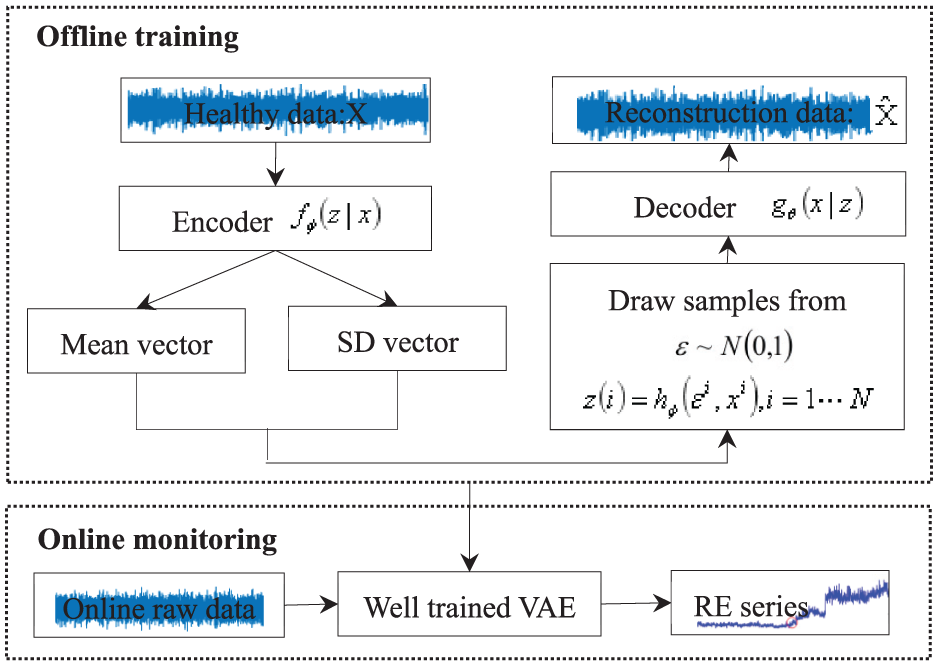
Model training and RE series construction.

Specifically, raw vibration signals in a healthy state are used to train the model, enabling the decoder to reconstruct the original signals with a small reconstruction error. Then, online data are fed into the well-trained model, and the RE series are taken as health indicators. When anomalies occur, the corresponding RE indicator will increase and deviate from the normal RE series as the anomaly progresses. This shows a positive relationship between RE and the severity of the anomaly, reflecting the occurrence and development of the anomaly. Hence, we take RE as an HI for rotational machinery.

The online raw signals are fed into the trained model. The decoder reconstructs the signals and outputs a corresponding RE indicator. An RE indicator reflects how successfully the decoder can reconstruct the input signals: a larger value means a greater reconstruction error between the input and output.

Anomaly detection model based on KDE

During the service life of rotating machinery, abnormal phenomena usually occur gradually. The reconstruction error (RE) sequence often shows fluctuations in the early stage and then gradually deviates from the average level. If a false alarm triggers an unplanned shutdown, it will lead to severe waste of resources and production interruption-not only causing ineffective consumption of human and material resources, but also likely leading to misjudgment in predictive maintenance strategies, resulting in premature replacement of components or missed detection of real faults. To accurately evaluate the operating status of equipment and avoid the risk of misjudgment, this study introduces Kernel Density Estimation (KDE) in the final stage. It constructs a probabilistic criterion by calculating the probability density distribution of the RE sequence, and proposes a more robust state discrimination rule based on its dynamic changes.

As we all know, the degradation process is a non-stationary stochastic process. In essence, a stochastic process is non-stationary if its statistical characteristics change over time. Specifically, statistical quantities such as the mean function, variance function, and autocorrelation function of this process change with time and lack temporal stability. The sliding window in Kernel Density Estimation (KDE) mainly serves two purposes: first, to determine the data range for kernel function calculation; second, to control the smoothness of the estimation results. By calculating the probability density of the reconstruction error (RE) sequence within the window and analyzing the morphological changes of the curve, we can infer the operating state of rotating machinery. The input of KDE is the data samples used for estimation and relevant parameter settings, and the output is the estimated value of the data’s probability density function (PDF).

Specifically, data samples are the basic input of KDE, which are a set of observed data points from an unknown distribution, and they can be either one-dimensional or multi-dimensional. Generally speaking, the more data samples there are and the better their representativeness of the overall distribution, the more ideal the estimation effect of KDE will be. The reconstruction error (RE) sequence will be input into the KDE model.

In addition, the kernel function determines how to weight the probability density around each data point in the reconstruction error (RE) sequence. Common kernel functions include the Gaussian kernel function, Epanechnikov kernel function, and uniform kernel function. For RE data that usually exhibit continuous and smooth fluctuation characteristics during mechanical degradation, the Gaussian kernel function is particularly suitable. Therefore, in this study, the Gaussian kernel function is adopted.

Finally, the bandwidth is a critical input parameter in KDE, controlling the smoothness of the kernel function. The bandwidth size significantly affects the result of the KDE estimate. A smaller bandwidth will make the estimated result closer to the original data points, potentially leading to an overly fluctuating estimate with excessive local details. Conversely, a larger bandwidth will yield an overly smooth estimate, possibly causing the loss of some real features of the data. In this study, this parameter will be given a suitable selection based on experimental analysis, which will be presented in Section ‘Results and discussion’.

In general application, KDE consists of three layers which are input layer, sampling layer, and output layer. The input layer has a number of points the same as the length of the sliding window. For example, assume the length is k, then the input sample is like $x = {x_{1}, x_{2}, \dots, x_{k}}$ . A mapping relationship is established between the input layer and sampling layer, and make $x$ to be $y = {y_{1}, y_{2}, \dots, y_{m}}$ . The output layer calculate the conditional probability density function (PDF) of the points within the current window by formula (7), where $p (y_{i} | X)$ represents the value of the conditional PDF at the sampling point $y_{i}$ , $K (x_{j}, y_{i})$ is the kernel function, and h is the bandwidth.

p (y_{i} ∣ X) = \frac{1}{k h} \sum_{j = 1}^{k} K (x_{j}, y_{i}) i = 1, 2, \dots, m

(7)

The whole procedure of proposed framework for abnormally detection of a rotational machinery under constant speed is presented in the block diagram in Figure 3. The specific steps are described as follows:

(1) Model training with normal data: first, a VAE model is established and trained using normal data. Through this step, a well-trained model and a RE series are obtained. In addition, the CV value is calculated based on the normal data to determine the fluctuation range of the relative change rate of KDE curve parameters. This model, RE series, and related parameters can be used for subsequent processing of online data.

(2) KDE probability density calculation: with reference to the CV value, the KDE window width h is determined, and the specified parameter features of the probability density curve of the reconstruction error in the normal state within the window are calculated. The online data is fed into the well-trained model to obtain new reconstruction error values. The window is moved to cover the new reconstruction error values, and the specified parameter features of the probability density curve of the new window as well as the relative change rate are calculated.

State discrimination: the state corresponding to the window is determined according to the judgment criteria.

Figure 3.

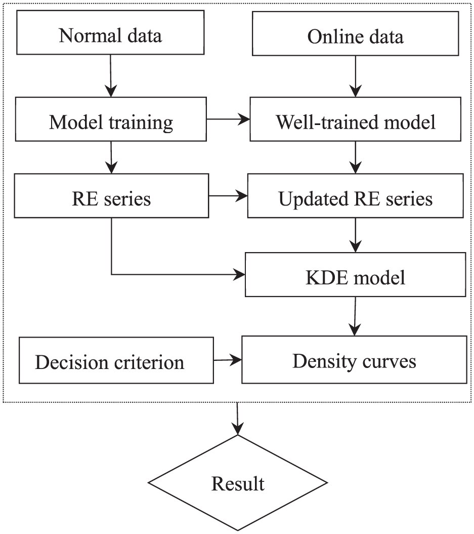
A block diagram of the proposed framework.

Experimental validations

Though components like bearings or gears are prone to damage due to various complex factors under operation circumstances and loads in real applications, it still often takes a relative long time to collect real data. Therefore, our proposed method is verified by two experimental systems, where public run-to-failure experiments data of gear and bearing under constant speed are from the University of New South Wales (UNSW), and the Joint Laboratory of Xi’an Jiaotong University and ShengYang Company (XJTU-SY). The websites are attached below and accessed on 27 Jun 2025. Eventually, we carried out two case studies and discussed the results.

(UNSW: https://data.mendeley.com/datasets/p2yryg9k6z/2; UNSW: https://data.mendeley.com/datasets/h4df4mgrfb/3)

Case study 1

In case study 1, a run-to-failure test (with and without lubrication) was conducted on the spur gearbox test rig of UNSW, and the lubricated test experiment data set of gear is used. The gearbox system consists of a motor, gearbox, brake, and signal acquisition system, which is presented in Figure 4. Specifically, a torque meter is utilized to connect a 4-kW motor and the input shaft of the gearbox through couplings. An electromagnetic particle brake (EMP) used as a load facility is connected to the output shaft. A pinion installed on the input shaft drives a gear on the output shaft through meshing motion. To accelerate the wear rate, the two gears are made of mild steel (JIS S45C). Besides, two encoders are connected to the remaining free ends of the input and output shafts by couplings respectively.

Figure 4.

The gearbox test rig of UNSW: (a) physical overall view of the system, (b) local view of the gearbox with two accelerometers, and (c) a schematic diagram of the system.

The specific parameters of the gearbox are listed in Table 2. The test endured approximately 67 h and 16 min (equivalent to around 3.25 million running cycles of the input shaft). The input shaft speed is fixed to 16 Hz while the brake load is 20 Nm.

Table 2.

Gear parameters.

Spur gear	Number of teeth
Pinion (driving gear)	19
Gear (driven gear)	52

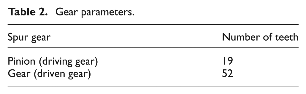
Vibration signals were collected at regular intervals (approximately every 5 min) with a sampling frequency of 100 kHz for a duration of 11 s, and description of sensors is listed in Table 3. For the lubricated test, the test rig was halted roughly every 0.1 million cycles to record the surface condition using the molding technique.

Table 3.

Accelerometer sensitivity.

Type	Sensitivity (mV/ms⁻²)	Symbol in dataset
B&K 4396	10.0	Vib1
B&K 4394	1.0	Vib2

In our study, only ‘vib1’ is utilized for analyzing. For convenience, the ‘vib1’ signal is resampled at a new sampling rate of 5120 Hz. Thus, we obtained 10 data sets, each of which has 56,320 points in it and four selected datasets are presented in Figure 5. Then, more samples were obtained by dividing each set into segments. Given each segment has 2560 points, the total samples will be 220. Eventually, all the samples are divided into training samples and testing samples. Sine the samples cover the entire run-to-failure period, the selection of training samples can not be random. It is necessary to strictly follow the chronological order while used.

Figure 5.

Experimental signals of case 1.

According to prior knowledge, the first five datasets are considered to correspond to the normal operating state. Starting from the sixth dataset, anomalies gradually emerge and become severe. Therefore, the number of training samples is generally less than 110. In this case, the applied model VAE is initialized with parameters listed in Table 4, which are referenced in Zhao and Feng.²⁷

Table 4.

Initial parameters of VAE model establishment.

Input	input_dim = 2560, latent dim = 2, batch size = 32, learning_rate = 0.001, iterations = 1000
Modules	Number of neurons
Encoder	Input layer		Hidden layer 1	Hidden layer 2	Output layer
	2560		128	64	Mean	Log_var
			Re LU	Re LU	2	2
Decoder	Input layer		Hidden layer 4	Hidden layer 5	Output layer
	Mean	Log_var	64	128	2560
	2	2	Re LU	Re LU

Note. input_dim: dimension of input sample; batch size: number of samples fed to the model for one time; iterations: number of repeats for the entire model; Activation: Re LU; Mean: mean; Log_var: the logarithm of the variance.

Figures from Figure 6 present reconstruction error curves with different training set configuration. From the perspective of these reconstruction error curves and the anomaly detection scenario, the following aspects such as anomaly occurrence patterns and trends as well as impact of training set configuration can be illustrated.

Figure 6.

Reconstruction error curves: (a) 2 training datasets, 44 training samples, 176 testing samples, (b) 3 training datasets, 66 training samples, 154 testing samples, (c) 4 training datasets, 88 training samples, 132 testing samples, and (d) 5 training datasets, 110 training samples, 110 testing samples.

Firstly, the circles mark the positions where anomalies start to emerge. Among different sub-figures (corresponding to different numbers of training datasets and sample division situations), the anomalies do not occur at exactly the same sample points. However, as a whole, with the progression of the sample sequence, there is a transition from a normal state (low error, stable) to an abnormal state (sudden error change, increased fluctuation). For example, in (a), there are abnormal points around sample points 20, 40, and 120. In (b), (c), and (d), there are also small abnormal fluctuations at relatively early sample points, followed by more significant anomalies later. This indicates that the system or data generation process gradually evolves from a normal state to an abnormal state, and the anomaly may have a process of ‘early signs-significant outbreak’. Secondly, in the normal operation stage (before the anomaly), the reconstruction error is generally at a low level and relatively stable. For example, in (a), the error of most sample points is close to 0. In (b), (c), and (d), the error in the normal stage also fluctuates around a reference value. After the anomaly occurs, the error rises and the fluctuation intensifies, reflecting that the data characteristics, system operation mode, etc. have changed significantly from the normal state. This may be caused by factors such as the development of equipment failures (from initial minor anomalies to enlarged failures) and interference in data collection.

Besides, for Figure 6(a), the distribution of abnormal points in the error curve is relatively scattered, and there are high-error points with large sudden changes. This may be because the number of training samples is small, and the model does not learn the normal mode of the data sufficiently. The recognition of anomalies and the characterization of errors are obvious in extreme cases (large anomalies), but the capture of early small anomalies may be insufficient (or it can be said that early small fluctuations are easily judged as normal, and only later large anomalies are prominent). For Figure 6(b) and (c), as the number of training datasets increases and the number of training samples becomes larger, the early small anomalies marked by red circles are clearer. This shows that more training data enables the model to learn more detailed normal modes, and can identify the initial signs of anomalies (small error fluctuations) earlier. At the same time, the overall error curve has a more regular fluctuation after the anomaly compared to (a), and the model can characterize the development process of the anomaly more continuously. For Figure 6(d), as the number of training samples further increases, the small error fluctuations at the starting points of anomalies are accurately marked, and the error curve in the significant stage of the anomaly development is also smoother (compared to (b) and (c)). This indicates that sufficient training data makes the model’s representation of the normal mode more accurate, the sensitivity of anomaly detection and the ability to track the development process of the anomaly are stronger. From the initial anomaly signs to the significant occurrence of the anomaly, the characterization of the error change is more delicate.

However, the boundary between normal fluctuations and abnormal errors is ambiguous. Error distributions vary significantly under different training configurations (e.g. abrupt error changes with few samples vs gradual trends with more samples). Fixed thresholds often misclassify normal fluctuations. Noise in industrial data can trigger false alarms, exacerbating the challenge of balancing sensitive detection with false alarm reduction.

Case study 2

In case study 2, the second run-to-failure experiment data set is collected from a bearing system of UNSW, as shown in Figure 7, is employed. The test rig system is composed of a motor, supporting bearings, a testing bearing, a strain gauge bridge, and auxiliary components like a coupling, encoder, and hydraulic load system, presented in the schematic diagrams.

Figure 7.

The bearing test rig of UNSW: (a) physical overall view of the system and (b) a schematic diagram of the system.

Specifically, a motor supplies rotational power to drive the shaft system and connects to the rotating shaft via a coupling to ensure stable torque transmission. Supporting bearings-such as the cylindrical roller bearing and back-to-back angular contact bearings in the schematic-stabilize the shaft and reduce radial and axial runout during rotation. The testing bearing is the core component for experiments, with its operating state (e.g. vibration, strain) monitored to analyze performance under load. A strain gauge bridge is installed near the testing bearing to measure mechanical signals (e.g. strain, deformation) and capture real-time response data. Additional components include an encoder connected to the free end of the shaft for speed and motion parameter measurement and a hydraulic load system (shown in the dashed box) that applies controlled load to the testing bearing to simulate real-world working conditions (e.g. variable force, pressure). To accelerate wear testing or simulate specific failure modes, the testing bearing and its assembly are designed to mimic industrial operating environments. The motor, couplings, and supporting bearings cooperate to maintain stable rotation, while the strain gauge bridge and encoder enable high-precision data acquisition for subsequent analysis of bearing health and failure characteristics.

The specific parameters of the test bearing are listed in Table 5. Data of four experiments are stored in four folders respectively which are named Test 1 to Test 4. There two subfolders in each folder, one has all collected signals at 6 Hz, and the other has selected samples at four speeds (6, 12, 15, 20 Hz). In this study, signals collected at 6 Hz in Test 1 and denoted as ‘accV’ are used to verify the proposed model. According to dataset information, the signals are collected at a sampling frequency of 51,200 for 12 s. The size of the datasets are 80 × 614,400.

Table 5.

Bearing parameters.

Parameters	Values
Model number	Nachi 6205-2NSE9
Type	Single-row deep groove ball bearing
Bearing pitch diameter	39.04 mm
Ball diameter	7.94 mm
Contact angle	0°
Number of balls	9

For convenience, the ‘accV’ signal is resampled at a new sampling rate of 5120 Hz. Thus, we obtained 80 data sets, each of which has 61,440 points in it and four selected datasets are presented in Figure 8. Similarly, more samples were obtained by dividing each set into segments. Given each segment has 2560 points, the total samples will be 1920. Eventually, all the samples are divided into training samples and testing samples. The same as case 1, the selection of training samples can not be random. It is necessary to strictly follow the chronological order while used.

Figure 8.

Experimental signals of case 2.

According to prior knowledge, the first 50 datasets are considered to correspond to the normal operating state. Starting from the 51st dataset, anomalies gradually emerge and become severe. Therefore, the number of training samples is generally less than 1200. In this case, the applied model VAE is also initialized with parameters listed in Table 4.

Figures from Figure 9 also present reconstruction error curves with different training set configuration. And the situations described in Figure 9 are similar to those shown in Figure 6.

Figure 9.

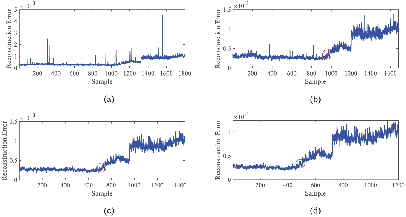
Reconstruction error curves: (a) 5 training datasets, 120 training samples, 1800 testing samples, (b) 10 training datasets, 240 training samples, 1680 testing samples, (c) 20 training datasets, 480 training samples, 1440 testing samples, and (d) 30 training datasets, 720 training samples, 1200 testing samples.

Results and discussion

Case study 1

Eventually, the RE series corresponding to Figure 6(c) are analyzed in this section. Specifically, for Figure 6(c), it presents 132 samples, that is, the RE series have 132 data points. It is worth to mention that in this study, only the states of normal, interference, and anomaly are determined, without judging the degree of anomaly. According to Figure 6(c) and prior acknowledge, from 1 to 44 data points corresponds to normal state while there is an obvious interference at 37, and starting from 45th data point, the anomaly happens. The goal of this research is to detect the existence of interference and the occurrence of anomalies.

To quantify the changes in the KDE curve, first, it is necessary to determine the window width h of the KDE in Case 1, so as to perform the calculation. By comparing Figures 6 and 9, it is found that the reconstruction error curves differ in terms of fluctuation and dispersion. Therefore, when determining the value of h, the inherent characteristics of the data need to be considered. Here, the coefficient of variation (CV), shown as (8), is used to quantify the fluctuation of the data, where σ represents the standard deviation of the data, reflecting the absolute degree of dispersion of the data, and μ represents the mean (arithmetic mean) of the data, reflecting the central tendency of the data.

CV = \frac{σ}{μ} \times 100 %

(8)

Randomly select five groups of data in normal state, with each group containing 22 data points, to calculate the average value of the coefficient of variation (CV) which finally is 3%. In order to establish an empirical relationship between CV and h, it is also necessary to define indicators for curve changes, then conduct cross-experiments, and analyze based on the conditions of the indicators.

As shown in Figure 10, assume that window width is 21 (about 7-fold the CV value 3), 10 subplots are obtained.

Figure 10.

Density curves of case 1.

As can be seen from Figure 10, windows without tail bulges (such as Curve 36) have probability density curves that are closer to a ‘single-peaked, sharp’ morphology, with data highly concentrated around a core value. This indicates that the data within such windows is more stable and adheres to conventional distribution patterns, which in turn results in more consistent model reconstruction outputs. The density curves of these windows exhibit high and narrow peaks, signifying low data dispersion. This reflects minimal fluctuations in the model’s reconstruction error for these samples, leading to more predictable output results, and also indicates greater stability in the data itself or the model’s fitting to conventional samples.

When a window contains inflection points (such as Curves 37–44), its probability density curve (with slight bulges near the peak) tends to be more ‘complex’ and the distribution may be more dispersed. This indicates that inflection points will introduce abnormal data fluctuations, disrupt the conventional distribution, and lead to an increase in the dispersion degree of data within the window. Outliers will disperse the ‘weight’ of the kernel function. KDE (Kernel Density Estimation) places a kernel function (such as a Gaussian kernel) on each data point and superimposes them to obtain the overall density curve. The kernel function of an outlier will form a small peak in the area far from the main peak. Since the total ‘energy’ of the kernel function is limited (or affected by the bandwidth), outliers will divert a portion of the weight, resulting in a reduction in the sum of the superimposed kernel functions in the main peak area, thereby lowering the height of the main peak.

Specifically, the change rates of indicators are listed in Table 6 for Curve 36–40 and Curve 44. By observing the distortion degree of multiple groups of adjacent windows (such as Curves 36–44), it can be found that from Curve 36 to Curve 37, the peak height decreases by 78.61% relatively, the dispersion degree increases by 251.61%, and the relative change rate of the curve range is 122.86%. However, from Curve 37 to Curve 44, the relative change rates of various parameters of the curves are all close to 0. This indicates that when the window moves from Curve 36 to Curve 37, an outlier occurs; while the subsequent parameters of the curves basically do not change, which means that as the window moves, no new outliers enter the window, so the outlier generated just now is an interference.

Table 6.

Change rates of indicators of curve 36–44 for case 1.

Indicators	Curve 36 and 37 (%)	Curve 37 and 38 (%)	Curve 38 and 39 (%)	Curve 39 and 40 (%)	Curve 40 and 44 (%)
Peak height relative change rates	−58.45	−2.52	−0.95	0.32	1.22
Standard deviation relative change rates	185.21	1.40	0.13	0.05	1.79
Range relative change rates	69.88	2.84	0.69	−0.69	0.69

Note. $relative change rate = (A - B) / \min (A, B)$ . A denotes the current indicator value, B denotes the adjacent previous value.

Relatively, the relative change rates of each curve parameter from Curve 44 to Curve 48 are shown in Table 7. This indicates that when the window moves from Curve 44 to Curve 48, outliers occur, and as the window moves, new outliers enter the window, so it can be judged that an anomaly has occurred. According to above explanation and description, it can be found that Curve 3 and 24 to 34, their variations are caused by interference. According to Figure 12, it can be determined that anomalies start to gradually appear from Curve 35 onwards.

Table 7.

Change rates of indicators curve 44–48 for case 1.

Indicators	Curve 44 and 45 (%)	Curve 45 and 46 (%)	Curve 46 and 47 (%)	Curve 47 and 48 (%)
Peak height relative change rates	−9.07	−8.15	−14.00	−7.35
Standard deviation relative change rates	4.88	3.21	10.01	2.03
Range relative change rates	91.10	1.43	4.59	1.01

Note. $relative change rate = (A - B) / \min (A, B)$ . A denotes the current indicator value, B denotes the adjacent previous value.

This indicates that as the window moves from Curve 44 to Curve 48, the height of the main peak of the curve is continuously decreasing, the standard deviation of the curve is increasing, and the IQR is also increasing. This shows that the dispersion degree of the data distribution is systematically and acceleratingly expanding, and such expansion has the characteristic of dynamic enhancement. Therefore, it can be judged that outliers have occurred, and as the window moves, new outliers are entering the window, which means an anomaly has occurred.

Case study 2

Eventually, the RE series corresponding to Figure 9(c) are analyzed in this section. Specifically, for Figure 9(c), it has 1440 samples, that is, the RE series have 1440 data points. Similarly, the average value of the coefficient of variation (CV) 9%. Assume that window width is 63 (about 7-fold the CV value 9). As shown in Figure 11, eight subplots are obtained and the same five indicators are also adopted to feature the curves and describe their changes.

Figure 11.

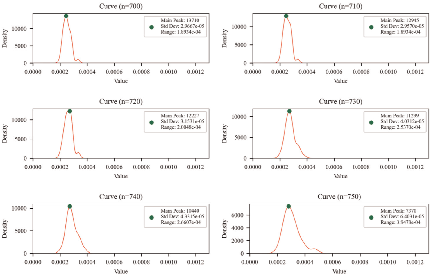
Density curves of case 2.

The relative change rates of each curve parameter from Curve 700 to Curve 750 are shown in Table 8.

Table 8.

Change rates of indicators for case 2.

Indicators	700 and 710 (%)	710 and 720 (%)	720 and 730 (%)	730 and 740 (%)	740 and 750 (%)
Peak height relative change rates	−5.91	−5.87	−8.22	−8.23	−41.65
Standard deviation relative change rates	−0.33	6.63	27.85	7.45	47.82
Range relative change rates	0.00	5.88	26.54	4.88	48.37

Note. $relative change rate = (A - B) / \min (A, B)$ . A denotes the current indicator value, B denotes the previous value.

As can be seen from the data in Table 8, when the window moves from Curve 700 to Curve 710, the height of the main peak of the curve decreases by 5.91%, while the change rate of the standard deviation of the curve is only 0.33%, and the range change rate is 0. This indicates that as the window moves, the added data have little impact on the degree of distribution dispersion, and some changes can be considered as the result of data fluctuations, but they do not exceed the reasonable range. When the window moves from Curve 710 to Curve 720, the height of the main peak of the curve decreases by 5.877%, while the change rate of the standard deviation increases by 6.63%, and the range change rate increases to 4.5. This shows that with the movement of the window, the impact of the added data on the degree of distribution dispersion begins to increase, meaning that the newly added data are gradually deviating from the reasonable range. When the window moves from Curve 720 to Curve 750, the newly added data have a significant impact on the degree of distribution dispersion, and this expansion also has the characteristic of dynamic enhancement. Therefore, it can be judged that the period from 710 to 720 is the initial stage of abnormality, and from 720 to 730, abnormal values have already appeared, indicating that an abnormal situation has occurred.

Discussion and analysis

To establish criteria for distinguishing normal, interference, and abnormal states, we analyze the relative change rates of multiple indicators (peak height, standard deviation, range) across critical nodes in Case 1 and Case 2. Leveraging data-inherent patterns rather than fixed thresholds, the discrimination logic is constructed as follows:

Normal state: from the beginning, the rate of change of indicators fluctuates slightly with no sustained directional deviation.

Interference state: multiple indicators experience short-term extreme synergistic mutations, then quickly return to the normal pattern.

Abnormal state: multiple indicators show sustained directional deviation, forming a new fluctuation trend that is significantly different from the normal pattern.

Based on the qualitative discrimination logic established above, it is necessary to translate this framework into a computational metrics system. The specific quantification methods are as follows:

(1) Select normal operational data and extract change rates of key metrics as the baseline. Using this baseline, apply data-driven methods to calculate the normal fluctuation range for each metric, thereby defining their natural variation boundaries.

(2) For real-time calculated metric change rates, determine whether they fall within the ‘minor fluctuation range’: 0 means ‘In Range: Real-time change rate is within the minor fluctuation range’; 1 means ‘Out of Range: Real-time change rate exceeds the minor fluctuation range’.

(3) Calculation of Multi-Metric Synchronous Deviation (C). If no less than two metrics are flagged as 1, assign C = 1 (synchronous multi-metric deviation). If less than two metrics are flagged as 1, assign C = 0 (no synchronous deviation).

(4) Calculation of Persistent Directional Change (D). If C = 1 and the C value of the next two windows is also 1, assign D = 1 (there is a persistent directional change); If C = 1 but the C value of the next window is 0, assign D = 0 (there is no persistent directional change).

Eventually, the final state quantification logic is presented in Table 9.

Table 9.

State quantification logic.

State	Quantification criteria (combination of D and C)
Normal state	C = 0
Interference state	D = 0 and C = 1
Abnormal state	D = 1 and C = 1

Figure 12 shows the final results of state identification for Case 1 and Case 2. According to prior knowledge and above analysis, Figure 12(a) indicates the state of Case 1 correctly. Figure 12(b) presents the specific data point where abnormality happens and three inferences. As we know from Table 8, abnormality happens during the period from 710 to 720, therefore, it can be considered that the model accurately detected the anomalies of Case 2. Besides, three interference are detected which indicates the fact although the observed fluctuations were not significant, they still exerted some influence on the status.

Figure 12.

Results of state identification: (a) case 1 with 60 testing samples and (b) case 2 with 750 testing samples.

Different from detecting outliers, the performance of this framework essentially represents a binary outcome: either it successfully detects an actual anomaly occurrence, or it constitutes a failure. However, we still can define a indicator like (9) to evaluator its performance under the premise that the framework works. In (9), TN means normal samples are correctly detected as normal; TP means that abnormal samples are correctly detected as abnormal; FN means abnormal samples are incorrectly detected as normal; FP means normal samples are incorrectly detected as abnormal.

Acc = \frac{TN + TP}{TN + TP + FP + FN} \times 100 %

(9)

Therefore, Acc of the framework for Case 1 is 100% while Acc for Case 2 is 99.58% if assume that FP = 3. Next, take Acc as an indicator, different h of KDE for the framework is analyzed which is listed in Table 10. From the table, it can be seen when h is set as 7-fold of the CV value, the performance of the framework is the best. Although this is only an empirical relationship between h and CV value derived from experimental analysis and lacks solid theoretical support, it has certain reference value in practical applications.

Table 10.

Different h of KDE for the framework.

Case	Value of h		Acc (%)
1	5-fold the CV value 3	15	100.00
	6-fold the CV value 3	18	100.00
	7-fold the CV value 3	21	100.00
	8-fold the CV value 3	24	100.00
2	5-fold the CV value 9	45	99.16
	6-fold the CV value 9	54	99.43
	7-fold the CV value 9	63	99.58
	8-fold the CV value 9	72	99.29

In the comparative analysis with traditional methods one-class SVM and Isolation Forest, this study uses the Acc indicator. The final results are presented in Figure 13. As seen from Figure 13, the Acc of one-class SVM in Case 1 and Case 2 is 83.33% and 80.93% respectively; for Isolation Forest, they are 83.33% and 80.80% correspondingly. However, the proposed framework reaches 100.00% in Case 1 and 99.58% in Case 2, which is significantly better than the previous two traditional methods.

Figure 13.

Comparative results.

Conclusions

Contributions

The primary conclusions of this study are summarized as follows:

(1) This research puts forward a probabilistic expression framework for rotational machinery anomaly detection, which is based on the reconstruction error of VAE and KDE. This framework is capable of directly offering anomaly probability density. It differentiates between interference and anomalies by quantifying how abnormal values affect the shape of the probability density curve, thus getting rid of threshold dependency and the risk of false alarms.

(2) By focusing on the influence of abnormal values on the probability density curve, a quantitative judgment logic for normal, interference, and abnormal states has been analyzed and set up. What’s more, through experimental analysis, the empirical relationship between CV and h has been provided.

The proposed framework provides a RE-based probabilistic analysis method for rotational machinery anomaly detection to assist predictive maintenance decisions and reduce unnecessary downtime.

Limitations and future work

Despite its effectiveness, the proposed framework has several limitations that require attention:

(1) Restriction to constant-speed conditions: the framework is validated under stable speed conditions. Industrial rotational machinery often operates under variable speeds and loads, which can alter vibration signal characteristics and compromise the accuracy of RE and KDE-based analysis. Its adaptability to non-stationary conditions remains untested.

(2) Computational efficiency for large-scale monitoring: the sliding window strategy in KDE requires repeated probability density calculations, which may introduce latency in high-frequency sampling or large-scale fleet monitoring scenarios, hindering real-time performance.

(3) Limited coverage of anomaly types: validations focus on gear and bearing faults. Diverse anomalies may exhibit distinct RE patterns, and current state criteria may miss rare or atypical faults.

To address these limitations, future research will focus on:

(1) Adapting to non-stationary conditions: integrate time-frequency analysis to normalize signals under variable speeds/loads, enhancing RE robustness across dynamic operating modes.

(2) Improving computational efficiency: optimize KDE via parallel computing or lightweight neural network approximations to reduce latency, enabling scalability to large-scale industrial systems.

(3) Expanding anomaly coverage: validate the framework on diverse faults and refine state criteria by incorporating physical fault mechanisms, ensuring detection of rare failure modes.

Footnotes

Handling Editor: Shun-Peng Zhu

ORCID iD

Chuan Zhao

Funding

The authors disclosed receipt of the following financial support for the research, authorship, and/or publication of this article: This project is funded by the Hebei Province Higher Education Institutions Science and Technology Research Project (No. QN2024072), the Initial Funding for Ph.D. Research of NCIAE (BKY-2023-01).

Declaration of conflicting interests

The authors declared no potential conflicts of interest with respect to the research, authorship, and/or publication of this article.

References

Shin

Eom

Kim

SS.

One-class support vector machines - an application in machine fault detection and classification. Comput Ind Eng 2005; 48(2): 395–408.

Fernández-Francos

Marténez-Rego

Fontenla-Romero

, et al. Automatic bearing fault diagnosis based on one-class v-SVM. Comput Ind Eng 2013; 64(1): 357–365.

Saari

Strömbergsson

Lundberg

, et al. Detection and identification of windmill bearing faults using a one-class support vector machine (SVM). Measurement 2019; 137: 287–301.

Plakias

Boutalis

YS.

Exploiting the generative adversarial framework for one-class multi-dimensional fault detection. Neurocomputing 2019; 332: 396–405.

Arunthavanathan

Khan

Ahmed

, et al. Autonomous fault diagnosis and root cause analysis for the processing system using one-class SVM and NN permutation algorithm. Ind Eng Chem Res 2022; 61(3): 1408–1422.

Meng

Wang

Yang

, et al. Fault analysis of wind power rolling bearing based on EMD feature extraction. Comput Model Eng Sci 2022; 130(1): 544–557.

Pan

Chen

, et al. A method for mechanical fault recognition with unseen classes via unsupervised convolutional adversarial auto-encoder. Meas Sci Technol 2020; 32(3): 035113.

Zhao

Huang

, et al. An improved weighted one class support vector machine for turboshaft engine fault detection. Eng Appl Artif Intell 2020; 94: 103796.

Zhao

Sun

, et al. Fault-attention generative probabilistic adversarial autoencoder for machine anomaly detection. IEEE Trans Industr Inform 2020; 16(12): 7479–7488.

10.

Zhao

Y-P

Huang

Soft one-class extreme learning machine for turboshaft engine fault detection. Proc Inst Mech Eng Part G: J Aerosp Eng 2022; 236(13): 2708–2722.

11.

Ruicong

Zhongtian

, et al. Unsupervised adversarial domain adaptive for fault detection based on minimum domain spacing. Adv Mech Eng 2022; 14(3): 1–13.

12.

Cabrera

Bai

, et al. A one-class generative adversarial detection framework for multifunctional fault diagnoses. IEEE Trans Ind Electron 2022; 69(8): 8411–8419.

13.

Yang

Long

, et al. Incremental novelty identification from initially one-class learning to unknown abnormality classification. IEEE Trans Ind Electron 2022; 69(7): 7394–7404.

14.

Princz

Shaloo

Erol

Anomaly detection in binary time series data: an unsupervised machine learning approach for condition monitoring. Procedia Comput Sci 2024; 232: 1065–1078.

15.

Ping

, et al. Unsupervised signal anomaly transformer method: achieving bearing life anomaly detection without the need for failure samples. Eng Appl Artif Intell 2024; 136: 108940.

16.

Roy

Shu

, et al. GAD-NR: graph anomaly detection via neighborhood reconstruction. In: Proceedings of the 17th ACM international conference on web search and data mining, Merida, Mexico, 4–8 March 2024, pp.576–585. New York: ACM.

17.

Zheng

Yang

, et al. Anomaly detection for non-stationary rotating machinery based on signal transform and memory-guided multi-scale feature reconstruction. Eng Appl Artif Intell 2025; 154: 110824.

18.

Choi

Lee

Park

, et al. Frequency-enhanced network with self-supervised learning for anomaly detection of hydraulic piston pumps. Expert Syst Appl 2025; 282: 127662.

19.

Zhu

Miao

Cao

, et al. An early fault online detection model of rolling bearing based on deep attention convolutional autoencoder and multi-decision fusion under variable operation conditions. Measurement 2025; 253: 117752.

20.

Liu

, et al. Anomaly detection of machinery under time-varying operating conditions based on state-space and neural network modeling. Adv Eng Inform 2025; 65: 103285.

21.

Tian

Shen

Wang

, et al. LESSON: multi-label adversarial false data injection attack for deep learning locational detection. IEEE Trans Dependable Secure Comput 2024; 21(5): 4418–4432.

22.

Tian

Shen

Wang

, et al. EVADE: targeted adversarial false data injection attacks for state estimation in smart grid. IEEE Trans Sustain Comput 2025; 10(3): 534–546.

23.

Wang

Bernat

Vinogradov

BC-GAN: a threshold-free framework for unsupervised early fault detection in rotating machinery. Expert Syst Appl 2024; 258: 124832.

24.

Hiranaka

Tsujino

Anomaly score for rotational machines susing conditional Variational Auto-encoder adaptable to speed changes. Measur Sens 2025; 38: 101601.

25.

Cho

Variational autoencoder based anomaly detection using reconstruction probability. Spec Lect IE 2015; 2: 1–18.

26.

, et al. Multi-layer reconstruction errors autoencoding and density estimate for network anomaly detection. Comput Model Eng Sci 2021; 128(1): 382–396.

27.

Zhao

Feng

ZP.

Features distribution fitting and intelligent fault diagnosis of planet bearings under time-varying condition. J Vib Shock 2021; 40(14): 253–260.

Threshold-free anomaly detection for rotational machinery: A probabilistic framework based on VAE and KDE to mitigate false alarms

Abstract

Keywords

Introduction

Fundamental theories

Basic theory of reconstruction error

Basic theory of kernel density estimation

The anomaly detection of rotational machinery

Model training and RE series construction

Anomaly detection model based on KDE

Experimental validations

Case study 1

Case study 2

Results and discussion

Case study 1

Case study 2

Discussion and analysis

Conclusions

Contributions

Limitations and future work

Footnotes

ORCID iD

Funding

Declaration of conflicting interests

References