
Abstract
The study of thin film-like flow has emerged as a critical area in fluid dynamics, driven by its relevance to numerous applications in industries such as semiconductor manufacturing, food processing, irrigation systems, surface coating, and oil refining. This study presents a finite element method to investigate the behavior of third-grade non-Newtonian Sisko fluids in lifting and drainage scenarios. By extending the formulations of third-grade fluids, Galerkin’s finite element method is particularly developed to derive solutions and conduct a comprehensive analysis. The analysis focuses on the impact of various parameters, including film thickness, liquid velocity profile, volumetric flux, viscosity, shear stress, gravitational effects, density, and boundary conditions. The reliability, consistency, and accuracy of the results are assessed by evaluating residuals for different scenarios. The accuracy of the results obtained by the proposed framework is higher than the previous studies as the residuals of proposed Galerkin’s FEM is found as low as
Introduction
Numerous natural phenomena, including lava, water-filled eyes, and raindrops on windows, can be observed as thin film flows. When a fluid follows a vertical item in a way that maintains the shape of the object and viscous forces, this phenomenon is known as free drainage. 1 Industrial uses for these flows include oil refining procedures, paint finishing, building and public works, chip manufacturing, and laser cutting.2–4 Based on Newtonian fluids, the first thin-film research was done in Brien and Schwartz. 3 While this process is long-lasting, it is insufficient for nonlinear analysis of non-Newton liquids, including blood, lubricants with polymeric additives, melted plastic gels, and meals like honey and ketchup.5,6 Siddiqui et al.7,8 used third-grade and Phan-Thein-Tanner fluids that flow along an inclined surface to alleviate the drainage issues in elevation. Siddiqui et al. 9 analyzed a thin-film flow involving vertical cylinders and fourth-grade fluids. Alam et al. 10 studied pseudoplastic fluid thin films. Non-Newtonian fluid flow via a circular tube was examined by Deiber and Santa Cruz. 11 Yih 12 conducted the initial investigations on laminar flows in free surfaces to flow types. Analyses of turbulent flows have been added by Landau 13 and Stuart. 14 Surface tension was taken into consideration when performing stability analyses by Nakaya 15 and Lin. 16 Hydrothermal investigation of a hybrid nanofluid on a vertical plate with slip effects was carried out by Zangooee et al. 17 Several characteristics of magneto-hyperbolic-tangent type liquids were examined by Gulzar et al. 18 Nanofluid in a vertical tube with a polynomial border was examined by Najafabadi et al. 19 Nayak et al. 20 examined numerically mixed convection nanofluid past an isothermal thin-needle metallic nanomaterial. The significance of Lorentz forces on radiative nanofluid concerning various limitations was studied by Algehyne et al. 21 Boundary layer flow of non-Newtonian fluids containing planktonic microorganisms was solved by Zaher et al. 22 In a hybrid nanofluid, Sara et al. 23 examined the thin bloodstream using electroosmotic forces. Yadav et al. 24 and his co-researchers analyzed the pulsatile flow of Jeffrey fluid through an inclined overlapped stenosed artery. Ashraf et al. 25 used Adomian Decomposition Method (ADM) to investigate the lifting and drainage of a Sisko fluid film over a vertically moving cylinder, considering surface tension effects.
In general, nonlinear systems governing non-Newtonian Sisko fluids lack an exact solution or are difficult to solve analytically. To investigate the solutions to such nonlinear problems, researchers have proposed approximate numerical approaches. Numerical approaches have also been proposed to solve the thin film flow of third-grade fluids with different kinds of movements, such as vertical, horizontal, and angular. These include Finite Difference Methods (FDMs),26–30 Homotopy Perturbation Method (HPM),31,32 Homotopy Asymptotic Method (HAM), 33 Adomian Decomposition Method (ADM), 34 Optimal Homotopy Asymptotic Method (OHAM), 35 variational iteration method 36 and Differential Transformation Method (DTM). 37 Due to the emergence of modern sophisticated computational techniques like neural networks38,39 and evolutionary methods,40–43 numerical methods are now considered a basic tool.
Thin film flows of non-Newtonian Sisko fluids are observed in several natural phenomena like tear films, blood flows, lava flows and crude oil flows. They are effectively used in modern industrial scenarios, including coating processes and oil refining. Primary studies mostly addressed Newtonian fluids, but numerous real-world liquids such as polymeric solutions, blood, and food materials show non-Newtonian behavior. Therefore, more sophisticated modeling techniques are needed. Main focus of previous studies has been on investigating thin film flows of non-Newtonian Sisko fluids using approximate FDMs and perturbation based semi-analytical analytical techniques. However, these techniques are often limited by norms of simple geometries, weak nonlinearity, or convergence issues. A particular computing tool that can be used for obtaining approximate solutions to many complex problems that other techniques would find intractable is the Finite Element Method (FEM).44,45 The comprehensive framework of FEM entails splitting the solution domain into a limited number of finite elements or simple subdomains. Despite the proven benefits of the FEM in treating vigorous nonlinearity and complex boundaries, its application to lifting and drainage scenarios of thin film flows of third-grade Sisko fluids, remains unexplored. Applications of the Galerkin’s FEM44–46 based on weighted-residual formulation can be found in a wide range of fields, including electromagnetics, heat transport, fluid dynamics, and solid mechanics. Some particular instances of its applications include finding solutions of second order obstacle problems,47–49 a system of third-order 50 and fourth-order 51 obstacle problems, singular two-point boundary value problems, 52 and third-grade fluid flow down an inclined plane. 53 There are applications of Galerkin’s FEM that arise in areas as diverse as solid mechanics, heat transfer and electromagnetism, 54 and fluid dynamics. 55 Finite elements have been utilized in various ways to solve boundary value problems.
In the realm of solid mechanics, it is a reputable numerical method. There are several approaches to solving boundary-value problems that make use of finite elements. In certain formulations, variational approaches are taken into consideration, while in others a weighted residual approach is used. Due to its versatility, adaptability to the geometry of the solution space, and accuracy—especially in complex engineering and scientific problems—FEM is more accurate as compared to other numerical methods. Since FEM is so good at managing complicated geometries, boundary conditions, and material heterogeneity, it is an effective tool for solving issues in the real world where irregular domains are frequent. Whereas FDMs are dependent on rigid grids and may not be able to handle a variety of forms or material qualities. FEM employs discretization into smaller, more manageable sub-domains, or elements that may be tailored to match any geometry with more accuracy and flexibility. The analytical approaches known as perturbation methods depend on sensitive parameters, which might make them less applicable to situations in which these parameters are ill-defined or nonexistent. Due to their approximation nature, these approaches may not yield precise outcomes for highly nonlinear or complicated systems unless the problem meets the presumptions inherent in the methodology. Furthermore, there is no guarantee that these approaches will always converge. Conversely, FEM is independent of minute parameters or particular presumptions on the nonlinearity of the system. It can efficiently handle very nonlinear systems by breaking the issue down into more manageable components when local approximations are performed. As a result, FEM is more reliable for a larger variety of problems. Furthermore, compared to lower-order approximations employed in other approaches, FEM’s ability to use higher-order shape functions provides greater accuracy. It is an excellent option for resolving challenging boundary value issues in science and engineering because of its solid mathematical foundations, which guarantee accurate answers.
This study attempts to address the above-mentioned research gap by developing a robust Galerkin’s FEM framework to precisely model as well as analyze thin film flows of third-grade non-Newtonian Sisko fluids with lifting and drainage scenarios. The present work seeks to answer the following particular research questions: How can Galerkin’s FEM be efficiently utilized to model complex thin film flows of third-grade and Sisko fluids? What roles do material nonlinearity, gravitational forces, and surface effects play in determining flow behavior? How do the Galerkin’s FEM solutions compare in accuracy and stability to previous approximate analytical results? What physical interpretations can be drawn regarding flow stability, and film thickness under various operating conditions?
The manuscript is organized as follows: Section “Description of thin film flow of non-Newtonian third-grade Sisko fluid” presents the mathematical formulation of non-Newtonian third-grade Sisko fluid. Section “General framework of Galerkin’s finite element” presents a general framework of Galerkin’s finite element method for solving boundary value problems. Section “Galerkin’s finite element application to non-Newtonian third-grade Sisko fluid flow” extends the solution procedure of Galerkin’s finite element method for thin film flow of a third-grade Sisko fluid by using linear Lagrange polynomials as the elements and weight functions. Section “Results and discussions” provides the solution found by the proposed FEM framework. A detail discussion and comparative analysis of the obtained results for the lifting and drainage cases are also presented in the same section. Section “Significance and novelty of the current study” describes the contributions of this study. In the end, Section “Conclusions” provides the conclusions and some future directions.
Description of thin film flow of non-Newtonian third-grade Sisko fluid
A few presumptions are made to simplify the Navier–Stokes equations because of the thin film. Among these presumptions are:
The film thickness is significantly less than the flow’s typical length scale.
Differences in the flow along the film’s thickness are far more important than those in the lateral direction.
External pressure gradients and surface forces, such as surface tension, are what mainly propel the flow.
Often, these approximations lead to the lubrication approximation, which reduces the complexity of the momentum and continuity equations by assuming that pressure is almost constant throughout the film thickness and that vertical (normal to the surface) velocities are significantly smaller than horizontal velocities. Thin film flow refers to the behavior of fluid layers with small thicknesses compared to their lateral dimensions, occurring in various natural and industrial processes like liquid spreading, coating, lubrication, and biological systems like tear films in the eye. Studying thin film flow dynamics involves understanding fluid behavior under forces like gravity, surface tension, viscous stresses, and external pressure gradients. Due to the small thickness of the fluid layer, simplifying assumptions and mathematical approximations can be made, leading to more tractable models. Thin film flow dynamics are primarily governed by Navier–Stokes equations, which describe viscous fluid motion. The foundational equations governing the dynamics of thin film flow are articulated as follows7,8:

Equation (1) expresses the divergence of the velocity field (
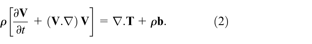
Equation (2) examines the temporal evolution of the velocity field

Here, the stress tensor is

Equation (4) expresses the extra stress tensor

Equation (5) provides a constitutive connection for the extra stress tensor in complex non-Newtonian Sisko fluids, involving material constants

Geometry of (a) lifting case (b) drainage case.
Model for the lifting case
Under the assumptions of thin film lubrication, the velocity vector is initially along the
The momentum equations reduce to:
By inserting the above formulations from equations (3) and (4) into equation (2), we derive:

The momentum balancing equation (2) is used to obtain equation (6), replacing stress tensor and velocity formulations, implying a constant pressure along the

The left side of the equation includes a nonlinear term involving the power
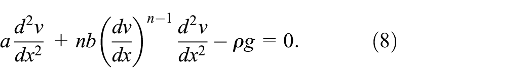
The equation incorporates gravity element

This outlines the problem’s boundary conditions. The velocity
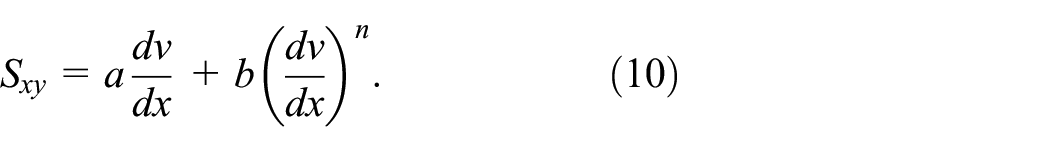
The standard linear shear stress is represented by the first component,

The equation indicates a zero-velocity gradient

The simplified momentum equation combines velocity derivatives with velocity gradient, gravity force per unit area, and a constant, incorporating linear and nonlinear shear stresses, and accounts for the effects on the velocity profile. Substituting
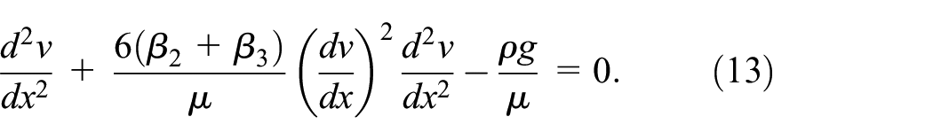
The equation (12) simplifies to include specific parameters like

Here,
The problem’s boundary conditions are determined by the velocity gradient at
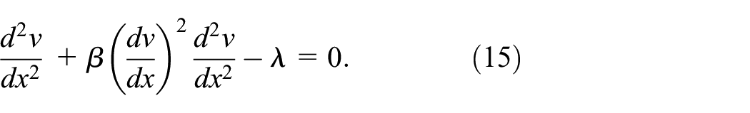
This equation is the dimensionless form of equation (13), obtained by introducing dimensionless parameters. The dimensionless parameter
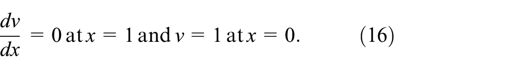
The boundary conditions for the dimensionless problem are

Equation (17) is a dimensionless form with a non-integer order derivative

The formulation’s boundary conditions for fractional calculus define the derivative of velocity as zero at
Model for the drainage case
Gravity plays a crucial role in fluid flow, particularly in thin film drainage flow. Gravity accelerates the fluid along the surface, facilitating its downward movement. The gravity-related pressure gradient, a spatial variation of pressure in the fluid, determines the direction and magnitude of fluid flow. In the case of drainage flow, this gradient resists the fluid’s downward motion due to pressure accumulation at the base of the film or the lower parts of the surface.
Equation (15), which originally models thin film flow dynamics with factors like viscosity and pressure gradients, will change when gravity is involved in drainage. The gravitational term and pressure gradient term need to be balanced in the governing equation, accounting for gravity-induced downward motion and the pressure gradient. Thus, gravity facilitates the flow by pulling the fluid downward, but the pressure gradient caused by the fluid’s weight pushes back, affecting the overall flow dynamics.

with
The formulation’s boundary conditions for fractional calculus define the derivative of velocity as zero at
General framework of Galerkin’s finite element
The following is the procedure used to formulate Galerkin’s finite element procedure, working from the governing differential equation to the matrix formulation:
I.Convert to standard form: The procedure starts with shifting the governing differential equation to the following form:

where
II.Use Quasi-linearization to address the governing equation’s nonlinearity: To transform the governing equation into a linear form, this method requires approximating the nonlinear variables.

The updated solution from the subsequent iteration is shown above as
III.Reduce to a linearized form: To make the equation simpler, the terms about

where
IV.Create the residual weighted form: The governing equation is linearized and then translated into a weighted residual form. This phase introduces the weighting function

Here,
V.Transform the weighted residual form into a weak form: To do this, the order of the derivatives is lowered by integrating parts (particularly for the second-order derivative

The boundary term
VI.Split the weak form equation into discrete parts: The weak form equation for the domain
VII. Approximate functions using a finite basis: The solution

where
VIII.Apply Galerkin’s finite element approach: It requires the weighting function

Substituting these approximations into the weak form results in a discretized system of equations.
IX.Formulate the equation system in matrix notation: A matrix representation of the discretized system of equations is provided. This results in a force vector and a stiffness matrix. The boundary term

This completes Galerkin’s finite element framework resulting in a system of linear equations that can be solved for the unknown nodal values
Galerkin’s finite element application to non-Newtonian third-grade Sisko fluid flow
It is necessary to select an appropriate trial or basis function that is applied locally across a typical finite element in the entire domain to use Galerkin’s finite element formulation44,55 in the finite element environment. We will use

The convention employed by Stasa
44
and Zienkiewicz
45
is to recast the above linear trial function in terms of values of the dependent functions at nodes

The nodal values of the dependent variable
Dynamics in lifting case
Considering the lifting case:

with
Our systematic methodology will be used to apply quasi-linearization 46 to the given nonlinear differential equation. Quasi-linearization is used to replace nonlinear differential equations with linear ones. We employ an iterative process, where:

The solution’s current approximation is denoted as

A common use of the quasi-linearization strategy is to represent the differential equations’ nonlinear part in terms of linear approximations centered on the current estimate,
Substitute the partial derivatives from (24) into (25) we get:

Now substituting
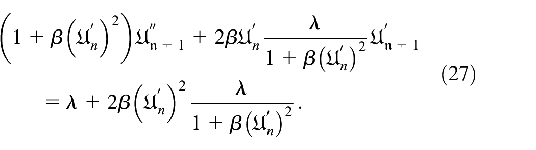

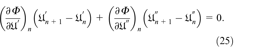
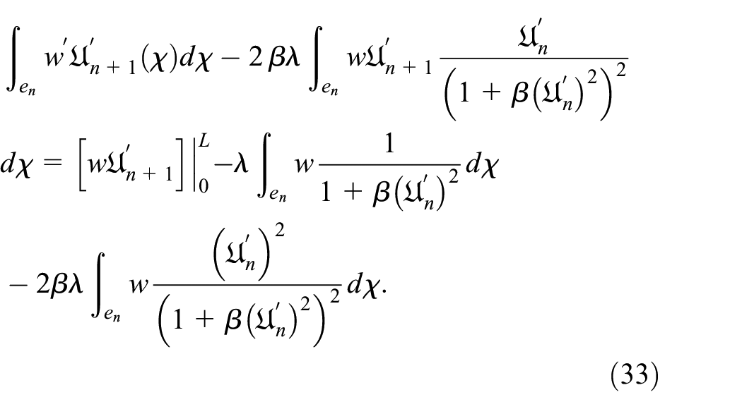
Equation (27) leads to the final linearized form presented in equation (28). For numerical techniques such as finite element formulation, a differential equation can be transformed into its weak form using the weighted residual approach. Here, we’ll obtain the weak formulation of the linearized differential equation by applying the weighted residual technique to it. The differential equation’s residual is denoted by

The residual


Taking the integration by parts of the first term of equation (31), and then rearranging, we will get:

This is the differential equation’s weak form. It is appropriate for use with finite element methods or other numerical approaches because it only requires the test function
Approximate
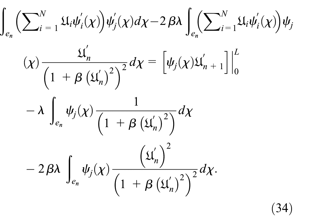
Two nodal values for a particular element are given by:
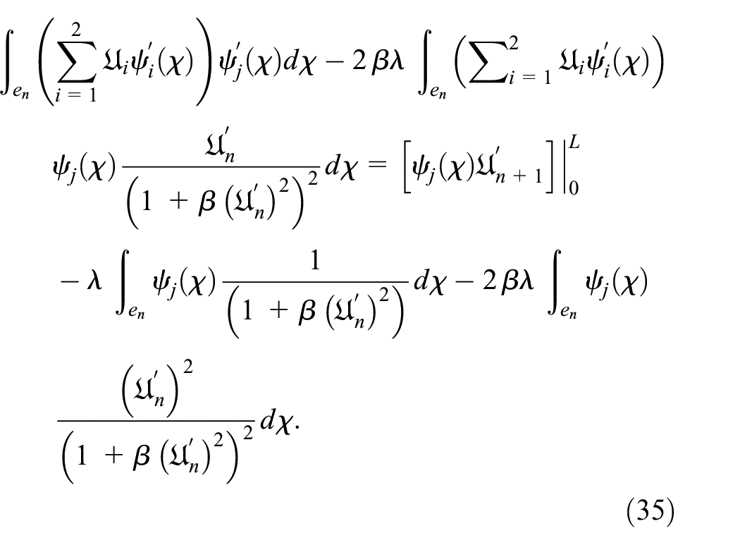
We can express the above equation in matrix form by collecting terms for each

Stiffness Matrix

Force Vector

Force Vector
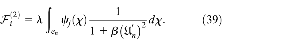
Force Vector

The global system of equations is assembled by summing contributions from each element over all elements

where

This matrix equation can then be solved for the unknown nodal values of
Dynamics in drainage case
When the fluid falls under gravity, the pressure gradient acts in the opposite direction, balancing the system to some extent. This means that the pressure gradient does not assist the flow but opposes it, potentially slowing the flow rate depending on the fluid’s thickness, viscosity, and surface slope. The governing equation (19) for the drainage changes to the following equation (43).

with
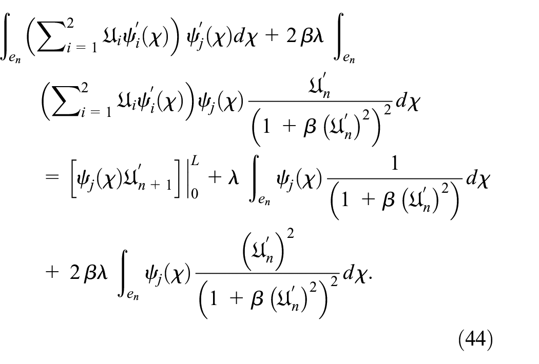
Following the calculations presented in Subsection “Dynamics in lifting case” we obtain the following relation for a particular element in the drainage case:
The global system of equations for the drainage case is assembled by summing over all elements similar to the lifting case.
Results and discussions
This article examines the behavior of third-grade non-Newtonian Sisko fluids (NNFs) in thin film under lifting and draining conditions using the finite element method (FEM). The outcomes for various values of the relevant parameters, together with residual errors to prove convergence are shown in Figures 2–13.

Impact of variations

Impact of variation in

Impact of simultaneous variations of

Impact of

Impact of

Mean absolute residuals

Impact of variations

Impact of variation in

Impact of simultaneous variations of

Impact of

Impact of

Mean absolute residuals
Figure 2 displays how the parameter
The gravitational parameter λ quantifies the relative strength of gravitational forces compared to viscous forces in the system. Figure 3 shows that the increasing value of λ (stronger gravity) opposes the lifting motion, causing the fluid velocity
The effects of several variations of parameters
Graph in Figure 5 demonstrates how the value of shear-thickening/ thinning parameter
The graph in Figure 6 indicates that the gravitational parameter
The mean absolute residuals
Figure 8 depicts the impact of the resistance generated by nonlinearity shear parameter β on the velocity of the Sisko fluid in drainage case. The slowest increasing curve indicates that the fluid’s characteristics change more gradually for decreasing levels of
The fluid’s behavior in this third-grade fluid drainage model is greatly influenced by the gravitational parameter
Figure 10 shows how the drainage behavior of a third-grade fluid is affected by various combinations of β and
For a drainage situation, when
In conclusion, the curve becomes less steep and the initial value of
Figure 12 shows the evolution of
In conclusion, greater values of
Figure 13 displays the logarithmic scale mean absolute residuals
The solution reported by Siddiqui et al. 7 using HPM for drainage cases is:

Table 1 presents the comparisons of absolute residual
Comparison of FEM absolute residuals with previous work for drainage case.

Source: aSiddiqui et al. 7
Significance and novelty of the current study
This work presented a finite element method-based framework for modeling both the lifting and drainage cases of thin-film third-grade non-Newtonian Sisko fluid flows, contributing a more accurate and robust solution method compared to previously published studies. Although several analytical and approximate methods have been used to study thin film flows of non-Newtonian fluids, a comprehensive Galerkin’s FEM analysis for third-grade and Sisko fluids in both lifting and drainage configurations has not been previously reported. The rationale behind opting Galerkin’s FEM is that Galerkin’s FEM has earned a great reputation in computational mechanics by meticulously uniting mathematical sophistication with practical robustness. It delivers high accuracy for nonlinear systems by minimizing error in a variational framework, supporting adaptive refinement, and preserving physics through weak-form conservation—outperforming alternatives like finite differences that lack these foundational advantages. Therefore, the novelty of the current work lies in the fact that, to the best of the authors’ knowledge, this is the first-ever application of Galerkin’s FEM framework to analyze both the lifting and drainage cases of thin-film third-grade non-Newtonian Sisko fluid flows. The proposed finite element method expands its strength over other numerical and semi-analytical methods in following notably important ways.
Unlike FDM, which require structured grid points and struggles when geometries are irregular, FEM uses flexible meshing due to which it is much more adaptive to complex domains.
Perturbation-based techniques (like HPM, HAM) have limited generality due to their heavily dependence on well-defined and small algorithmic parameters. In contrast, FEM is capable of handling high nonlinearities without necessitating such assumptions.
FEM permits the use of higher-order polynomial shape functions that leads to obtaining solutions with higher precision as compared to many low-order traditional schemes.
The governing equations for third-grade Sisko fluids are highly nonlinear. Complex boundary conditions are accurately handled without relying on small-parameter approximations. The local discretization and quasi-linearization techniques in FEM’s, ensure its stability and reliability in such nonlinear problems.
Since Sisko fluids contain intricate interactions between gravity and viscous forces, the authors were inspired to develop a framework that goes beyond a conventional solver. The authors wanted quantifiable endorsement of the obtained solutions strongly supported through residual error analysis. The results presented in this work demonstrate that FEM accomplishes residuals as low as
Conclusions
This work demonstrated the successful application of the finite element method (FEM) for examining thin film flows of non-Newtonian third-grade fluids regarding lifting and draining scenarios. The study depicts intricate fluid dynamics, even with intrinsic nonlinearities, employing a Galerkin-based FEM technique. The findings demonstrate FEM’s ability to efficiently predict velocity profiles and flow properties of the fluid, particularly how gravitational and material parameters influence these variables. In the lifting scenario, gravitational force affects velocity inversely, whereas the material parameter raises it to counterbalance gravitational attraction. In drainage scenarios, gravity enhances the flow rate while the material constant reduces it. Residuals remain very low in both scenarios confirming the accuracy, superior stability and precision of FEM’s over traditional methods. The methodology emphasizes FEM’s strengths in third-grade fluid studies, making it a useful tool in subsequent engineering and industrial applications. As a future direction, we aim to apply the same approach to more complex fractional models.
Footnotes
Appendix
Handling Editor: Sharmili Pandian
Funding
The author(s) received no financial support for the research, authorship, and/or publication of this article.
Declaration of conflicting interests
The author(s) declared no potential conflicts of interest with respect to the research, authorship, and/or publication of this article.
Data availability statement
All data generated or analyzed during this study are included in this manuscript.