Sage Journals: Discover world-class research

Abstract

Slender tubes are serving as crucial components for facilitating the reliable transport of gases and liquids in precision equipment across medical, aviation, and aerospace industries. The smoothness of their inner surfaces improved by reduced surface roughness is essential for ensuring the safe and efficient operation of such equipment. This study delved into the grinding mechanism of composite magnetorheological fluid and developed a material removal rate (MRR) model to identify key grinding process parameters. The influence of these parameters and their interactions on MRR and surface roughness (Sq) was studied, subsequently, the regression model constructed accordingly can predict machining performance. Notably, the optimal parameter combinations for maximizing MRR and minimizing surface roughness were found to be inconsistent. To reconcile this conflict, grey relational analysis (GRA) was applied to transform the multi-objective optimization problem into a single-objective optimization of grey relational grade (GRG), thereby enabling a comprehensive evaluation of grinding performance. A high quality surface with surface roughness Sq of 3.161 μm can be achieved at an material removal rate of 0.0610 μm/min under the condition of the optimized process parameters from grey correlation analysis. Compared with the results obtained by intuitive analysis, using this approach, the comprehensive grinding performance was improved by 42.71% and 32.74%, respectively. This study shows that the grinding process parameters of metal slender tube can be optimized by combinating of orthogonal test and grey correlation analysis, and which provides a new idea for the grinding of metal slender tube.

Keywords

orthogonal experiment grey relational analysis process parameter optimization material removal rate surface roughness

Introduction

Slender tubes are serving as crucial components for the transport of gases and liquids in some fields such as medicine, aviation, and aerospace, therefore, it is of great significance to improve the smoothness of the inner surface of the slender tube, that is, to reduce the roughness of the inner surface of the slender tube.^1–3 While the mechanical machining remains a cornerstone of modern manufacturing,⁴ it is ill-suited for processing slender tubes. The common grinding methods of inner surface of slender tubes are chemical grinding,^5–7 abrasive water jet grinding,^8–12 magnetic grinding,^13,14 and various other grinding methods.^15–18 However, each of these methods has its own limitations. Bi¹⁹ of Harbin Institute of Technology explored the process and mechanism of ion polishing of TC4 titanium alloy. The average surface roughness Ra can be reduced to less than 60 nm, and a good grinding effect has been obtained. Xiao et al.²⁰ machined a workpiece made from TC11 titanium alloy in composite magnetorheological fluid to address the issue of poor surface quality, and the optimal process parameters were obtained by orthogonal experiment, which greatly reduced the surface roughness of TC11 titanium alloy. Wu and Shi²¹ of Zhongyuan Institute of Technology used magnetic abrasive to grind T8A tool steel with Φ 20 mm diameter and 30 mm length under the condition of magnetic induction intensity of 0.3 T, and finally obtained the inner surface with surface roughness of 0.65 μm. Meng²² from Dalian University of Technology conducted magnetic grinding experiments on a 316L stainless steel tube with an outer diameter of 32 mm and an inner diameter of 28 mm, achieving a surface roughness of 0.18 μm. In 2011, Huang²³ used composite magnetic materials to process YL12 aluminum alloy tube with inner diameter of 32 mm and length of 40 mm under the condition of magnetic induction strength of 0.7 T, obtaining a wall roughness of 0.416 μm. The above researches reveal that while magnetic grinding can process high-quality inner surfaces, the tubes processed typically featured large diameters and low length-to-diameter ratios. Moreover, evaluations often relied solely on surface roughness (Sq), neglecting material removal rate (MRR), a critical factor in grinding efficiency. These can also indicate that grinding is a complex process involving multiple parameters and their interaction. But the effects of various process parameters on the grinding performance of slender tubes are mostly studied by single factor experiments without considering the interaction between parameters, making it difficult to comprehensively reveal the impact of these parameters on the grinding performance. Thus, innovative machining methods and multi-objective evaluation indicators are needed for processing slender tubes, in addition, when conducting multiple process parameter experiments, the experimental methods need to be carefully selected and designed. Composite magnetorheological fluids, a suspension in which the micron-sized magnetic particles are uniformly dispersed, which enables micro-cutting, friction, and sliding on the workpiece surface under the control of magnetic field. Because of its strong processing flexibility,^24–26 it is very suitable for processing slender tubes. The grinding process parameters play a crucial role in determining the surface quality of slender tube in the grinding process using composite magnetorheological fluids, directly affecting its functional performance, so the choice and optimization of grinding process parameters is quite important. Building upon our earlier work on shear stress modeling,²⁷ constructing an innovative material removal rate (MRR) model based on this shear stress, according to this model, key grinding process parameters can be identified.

Orthogonal design allows for fewer experiments while comprehensively analyzing the impact of parameters and their interactions on outcomes, distinguishing significant from insignificant parameters to achieve optimal parameter combinations. Grey relational analysis has clear advantages over orthogonal design in solving multi-criteria optimization problems. This method has been successfully applied in various engineering fields, such as laser processing, mechanical design, and ultra-precision milling and grinding and so on. Senthilkumar et al.²⁸ optimized the mixing of transformer oil and natural ester oil using orthogonal experiments and grey relational analysis. Kursuncu and Biyik²⁹ also utilized these methods to optimize cutting parameters of AISIO2 steel, demonstrating that combining orthogonal experiments with grey relational analysis is superior to using either method alone when addressing optimization problems involving multiple parameters and criteria. Therefore, orthogonal experiment is used to systematically investigate the influences of process parameters on material removal rate (MRR) and surface roughness (Sq), the multi-criteria optimization challenge is transformed into a single-objective optimization evaluation by using grey relational analysis method, thereby offering an innovative methodology for precision grinding of slender tubes.

Theoretical analysis

The grinding of workpiece using composite magnetorheological fluid relies predominantly on tangential shear forces. Schematic diagram of magnetic chain shear action is shown in the Figure 1(a), while Figure 1(b) provides a magnified view of the micro-cutting action of a composite magnetic particle in intimate contact with the workpiece surface. Let point O denote the centroid of a composite magnetic particle, where $τ$ represents the shear stress of the magnetic chain acting on the composite magnetic particle, and $B$ signifies the magnetic induction intensity. When relative motion occurs between the composite magnetic particle and the workpiece surface, the shear stress will resists this motion, the greater the shear stress, the stronger the shear action of composite magnetic particles on the workpiece surface.

Figure 1.

Grinding schematic diagram of composite magnetic particles: (a) schematic diagram of magnetic chain shear action and (b) a magnified view of the micro-cutting action of a composite magnetic particle.

Under research,²⁷ the shear stress generated by the magnetic chain can be calculated as shown in equation (1).

τ = \frac{2 A ϕ R^{3} B^{2} χ^{2}}{3 μ_{0} {(1 + χ_{1})}^{2} {(2 R + 2 t + δ)}^{3}} ξ

(1)

In the equation, A is the model size coefficient, $ϕ$ is volume fraction of magnetic particles in the composite magnetorheological fluids, $R$ is radius of magnetic particles, $B$ is magnetic induction intensity, $χ$ is magnetic susceptibility of magnetic particles, $μ_{0}$ is vacuum permeability, $χ_{1}$ is magnetic susceptibility of composite magnetorheological fluids, $t$ is coating thickness of abrasive grain, $δ$ is interparticle distance between magnetic particles, $ξ$ is shear stress coefficient of composite magnetorheological fluids.

To achieve uniformity of composite magnetorheological fluid grinding, it is essential to ensure that the composite magnetorheological fluid has both rotational motion and horizontal linear motion relative to the slender tube. The schematic diagram of motion of single composite magnetic particles relative to the slender tube is presented in Figure 2.

Figure 2.

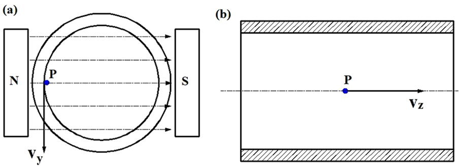
Motion of composite magnetic particle relative to the slender tube during grinding: (a) the motion in the y-direction and (b) the motion in the z-direction.

As known from Figure 2(a) and (b), the velocity of circumferential motion of the slender tube is $v_{y}$ , while the velocity of axial motion of the magnetic pole is $v_{z}$ . The $v_{y}$ can be calculated using the following equation:

v_{y} = w R_{in} = 2 π n_{t} R_{in}

(2)

In the equation, $w$ represents the rotational angular velocity of the slender tube (rad/s), $n_{t}$ is the rotational speed of the slender tube (r/s), and $R_{in}$ is the inner radius of the slender tube.

Considering the hysteresis of composite magnetic abrasive particles, the relationship between the circumferential velocity $v_{y 1}$ of composite magnetic abrasive particles relative to the slender tube and the circumferential velocity $v_{y}$ of the slender tube is shown in equation (3).³⁰

v_{y 1} = \frac{1}{6} v_{y}

(3)

Equation (4) can be derived from equations (2) and (3), as shown below.

v_{y 1} = \frac{1}{3} π n_{t} R_{in}

(4)

The movement of a composite magnetorheological fluid within the slender tube is quite complex. In order to simplify the analysis, it is assumed that the motion of the composite magnetorheological fluid within the slender tube was in the best state, that is, the axial velocity $v_{z 1}$ of the composite magnetic particles relative to the slender tube is equal to the axial feed velocity $v_{z}$ of the magnetic pole.³¹ Considering the hysteresis of composite magnetic abrasive particles, the following equation can be obtained.

v_{z 1} = \frac{1}{6} v_{z}

(5)

From equations (4) and (5), the resultant velocity $V_{r}$ of the relative motion between the composite magnetic particles and the slender tube was expressed as equation (6).

V_{r} = \sqrt{v_{y 1}^{2} + v_{z 1}^{2}} = \frac{1}{3} \sqrt{π^{2} n_{t}^{2} R_{in}^{2} + \frac{1}{4} v_{z}^{2}}

(6)

The Preston equation is a material removal model used in the field of optical polishing, and the grinding of the slender tube with the composite magnetorheological fluid can be described by the removal model,³² which is expressed as follows.

MRR = K_{τ} τ V_{r}

(7)

In the equation, $MRR$ represents the material removal rate (μm/s), $K_{τ}$ is the Preston coefficient of shear load, $τ$ is the shear stress of the composite magnetorheological fluids, and $V_{r}$ is the relative motion velocity between the composite magnetorheological fluid and the slender tube (m/s).

Equation (8) can be obtained by substituting the shear stress calculation equation for composite magnetorheological fluid from the equations (1) and (6) into equation (7).

MRR = K_{τ} \frac{2 A ϕ R^{3} B^{2} χ^{2} ξ}{9 μ_{0} {(1 + χ_{1})}^{2} {(2 R + 2 t + δ)}^{3}} \sqrt{π^{2} n_{t}^{2} R_{in}^{2} + \frac{1}{4} v_{z}^{2}}

(8)

In the equation, $n_{t}$ is the rotational velocity of the slender tube, and $v_{z}$ is the axial motion velocity of the magnetic pole.

As revealed in equation (8), the material removal rate (MRR) of the composite magnetorheological fluid is relevant to the magnetic induction intensity $B$ , the rotational speed $n_{t}$ of the slender tube, and the movement speed $v_{z}$ of the magnetic pole, in addition to intrinsic properties of magnetic particles. Therefore, the magnetic induction intensity, the rotational speed of the slender tube, and the moving speed of the magnetic pole are selected as the process parameters for studying the grinding effectiveness on the slender tube inner wall.

The fundamental mechanism of composite magnetorheological fluid grinding involves the micro-cutting, rolling, and sliding effects exerted by composite magnetic abrasive particles on the workpiece surface, achieving material removal and reducing surface roughness. Thus, the study evaluates grinding performance using material removal rate and surface roughness as primary indicators.

Experiment

Experimental setup

A CY6140 lathe was selected as the main grinding equipment that provides power. The grinding device of composite magnetorheological fluid is shown in Figure 3. When grinding, one end of the slender tube was sealed with a cap, and the prepared composite magnetorheological fluid was injected into the slender tube with a syringe, and then the sealed end was clamped on the spindle of the machine tool to achieve a relative rotational motion of the composite magnetorheological fluids. The NdFeB magnetic strip (length × width × thickness is 90 mm × 10 mm × 6 mm) held in place by a self-developed support blocks was fixed on the slide box of the CY6140 ordinary lathe through the magnetic meter base to realize the relative horizontal movement of the composite magnetorheological fluids. This setup ultimately enabled the resultant motion of the composite magnetorheological fluids, ensuring the grinding uniformity.

Figure 3.

A grinding device of composite magnetorheological fluids: (a) schematic diagram of the grinding device and (b) schematic diagram of the grinding principle.

Experimental design

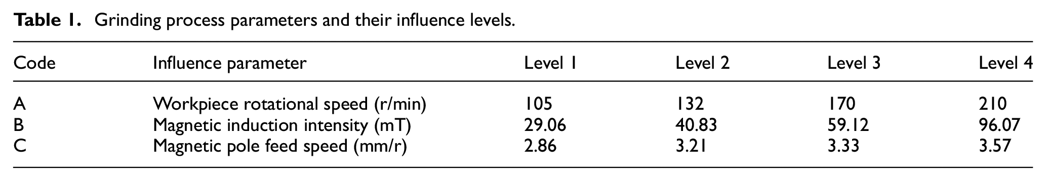
According to the material removal rate model of shear stress, the main process parameters affecting MRR are workpiece speed $n_{t}$ , magnetic induction intensity $B$ , and feed speed $v_{z}$ of magnetic pole under the premise of prepared composite magnetorheological fluid with better performance. After consulting the relevant literature, it is concluded that the relatively low workpiece speed and magnetic pole feed speed have favorable effects on the material removal rate and surface roughness. In addition, since the CY6140 conventional lathe was selected as the main machine for grinding experiments, the lathe spindle speeds meeting the mentioned requirements were 105, 132, 170, and 210 r/min, and the corresponding feed speeds were 2.86, 3.21, 3.33, and 3.57 mm/r. The magnetic induction intensity was adjusted by controlling the distance between the magnetic stripe and the workpiece, ensuring that the closest distance from single magnetic stripe to workpiece was 1 mm. The single magnetic stripe was then moved outward by 2, 1, and 1 mm, respectively. As a result, the magnetic induction densities measured at various distances from nearest to farthest, were 96.07, 59.12, 40.83, and 29.06 mT. Therefore, the experimental parameters (the Magnetic induction intensity $B$ , the workpiece rotational speed $n_{t}$ , and the magnetic pole feed speed $v_{z}$ ) and their influence levels were set as shown in Table 1. This experiment was designed using a 3-factor and 4-level orthogonal array.

Table 1.

Grinding process parameters and their influence levels.

Code	Influence parameter	Level 1	Level 2	Level 3	Level 4
A	Workpiece rotational speed (r/min)	105	132	170	210
B	Magnetic induction intensity (mT)	29.06	40.83	59.12	96.07
C	Magnetic pole feed speed (mm/r)	2.86	3.21	3.33	3.57

Experimental characterization

Material removal rate

The grinding efficiency of the composite magnetorheological fluid on the slender tube was measured by the MRR, that is, the material removal rate is measured by the thickness of material removed per unit time (the quality of slender tube before and after grinding is measured by FA2004N precision electronic analysis balance with precision of 0.1 mg). The equation is as follows.

MRR = (\sqrt{\frac{Δ m}{ρ_{s} π l} + R_{s}^{2}} - R_{s}) / t_{1}

(9)

In the equation, $MRR$ represents the material removal rate (μm/s), $Δ m$ is the change in mass of the slender tube before and after grinding, $ρ_{s}$ is the density of the material, $l$ is the processed length of the slender tube, $R_{s}$ is the radius of the slender tube before grinding, and $t_{1}$ is the grinding time of the composite magnetorheological fluid on the slender tube.

Surface roughness

Three-dimensional morphology of the workpiece surface was analyzed by a three-dimensional root-mean-square deviation $S_{q}$ , the roughness of the grinded surface of the slender tube was characterized by using an LI-3 contact surface profilometer. Then, the morphology of the grinded surface of the workpiece was observed by using a high-resolution field emission scanning electron microscope (FESEM).

Results and analysis

The experimental results of the effects of process parameters on material removal rate (MRR) and surface roughness (Sq) were shown in Table 2. Multivariate regression analysis, analysis of variance (ANOVA), and grey relational analysis were performed based on the experimental results. It can be seen from Table 2 that the grinding efficiency of the composite magnetorheological fluid was the highest, which is 0.0598 μm/min when the rotational speed of the workpiece was 132 r/min, the magnetic induction intensity was 96.07 mT, and the magnetic pole feed speed was 3.33 mm/r; the smallest surface roughness was obtained, which was 3.158 μm when the workpiece speed is 105 r/min, the magnetic induction intensity is 59.12 mT, and the magnetic pole feed speed is 3.33 mm/r. The parameter combinations that produce maximum material removal rate (MRR) and minimum surface roughness (Sq) are inherently conflicting, necessitating alternative analytical methods to optimize the experimental results.

Table 2.

Results of MRR and Sq obtained in the L16(4³) orthogonal experiment.

Sample	Workpiece rotationalspeed (r/min)	Magnetic inductionintensity (mT)	Feed speed(mm/r)	Material removalrate (μm/min)	Surface roughness(μm)
1#	105	29.06	2.86	0.0301	3.391
2#	105	40.83	3.21	0.0332	3.472
3#	105	59.12	3.33	0.0451	3.158
4#	105	96.07	3.57	0.0513	3.265
5#	132	29.06	3.21	0.0317	3.541
6#	132	40.83	2.86	0.0378	3.214
7#	132	59.12	3.57	0.0416	3.311
8#	132	96.07	3.33	0.0598	3.164
9#	170	29.06	3.33	0.0179	3.713
10#	170	40.83	3.57	0.0247	3.386
11#	170	59.12	2.86	0.0406	3.215
12#	170	96.07	3.21	0.0465	3.402
13#	210	29.06	3.57	0.0112	3.815
14#	210	40.83	3.33	0.0198	3.576
15#	210	59.12	3.21	0.0308	3.533
16#	210	96.07	2.86	0.0432	3.614

Surface morphology analysis

The grinded surface morphologies of the slender tube with the composite magnetorheological fluid were illustrated in Figure 4. As observed in Figure 4(c) and (m), sample 3 exhibits the minimum surface roughness Sq, which is 3.158 μm, while Sample 13 shows the maximum surface roughness Sq, which is 3.815 μm. It can also be seen that the fluctuation ranges of the surface roughness of the samples 3 and 6 with smaller surface roughness are smaller, which fluctuate in the range of −16 to 12 μm, especially that of the sample 3 fluctuates in the range of −8.54 to 11.529 μm, while those of the samples 2, 5, and 16 with larger surface roughness fluctuate in the range of −11 to 39.3 μm. It can be seen From Table 2 that sample 3 achieved a roughness of 3.158 μm, indicating the best surface quality when the rotational speed of the slender tube is 105 r/min, the magnetic induction intensity is 59.12 mT, and the magnetic pole feed speed is 3.33 mm/r; when the rotational speed of workpiece is 210 r/min, the Magnetic induction intensity is 29.06 mT, and the magnetic pole feed speed is 3.57 mm/r, Sample 13 resulted in a roughness of 3.815 μm, representing the worst surface quality. The above analysis indicates that elevated magnetic induction intensity substantially decreases workpiece surface roughness (Sq) while enhancing surface finish quality, because the enhanced magnetic induction intensity operates through three synergistic mechanisms: first, a increase in MR fluid viscosity; second, shear stress (τ) amplification; and third, formation of reinforced magnetic chains. These microstructural changes collectively account for the reduced surface roughness, as shown in Figure 1(a), a reduced $θ$ value is simultaneously formed under these conditions.

Figure 4.

Microscopic morphologies of samples after magnetic grinding: (a) sample 1, (b) sample 2, (c) sample 3, (d) sample 4,(e) sample 5, (f) sample 6, (g) sample 7, (h) sample 8, (i) sample 9, (j) sample 10, (k) sample 11, (l) sample 12, (m) sample 13,(n) sample 14, (o) sample 15, and (p) sample 16.

The surface profiles of the samples before and after grinding were measured by LI-3 contact surface profiler, and the results are shown in Figure 5. As can be seen from Figure 5, after 60 min of grinding with the composite magnetorheological fluids, the surface roughness Ra of the workpiece declined by 23.22% from 4.121 to 3.164 μm, and the average spacing between microscopic uneven areas in the profile was greatly reduced, indicating that the surface quality of the workpiece has been significantly improved after grinding with composite magnetorheological fluids. The surface morphologies of sample 8 before and after grinding are shown in Figure 6. It can be seen from Figure 6(a) and (b) that the surface morphology of the sample after magnetic grinding is flatter than that before grinding. Moreover, before magnetic grinding, there were large convex areas as well as dense, large, and deep concaves on the workpiece surface. Therefore, the average spacing between microscopic uneven areas in the profile was large before grinding. However, after magnetic grinding, convex areas on the workpiece surface were smaller than those before the grinding, as quantitatively demonstrated in Figure 1(b), this topographical modification results from the shearing action of composite magnetic particles on workpiece protrusions during the grinding process. Thereby, the average spacing between microscopic uneven areas in the profile was small after grinding.

Figure 5.

The material removal profile curves for sample 8: (a) sample 8 before grinding and (b) sample 8 after grinding.

Figure 6.

Surface morphologies of sample 8 before and after grinding: (a) sample 8 before grinding and (b) sample 8 after grinding.

Multivariate regression analysis and ANOVA for MRR and Sq

The results of the multiple regression analysis and regression variance analysis of the MRR and Sq were shown in Table 2, and the multiple regression models between MRR and Sq and the parameters were constructed as shown in equations (10) and (11). The results of regression equation variance analysis were shown in Tables 3 and 4, and the comparative results of regression equation predicted values and measured values were shown in Figures 7 and 8.

\begin{matrix} MRR = 0.0637 - 0.000263 A + 0.000921 B - 0.013 C \\ - 0.000004 B^{2} + 0.000035 A * C \end{matrix}

(10)

\begin{matrix} S_{q} = 3.476 + 0.00006 A - 0.04116 B + 0.265 C \\ + 0.000224 B^{2} + 0.000061 A * B \end{matrix}

(11)

Table 3.

ANOVA for the regression model of MRR.

Source	Degree offreedom	Sum of squared deviations from the mean	Mean square	F_MRR	P_MRR	Significance
A	1	0.000004	0.000004	0.33	0.577
B	1	0.000140	0.000140	10.48	0.009	***
C	1	0.000005	0.000005	0.35	0.568
B × B	1	0.000048	0.000048	3.58	0.088	*
A × C	1	0.000001	0.000001	0.06	0.810
Regression	5	0.002381	0.000476	35.53	0.000	***
Error	10	0.000134	0.000013
Total	15	0.002515
			R ² = 0.9467	R ² _adjusted = 0.9201

Note. p < 0.01 indicates a very significant effect and is denoted by ***; p < 0.05 indicates a relatively significant effect and is denoted by **; p < 0.1 indicates a generally significant effect and is denoted by *.

Table 4.

Variance analysis of the regression model for Sq.

Source	Degree offreedom	Sum of squareddeviations fromthe mean	Mean square	F_Sq	P_Sq	Significance
A	1	0.000007	0.000007	0.00	0.981
B	1	0.210955	0.210955	18.03	0.002	***
C	1	0.033923	0.033923	2.90	0.119
B × B	1	0.173546	0.173546	14.83	0.003	***
A × C	1	0.027561	0.027561	2.36	0.156
Regression	5	0.613593	0.122719	10.49	0.001	***
Error	10	0.117023	0.011702
Total	15	0.730616
			R² = 0.8398	R²_adjusted = 0.7597

Figure 7.

The comparison between the predicted and the measured of MRR: (a) the comparison between the predicted and the measured of MRR, (b) the relative error between the predicted and the measured of MRR.

Figure 8.

The comparison between the predicted and the measured of Sq: (a) the comparison between the predicted and the measured of Sq, (b) the relative error between the predicted and the measured of Sq.

As can be seen from Table 3, the correlation coefficient R² of regression model for MRR is 0.9467, and the adjusted correlation coefficient R² is 0.9201, indicating that the regression model for MRR can explain 92.01% of the variance in the response, demonstrating a good fit of the obtained regression model for MRR to predict the MRR. It can also be concluded from Table 3 that B × B is significant at the significant level below 0.1, and the Magnetic induction intensity B is remarkable at the significant level below 0.01, indicating marked influences of relevant factors and their interactions on MRR. It can be revealed from F_MRR that the order of importance of the parameters affecting the MRR was that magnetic induction intensity (B) is greater than magnetic pole feed speed (C), and magnetic pole feed speed (C) is greater than workpiece rotational speed (A), the F_MRR for magnetic induction intensity (B) is the largest, which is 10.48, indicating that magnetic induction intensity (B) has the most significant impact on the MRR, and elastic analysis of equation (8) establishes magnetic induction intensity as the predominant factor governing material removal rate (MRR). While the F_MRR for workpiece rotational speed (A) was the smallest, which is 0.33, indicating that workpiece rotational speed (A) had the weakest influence on MRR.

It can be seen from Table 4 that the correlation coefficient R² of the regression model for Sq was 0.8398, and the adjusted correlation coefficient R² is 0.7597, indicating that the regression model for Sq can explain 75.97% of the variance in the response, demonstrating a good fit of the obtained regression model for Sq to predict the Sq. It can also be concluded from Table 4 that the magnetic induction intensity (B) and B × B are significant at the significant level below 0.01, indicating marked influences of relevant factors and their interactions on Sq. It can be revealed from F_Sq that the order of importance of the parameters affecting the Sq was that magnetic induction intensity (B) is greater than magnetic pole feed speed (C), and magnetic pole feed speed (C) is greater than workpiece rotational speed (A). The F_Sq for Magnetic induction intensity (B) is the largest, which is 18.03, indicating that Magnetic induction intensity (B) has the most significant impact on the Sq. While the F_Sq for workpiece rotational speed (A) was the smallest, which is 0, indicating that workpiece rotational speed (A) had the weakest influence on MRR.

From the comparison between the predicted and the measured of MRR in Figure 7(a), it can be seen that the predicted is close to the measured, and the relative error is less than 19% (Figure 7(b)). It further shows that the regression model for MRR can predict MRR under various process parameters.

From the comparison between the predicted and the measured of Sq in Figure 8(a), it can be seen that the predicted is close to the measured, and the relative error is less than 5.5% (Figure 8(b)), showing that the regression model for Sq has high accuracy and can predict Sq under various process parameters.

The effect curve of MRR is shown in Figure 9. It can be seen that MRR first increases and then decreases with the increase of workpiece rotation speed. The reason is that the relative velocity between the composite magnetorheological fluid and the workpiece increases with the increase of workpiece rotation speed, thereby heightening the MRR.

Figure 9.

The effect curve of MRR.

While equation (8) satisfactorily validates this conclusion, excessive rotational speed of the workpiece disrupts the magnetic chain structures. The composite magnetic particles become dispersed and align with the flow direction, failing to reorganize into new chains even under magnetic field excitation. Consequently, the shear stress is significantly reduced, thus gradually reducing the MRR. In addition, MRR increases with the increase of magnetic induction intensity (B). The reason is that the higher the magnetic induction intensity is, the stronger the magnetorheological effect is, the larger the shear yield stress of the composite magnetorheological fluid is, and thereby the higher the MRR is. However, when the Magnetic induction intensity reaches a certain value, the MRR almost do not change. It was also found that the MRR decreases as the magnetic pole feed speed (C) increases. Finally, it can be seen that under the condition of A2B4C1, that is, when the rotational speed of the workpiece is 132 r/min, the magnetic induction intensity is 96.07 mT, and the magnetic pole feed speed is 2.86 mm/r, the MRR is the highest.

It can be seen from Figure 10 that the Sq increases with the increase of the rotational speed of the workpiece. The reason is that the greater the relative velocity is between the composite magnetorheological fluid and the workpiece with the increase of the rotational speed of the workpiece, as evidenced in Figure 1(b), the abbreviated interaction duration between individual magnetic particles and the workpiece surface prevents complete material removal, resulting in irregular micro-scale peak-valley topography formation, the larger roughness of the grinded surface is, so the surface roughness reaches the minimum at 105 r/min. The surface roughness of the workpiece decreases at first and then increases with the increase of magnetic induction intensity (B). The reason is that when the magnetic induction intensity increases, it can be analyzed from equation (1) that the shear stress of the composite magnetorheological fluid increases, enhancing the grinding capacity, so the surface roughness decreases, reflected in a improving trend in the surface quality of the workpiece. However, as the Magnetic induction intensity increases further, the composite magnetic particles are subjected to excessive magnetic pressure, thus scratching the workpiece surface. As a result, the surface roughness shows an increasing trend with the further increase of magnetic induction intensity. Therefore, the surface roughness was the minimum when the magnetic induction intensity was 59.12 mT. The surface roughness of the workpiece increases at first, then decreases and then increases with the increase of magnetic pole feed speed (C). As ultimately displayed, the surface roughness (Sq) reached the minimum under the conditions of A1B3C1, where the workpiece rotational speed was 105 r/min, the Magnetic induction intensity was 59.12 mT, and the magnetic pole feed speed was 2.86 mm/r. In other words, the surface quality achieved the best under this parameter combination.

Figure 10.

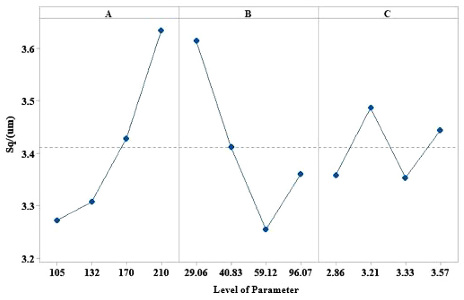
The effect curve of Sq.

Coordination between MRR and Sq

Based on the above analysis, we can conclude that the effects of rotational speed of workpiece (A), magnetic induction intensity (B), magnetic pole feed speed (C), and their interactions on MRR and Sq were different. Moreover, the effect curves indicated that the optimal process parameter combinations obtained under each evaluation index were also different, for instance, the maximum MRR (i.e. the highest grinding efficiency) was achieved under the condition of A2B4C1, while the minimum Sq (i.e. the best surface quality) was obtained under the condition of A1B3C1. The above two parameter combinations were not included in the orthogonal experiment. Therefore, it is still necessary to use other analysis methods to obtain the optimal process parameter combinations.

Grey relational analysis is a method suitable for assessing the correlation degree among multiple factors or evaluation indices, and has remarkable advantages in solving multi-index problems. Composite magnetorheological fluid grinding is an incomplete grey system formed by the interaction between process parameters and evaluation indexes, making it particularly suitable for grey relational analysis. Therefore, the grey correlation analysis method was used to solve the coordination between MRR and Sq.

Results of coordination between MRR and Sq

After processing the orthogonal test results in Table 2 using the grey relational analysis method, the ND, GRC, GRG, and the ranking of GRG were obtained as shown in Table 5. GRG is used to evaluate the comprehensive performance of MRR and Sq. The larger the GRG is, the better the corresponding experimental result is. The performance of each evaluation index MRR or Sq can be obtained from their effect curve analysis. Therefore, the complex multi-index optimization problem can be transformed into a single GRG optimization problem by using the grey relational analysis method. According to the values and rank of GRG shown in Table 5, the largest grey correlation degree (GRG) is 0.67194 under the condition of the parameters combination, which is that the rotational speed of workpiece is 132 r/min, the magnetic induction intensity is 96.07 mT, and the magnetic pole feed speed is 3.33 mm/r, so that, the larger MRR and smaller Sq can be obtained at the same time under this condition, the underlying mechanism can be attributed to synergistic effects among parameters. In composite magnetorheological fluid grinding, a higher magnetic induction intensity not only stabilizes the magnetic chain structures of magnetic particles but also generates greater shear stress. Consequently, even under high magnetic pole feed speed condition covering large processing areas, the magnetic abrasive particles maintain uniform distribution. This accounts for why this parameter combination achieves both higher material removal rate and lower surface roughness.

Table 5.

The ND, GRC, GRG, and the GRG Rank.

Exp. no.	MRR (j = 1)		Sq (j = 2)		GRG	Rank
Exp. no.	ND	GRC	ND	GRC	GRG	Rank
1	0.38889	0.45000	0.49707	0.44590	0.44795	14
2	0.45268	0.47741	0.40211	0.49868	0.48805	9
3	0.69753	0.62308	1.00000	0.28571	0.45440	13
4	0.82510	0.74085	0.64478	0.38285	0.56185	5
5	0.42181	0.46374	0.32122	0.55462	0.50918	7
6	0.54733	0.52484	0.70457	0.36213	0.44348	15
7	0.62551	0.57176	0.59086	0.40369	0.48773	10
8	1.00000	1.00000	0.76319	0.34388	0.67194	1
9	0.13786	0.36707	0.11958	0.76986	0.56846	4
10	0.27778	0.40909	0.50293	0.44300	0.42605	16
11	0.60494	0.55862	0.70340	0.36252	0.46057	12
12	0.72634	0.64628	0.48417	0.45240	0.54934	6
13	0.00000	0.33333	0.00000	1.00000	0.66667	2
14	0.17696	0.37792	0.28019	0.58807	0.48300	11
15	0.40329	0.45591	0.33060	0.54750	0.50170	8
16	0.65844	0.59413	0.23564	0.62929	0.61171	3

The results of range analysis, variance analysis, and effect curve analysis of GRG were displayed in Tables 6 and 7, as well as Figure 11. As revealed from the R_GRG and F_GRG in Tables 6 and 7, the order of importance of the parameters influencing the GRG was that magnetic induction intensity (B) is greater than workpiece rotational speed (A), and workpiece rotational speed (A) is greater than magnetic pole feed speed (C), it can be seen that the influence of magnetic induction intensity (B) is the most significant, it can be known that in the grinding of composite magnetorheological fluids, the magnetic induction intensity (B) is the dominant factor, because the magnetic induction intensity directly determines the rheological properties of the composite magnetorheological fluids. When magnetic induction intensity is increased, a magnetic chain structure with greater shear stress can be formed, laying the foundation for improving the grinding comprehensive performance.

Table 6.

Range analysis of GRG.

The average value	A	B	C
k_{GRG 1}	0.4881	0.5481	0.4909
k_{GRG 2}	0.5281	0.4601	0.5121
k_{GRG 3}	0.5011	0.4761	0.5444
k_{GRG 4}	0.5658	0.5987	0.5356
R_GRG	0.0777	0.1386	0.0535

Table 7.

Variance analysis of GRG.

Source	Degree offreedom	Sum of squareddeviations fromthe mean	Mean square	F_GRG	P_GRG	Significance
A	3	0.014140	0.004713	1.53	0.300
B	3	0.049964	0.016655	5.41	0.038	**
C	3	0.006985	0.002328	0.76	0.558
Error	6	0.018465	0.003078
Total	15	0.089553

Figure 11.

The effect curve of GRG.

As discovered from Figure 11, the GRG displayed a trend of first increase, then decrease, and finally increase again with the increase in the workpiece rotational speed (A), a trend of first decrease and then increase with the increment in the Magnetic induction intensity (B), and a trend of first rise and then drop with the increase in the magnetic pole feed speed. As unveiled through the effect curve analysis with multiple evaluation indices, the optimal combination of process parameters was A4B4C3, that is, there was the maximum GRG when the rotational speed of the workpiece was 210 r/min, the magnetic induction intensity was 96.07 mT, and the magnetic pole feed speed was 3.33 mm/r, indicating the best comprehensive performance of composite magnetorheological fluid grinding, but this parameters combination are not reflected in the orthogonal experiment, consequently, experimental validation will be performed to study the effects of this parameter combination on grinding performance.

Verification of the coordination between MRR and Sq

It can be seen that the optimal combinations (i.e. MRR (A2B4C1) and Sq (A1B3C1)) obtained from the effect curve analysis of single evaluation indices differed from those (i.e. A2B4C3 and A4B4C3) obtained through grey relational (GRG) analysis. To validate the effectiveness of the grey relational analysis method, the optimal combinations obtained by grey relational analysis and the optimal combinations obtained by effect curve analysis under single evaluation index were tested and compared. Further, the experimental results were predicted using the mentioned regression model with each single evaluation index. Verification of the experimental schemes and results was presented in Table 8, and the comparison between the predicted results and experimental results was shown in Table 9. The corresponding surface morphologies were shown in Figure 12.

Table 8.

Verification of the experimental schemes and results.

Evaluation index(parametercombination)	Processparameters			Experimentalresults
	Workpiecerotationalspeed (r/min)	Magneticinductionintensity(mT)	Feedspeed(mm/r)	MRR(μm/min)	Sq (μm)	GRG
MRR(A2B4C1)	132	96.07	2.86	0.0604	3.162	0.4722
Sq(A1B3C1)	105	59.12	2.86	0.0601	3.163	0.5077
GRG1(A2B4C3)	132	96.07	3.33	0.0598	3.164	0.6667
GRG2(A4B4C3)	210	96.07	3.33	0.0610	3.161	0.6739

Table 9.

The comparison between the predicted results and experimental results.

Evaluation index (parameter combination)	MRR (μm/min)predicted value	Relativeerror (%)	Sq (μm) predictedvalue	Relative error (%)
MRR(A2B4C1)	0.0566	−6.32	3.129	−1.06
Sq(A1B3C1)	0.0491	−18.29	3.093	−2.21
GRG1(A2B4C3)	0.0526	−11.97	3.253	2.82
GRG2(A4B4C3)	0.0489	−19.92	3.715	17.52

Figure 12.

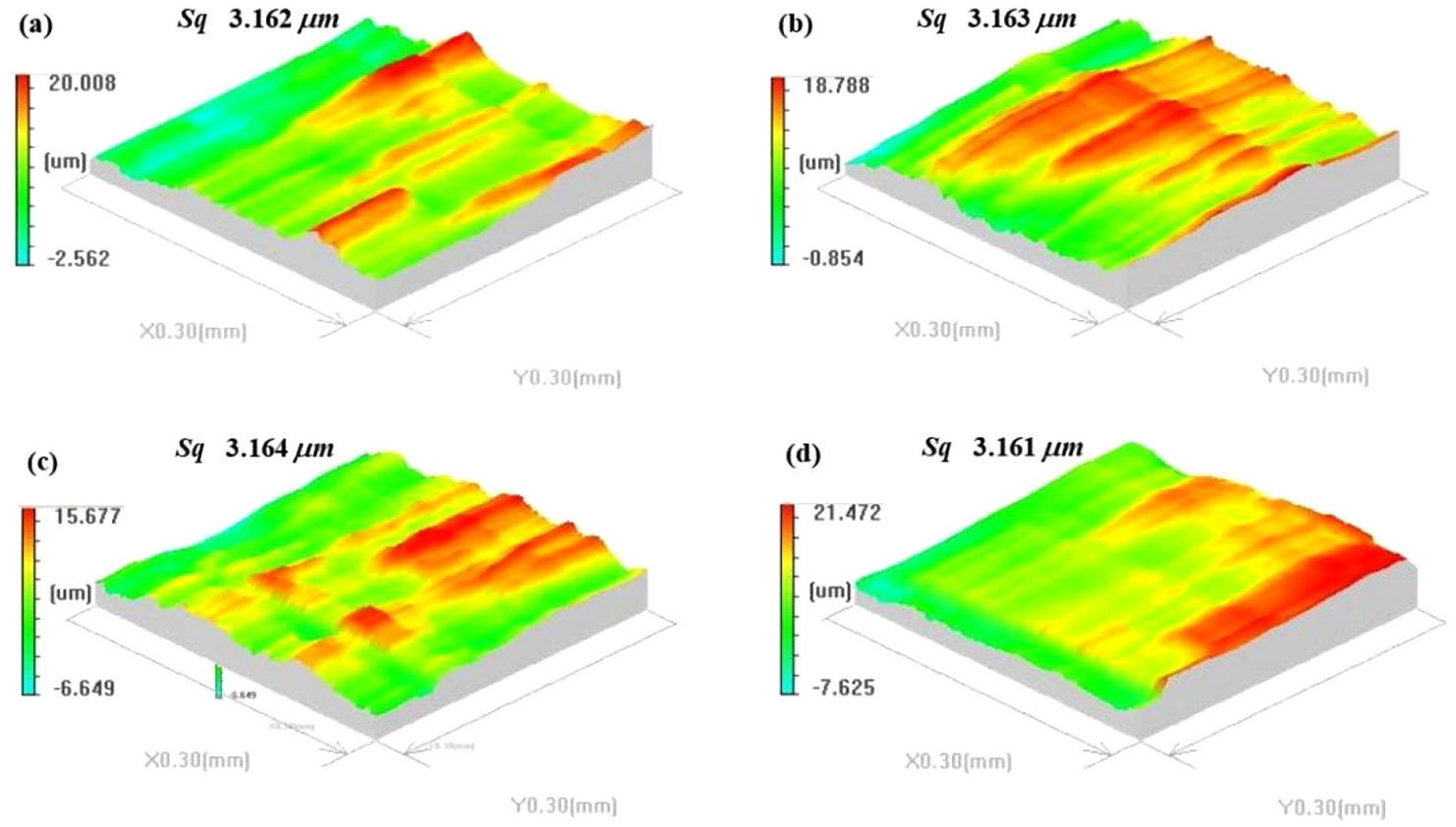
Surface morphologies obtained through optimal experimental combinations: (a) MRR (A2B4C1), (b) Sq (A1B3C1), (c) GRG1 (A2B4C3), and (d) GRG2 (A4B4C3).

As can be seen in Table 8, under the control of the optimal parameter combination that was obtained from optimizing of the grey relational analysis method, specifically with a workpiece rotation speed of 210 r/min, magnetic induction intensity of 96.07 mT, and magnetic pole feed speed of 3.33 mm/r, the MRR increases from 0.0604 to 0.0610 μm/min, while Sq decreases from 3.163 to 3.161 μm, and with the changes of MRR and Sq, the GRG increases from 0.4722 and 0.5077 to 0.6739, respectively, signifying the grinding comprehensive performance is improved by 42.71% and 32.74%, respectively. As displayed in Figure 12(d), the surface quality achieved the best under the grinding conditions of GRG2 (A4B4C3). Therefore, the process optimized using the grey relational analysis method was deemed superior. This confirmed that the grey relational analysis method is feasible and effective to have the multi-index (MRR and Sq) optimization problem transformed into a GRG-related single-index optimization problem. This finding can provide a new idea for grinding with composite magnetorheological fluid.

In addition, it can also be seen from Table 9 that the relative errors were not more than 18% when the previously obtained regression models were used to predict the experimental results, indicating that within a certain error range, the regression model can be used to predict the grinding effect of various parameter combination.

Conclusions

The effects of rotational speed of the workpiece (A), magnetic induction intensity (B), magnetic pole feed speed (C), and their interactions on MRR and Sq were studied through orthogonal experiments. Regarding the conflicting issues among these optimal combinations, the grey relational analysis method was employed to solve the coordination problem between MRR and Sq, and achieving the optimal parameter combination. The conclusions obtained are provided below.

(1) Through comprehensive analysis of the grinding mechanism in composite magnetorheological fluid, a predictive material removal rate model was developed based on shear stress theory, enabling identification of key process parameters.

(2) A regression model, incorporating rotational speed of the workpiece, magnetic induction intensity, magnetic pole feed speed and their interactions, was developed to predict the machining capability of grinding process parameters.

(3) The application of grey relational analysis determined the optimal parameter combination ( $n_{t}$ = 210 r/min, $B$ = 96.07 mT, $v_{z}$ = 3.33 mm/rev), which demonstrated 42.71% and 32.74% superior comprehensive grinding performance relative to intuitive analysis approaches.

Footnotes

Handling Editor: Divyam Semwal

Author note

Lianzhi Zhang, researching mainly on nontraditional machining on magnetic composite materials.

ORCID iD

Lianzhi Zhang

Funding

The author disclosed receipt of the following financial support for the research, authorship, and/or publication of this article: The author greatly thank Yunnan Key Laboratory of Intelligent Logistics Equipment and Systems (No. 202449CE340008) and the scientific research fund of education department of yunnan province (No. 2024J0773) for her financial support.

Declaration of conflicting interests

The author declared no potential conflicts of interest with respect to the research, authorship, and/or publication of this article.

References

Zeng

Yang

Chen

, et al. Enhancing mechanical properties and corrosion resistance of nickel-aluminum bronze via hot rolling process. J Mater Sci Technol 2021; 61(2): 186–196.

Liu

Yang

, et al. The enhancement of filament winding in marine launching rubber gasbag. Sci Eng Compos Mater 2019; 26(1): 540–549.

Mani

Agilan

Kalaiarasan

, et al. Effect of multilayer CrN/CrAlN coating on the corrosion and contact resistance behavior of 316L SS bipolar plate for high temperature proton exchange membrane fuel cell. J Mater Sci Technol 2022; 97(2): 134–146.

Davim

(ed.). Machining. Springer, 2008.

Cheng

, et al. Optimization parameters of high precision magnetic abrasive finishing to slender zirconium tube. Chin J Rare Met 2022; 46(3): 331–339.

Wang

Polishing the inner wall of stainless steel long pipes. Dairy Sci Technol Intell 1976; 1: 14–17.

Liu

Chen

Pulse electrochemical polishing of small-diameter thin-walled stainless steel tube interiors. Manuf Mater 2002; 455: 38–39.

Luo

. Study on dynamic shear thickening abrasive flow machining technology and compound micro grinding experiment [D]. South China University of Technology, China, 2021.

Singh

Shan

HS.

Development of magneto abrasive flow machining process. Int J Mach Tools Manuf 2002; 42(8): 953–959.

10.

Yamamoto

Kurobe

Yamada

, et al. High speed slurry flow finishing of inner wall of stainless steel capillary (1st report). Fundamental polishing characteristics. J Jpn Soc Precis Eng 1998; 64(1): 126–130.

11.

Kurobe

Yamada

Yamamoto

, et al. High speed slurry flow finishing of inner wall of stainless steel capillary (3rd report). Effect of annexed glass beads on finishing characteristics. J Jpn Soc Precis Eng 1998; 64(9): 1325–1329.

12.

Yamamoto

Kurobe

Yamada

, et al. High speed slurry flow finishing of inner wall of stainless steel capillary (2nd report). Polishing characteristics of some different size of capillaries. J Jpn Soc Precis Eng 1998; 64(8): 1186–1190.

13.

Wang

Deng

Study on internal magnetic abrasive finishing of thin and long austenitic stainless steel tube. Key Eng Mater 2003; 259: 620–625.

14.

Tehrani

Givi

Afghan

. Investigation of magnetic abrasive finishing for internal polishing of aluminium tubes using DOE. In: Proceedings of the ASME 2010 international mechanical engineering congress & exposition, Vancouver, BC, Canada, 12–18 November 2010, pp.963–968. New York: American Society of Mechanical Engineers.

15.

Zhou

. Design and research of ultrasonic vibration grinding system for SiC optical elements [D]. Suzhou University of Science and Technology, China, 2018.

16.

Min

Ning

Gong

, et al. Motion simulation analysis in honing processing and application in process practice. Mech Des Manuf 2021; 4: 248–252.

17.

Gao

. Improved grey model and its application in honing size prediction [D]. Lanzhou University of Technology, China, 2019.

18.

Dong

. Investigation on correlation among honing parameters, surface geometry and friction performance of engine cylinder bores [D]. Shanghai Jiao Tong University, China, 2018.

19.

. Ion beam polishing processing and mechanism of TC4 titanium alloy [D]. Harbin Institute of Technology, China, 2018.

20.

Xiao

Sun

Chen

GZ.

Experimental study of magnetic abrasive finishing of TC11 titanium alloy in permanent magnetic field. Surf Technol 2017; 46(2): 229–234.

21.

Shi

GY.

Research and practice on magnetic abrasive machining for inner surface of the smaller hole. Adv Technol Innov Process 2004; 3: 19–20.

22.

Meng

. Experimental investigations on magnetic abrasive finishing [D]. Dalian University of Technology, China, 2018.

23.

Huang

. Finishing mechanism and experiments study of viscoelastic magnetic abrasive [D]. Taiyuan University of Technology, China, 2011.

24.

Jackson

Davim

(eds). Machining with abrasives. Springer, 2011.

25.

Davim

(ed.). Nontraditional machining processes. Springer, 2013.

26.

Davim

(ed.). Nonconventional machining. DE Gruyter, 2023.

27.

Zhang

. Study on grinding of inner surface of ultra-slender tube using Fe₃O₄/ZrO₂ composite magnetorheological fluid [D]. Kunming University of Science and Technology, China, 2023.

28.

Senthilkumar

Karthick

Madavan

, et al. Optimization of transformer oil blended with natural ester oils using Taguchi-based grey relational analysis. Fuel 2021; 288: 119629.

29.

Kursuncu

Biyik

YE.

Optimization of cutting parameters with Taguchi and grey relational analysis methods in MQL-assisted face milling of AISIO2 steel. J Cent South Univ 2021; 28: 112–125.

30.

Kordonski

Jacobs

SD.

Magnetorheological finishing. Int J Mod Phys B 1996; 10: 2837–2848.

31.

Zhang

. Mechanisms and experimental investigations of external magnetic actuation for ingestible capsule MEMS [D]. South China University of Technology, China, 2007.

32.

Tan

, et al. Study on machinability of softness abrasive flow based on Preston equation. J Mech Eng 2011; 47(17): 156–163.

Optimization of grinding process parameters for slender tubes through orthogonal experiments and grey relational analysis

Abstract

Keywords

Introduction

Theoretical analysis

Experiment

Experimental setup

Experimental design

Experimental characterization

Material removal rate

Surface roughness

Results and analysis

Surface morphology analysis

Multivariate regression analysis and ANOVA for MRR and Sq

Coordination between MRR and Sq

Results of coordination between MRR and Sq

Verification of the coordination between MRR and Sq

Conclusions

Footnotes

Author note

ORCID iD

Funding

Declaration of conflicting interests

References