
Abstract
The foremost aspect in welding is to improve the mechanical and microstructural properties in the weldment. The properties depend upon the weld bead characteristics. This is in turn depend upon the welding process. Shielded Metal Arc welding (SMAW) is the welding process which is simpler, usable and robust in nature. The bead characteristics such as bead width (BW), reinforcement (R), penetration (P), weld penetration shape factor (WPSF), weld reinforcement form factor (WRPF) has been selected as output weld characteristics which are influenced by parameters such as welding current (I), welding speed (S), arc length (A), electrode advance angle €, and joint gap (G). In this paper a response surface methodology is implemented which predicts the optimum results of 0.51% error from the observed results. To find the optimum results metaheuristic algorithms that is, Jaya (JA) algorithm and Firefly (FA) algorithm was implemented. The results obtained are within the maximum and minimum permissible limits and of 0.22% and 0.31% deviation from the observed values. This shows the accuracy and refinement of results using algorithms. The real world verification is done from the regression model. The sensitivity analysis and parameter effect to show variation in parameters influence the results has been presented.
Introduction
Welding process is the joining technique which is utilized in production of different metallic structures which are applied in various areas such as railway construction, aerospace, nuclear vessels, containers, and shipbuilding. 1 The welding technologies are substantial used in oil and gas industries. Sometimes underwater parts such as tubes are typically prone to welding faults and gaps. These gaps and irregularities create nucleation and propagate the crack that might damage the function. 2 Though various welding technologies are produced now to weld extensive metal structures of different configuration. The one welding which is the stand out performer for welding wide range of materials is shielded metal arc welding (SMAW). It is the one of the oldest and robust welding process. It is an arc welding process that uses direct current electrode negative power supply to create an electric arc between an electrode and the base material to be melt at the welding point.3,4 It is the manual metal arc welding process which utilizes a consumable flux coated electrode to form the weld. 5 The electrode which is having the shape of thin and long round shape is held manually by the welder. The electric arc is generated by touching and quickly withdrawing the tip of the coated electrode against the workpiece. The distance between the coated electrode and the workpiece need to be sufficient enough to maintain the arc. 6 The SMAW has various advantages like low maintenance and equipment cost, quick changeability of electrodes, no requirement of shielding gas, faster deposition rates and good portability. Today era the need of the hour is introduction of more accurate and reliable weld. This is possible with the automation in SMAW. There are two ways possible, either you move the electrode holder or you move the workpiece. The former process is very difficult to conduct, therefore movement of workpiece is to be done in order to obtain the uniformity in the weld. This is obtained by a manipulator which is used to move the fixture kept on the manipulator screw. To obtain the sound weld, the study of bead geometry plays a crucial role as it depicts the structural shape which indicates the mechanical properties of the weld bead. So bead geometry structure is the clear indicator of the strength within the weld. As mild steel is used in wide variety of applications, therefore an attempt has been made to weld the mild steel plates by SMAW process and study about the bead geometry features. The SMAW welding machine MMA 200 is employed in which welding current can be varied from 10 to 200 Amp.
The optimization of parameters in order to find the best combination of input variables is being done by various researchers. The most common technique is the design of experiment that has been used by Kolhe et al. 7 The weld joint was made of S355JR structural plates with E6013 electrode. The results obtained shows tensile strength of 497.47 MPa, hardness of 269.77 HV and hardness of heat affected zone is 255.06 HV. Sambhaji et al. 8 uses Taguchi method to optimize the parameter of SMAW. The optimum parameter values obtained for mild steel plates were, welding current of 180 Amp, voltage of 21 V. Mohd-Lair et al. 9 Studies the effects of currents and welding rod diameters on welded joint ultimate tensile strength using the full factorial design of experiment. The result depicted that tensile strength is obtained at 342.39 MPa, which is been obtained by optimized value of 80 A of current with 2.5 mm rod diameter.
Several researchers have utilized the conventional techniques for optimizing the process parameters. These require more calculation and computation time. Recent development in the evolution of non-conventional metaheuristic techniques like JAYA algorithm (JA) and firefly algorithm (FA) has been found useful in solving many engineering problems. Due to the impressive characteristics of JA like easy to use, no derivative information, parameter less algorithm, adaptable, flexible, sound, and complete it is been utilized in imperial optimization problems like optimal power flow,10,11 parameters extraction of solar cells, 12 knapsack problems, 13 virtual machine placement, 14 job shop scheduling.15,16 Apart from JA, the FA algorithm is used to find the solution based on evolutionary nature. So both the algorithm are population based global optima search algorithm that uses different combinatorial operator sequencing to obtain the solution within the search space. Apart from this, Jaya algorithm works on the principle of combination of two principle behavior that is survival of the fittest that is, Evolutionary approach and swarm based intelligence approach. This shows that it not only dependent on one source. It follows the team approach. The firefly algorithm is based on the flashing behavior of fireflies. The brighter the flies more is the attractiveness and higher is the solution. So the flies which are less brighter is attracted toward the brighter firefly which depicts the solution. Therefore, intensity of brighter firefly depicts the optimum solution. Therefore, we have to find the approach which is accepted by all. The people has applied other algorithms to find the optimum solution but the work done on this is very less. Gurav and Shrivastava 17 studied the behavior and application of metaheuristic optimization algorithms like Jaya, TLBO, and Rao-II algorithms to optimize the parameters like nugget diameter, shear tensile strength, coach peel strength, dynamic contact resistance, welding current, welding time and electrode pressure of resistance spot welding and compared the optimum values with the well-established and popular algorithms like Genetic algorithm, Artificial bee colony and ANN-GA algorithm. The result indicates the values obtained by Jaya, Rao-II, and TLBO are better as compared to GA, ABC, and ANN-GA. Naderian et al 18 studied the application of integration of differential evolution and wingsuit flying search algorithms with adaptive network-based fuzzy inference system (ANFIS) to create the model. The results depicted that the proposed algorithm improves the prediction of penetration by fine tuning the parameters of submerged arc welding process (SAW). The results also describe the addition of Cr2O3 nanoparticles to weld pool increases the penetration. The comparison of merit and demerit of other algorithms like JA, FA, and GWO has also been described. Turan et al 19 applied the Taguchi method for simulation. The results depicts the welding current of 40 mm/s and power of 3500 W as the optimum parameters. The results describe the welding peed as the most influencial parameter which to provide minimum stress and reduced weld bead width. Huang et al 20 has implemented the different heat source model for gouging where the thermal cycles, residual stresses and distortion is minimum. This can change the weld bead geometry characteristics. The implementation of SMAW and further utilization of JA and FA algorithm to find out the results has hardly been applied. The further advantages of process and algorithm is depicted in Table 1.
Comparison of different algorithm with JA and FA.

Therefore in present work a five level five factors, central composite design technique has been used on experimental data with the objective of modeling the SMAW process. For this purpose in the present analysis, we have studied the effects of welding current (I), welding speed (S), arc length (A), electrode advance angle (E), and joint gap (G) which are the SMAW variables on bead width (BW), reinforcement (R), penetration (P), weld penetration shape factor (WPSF), and weld reinforcement form factor (WRFF). In this work approach was to construct the experimental design matrix on the experimental data from conventional experimentation for developing regression equations for estimating the parameters. Using 5 level 5 parameters, central composite design, only 32 experiments are needed of complete analysis. In this new approach, design of experimentation result is compared and optimized by JA and FA.
Experimentation and data collection
A mild steel plate of 50 mm × 100 mm × 5 mm was used which was prepared and chamfered with 30° on either side. The land was kept at 1 mm at the bottom as shown in Figure 1

Chamfering of workpiece.
A electrode E6013 of 3.15 mm × 350 mm was used for performing the welding as due to rutile coating it is most suitable for mild steel plates.
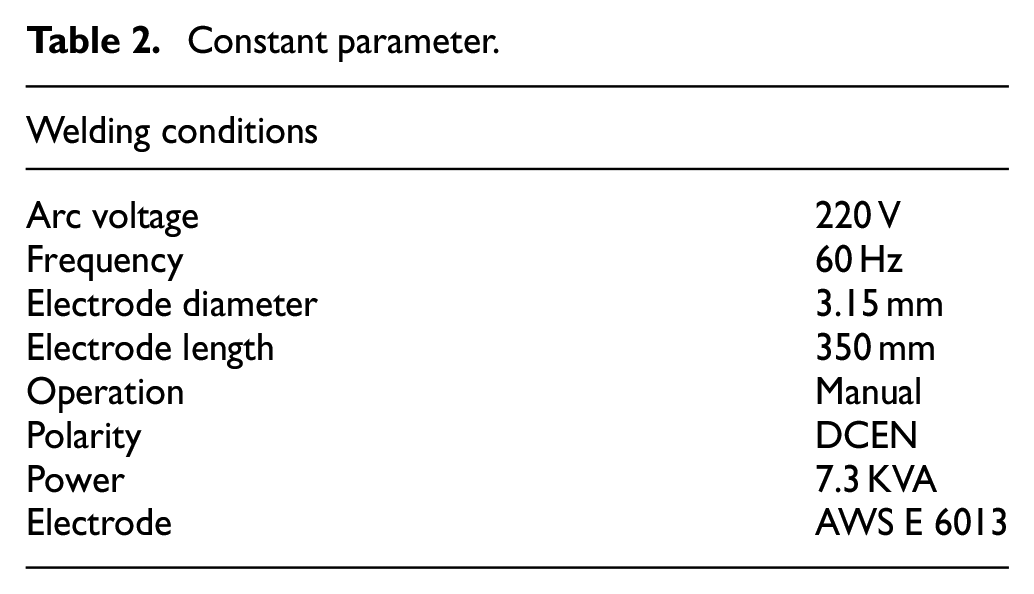
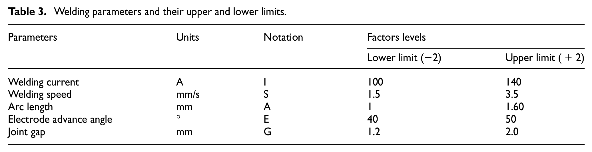
Experiments welding conditions are depicted in Table 2. These are constant parameters. The working range that is, minimum and maximum level of parameters is depicted in Table 3.
Constant parameter.
Welding parameters and their upper and lower limits.
The coded values for the intermediate range is calculated from the relation 21 shown in equation (1).

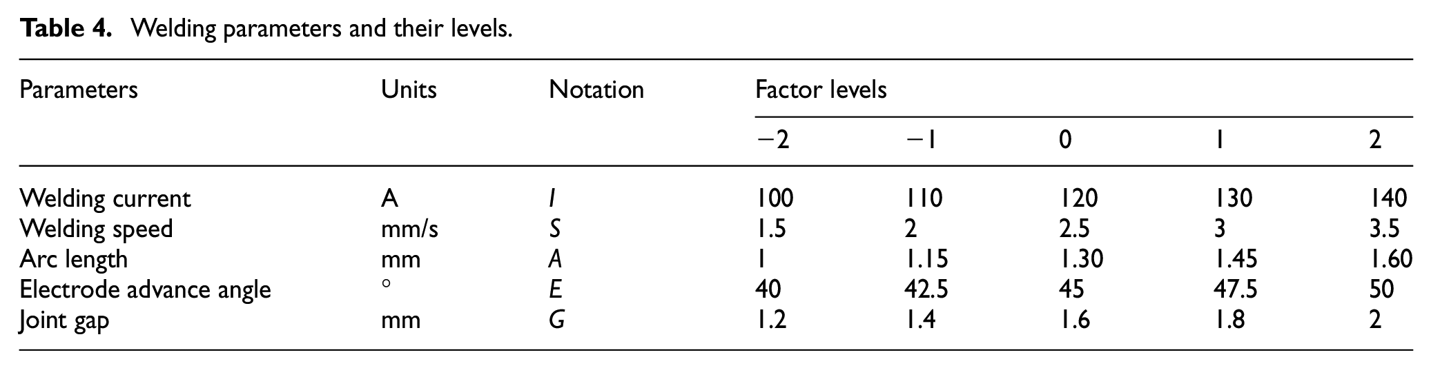
Where Xi is the required coded value of a ith variable X. X is any value of variable from Xmin to Xmax, Xmin and Xmax are lower and upper limits of the variable X, respectively. The decided levels of the selected process parameter with their units and notations are provided in Table 4.
Welding parameters and their levels.
The 32 specimen was welded as per design matrix which is shown in Figure 2.
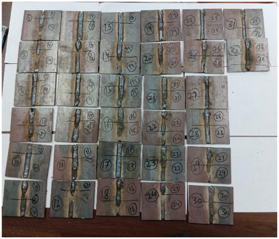
Thirty-two nos of specimen welded.
Measuring instruments
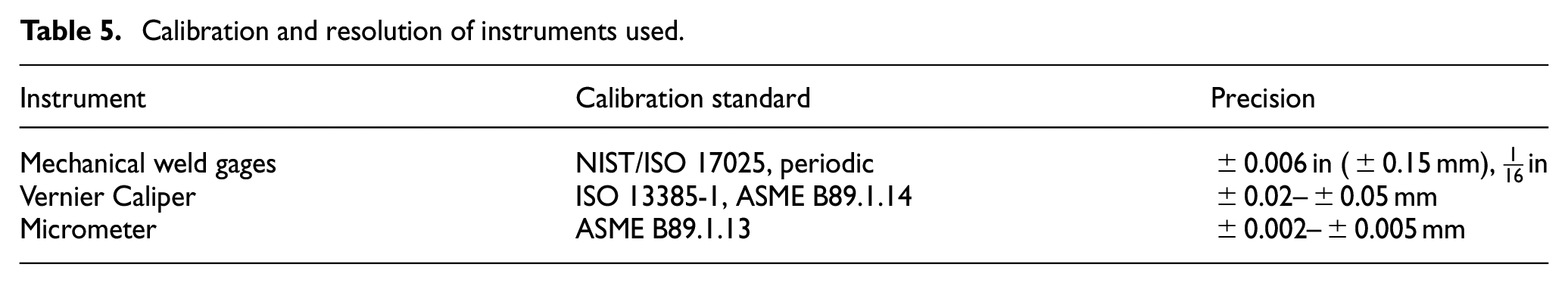
There are various measuring instruments which may be used for measuring the weld bead geometry characteristics. The laser, vision based instruments may be used which has higher resolution and calibration standards. In this study the mechanical weld gages, Vernier Caliper, micrometers are employed which characterized by right calibration and precision depicted in Table 5.
Calibration and resolution of instruments used.
Recording the responses
The experimental design matrix and measured responses has been shown in Table 6.
Design matrix and measured responses.

Development of mathematical model
The response function bead width (BW), reinforcement (R), penetration (P), weld penetration shape factor (WPSF), and weld reinforcement form factor (WRFF). Representing Y as the response, the response function can be expressed as shown in equation (2).
Y = f(Bead width, reinforcement, penetration, weld penetration shape factor, weld reinforcement form factor)

The second order polynomial (regression) equation used to represent the response surface Y for five factors is mentioned in equation (3).

and for five factors the selected polynomial could be expressed as shown is represented by equation (4).

Where, βo is the free term of regression equation, the coefficient β1, β2, β3, β4, β5 are linear terms, the coefficients β11, β22, β33, β44, β55 are quadratic terms, and the coefficients β12, β13, β14, β15 etc are the interaction terms. All the coefficients were calculated for their significance at 95% confidence level by using Minitab 22 statistical software package.
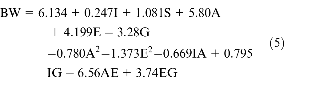
After determination of significant coefficients, mathematical models were developed by using these coefficients only after elimination of the insignificant coefficients. The final developed models for bead width, reinforcement, penetration, weld penetration shape factor, weld reinforcement form factor as mentioned in equations (5) to (9).
(i) Bead width
(ii) Reinforcement

(iii) Penetration

(iv) Weld penetration shape factor

(v) Weld reinforcement form factor

Checking the adequacy of developed model
The adequacy of developed models was checked using analysis of variance technique. This includes
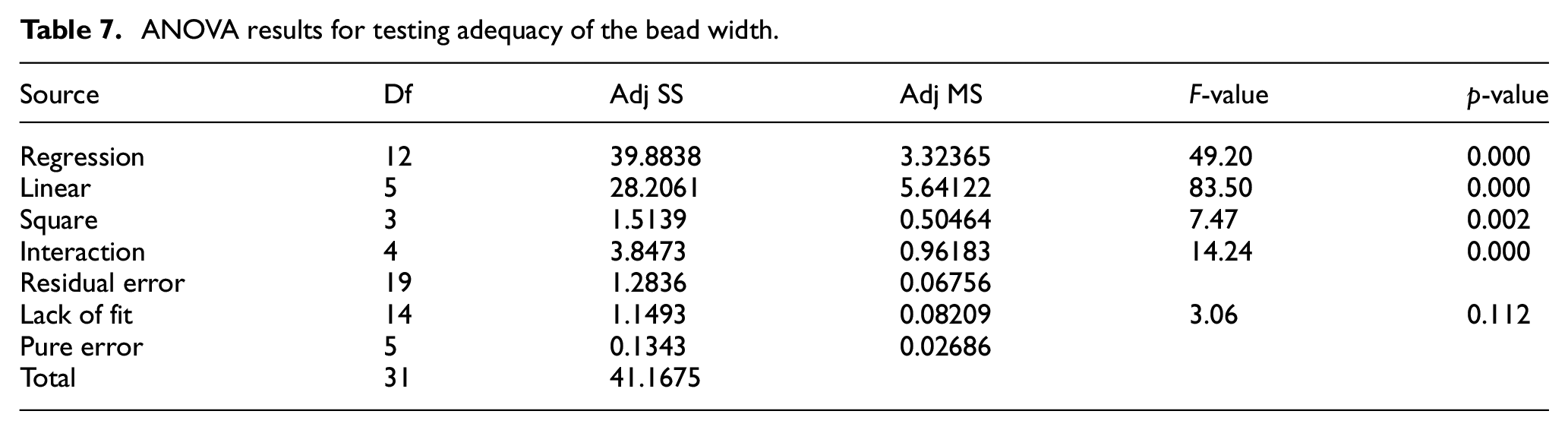
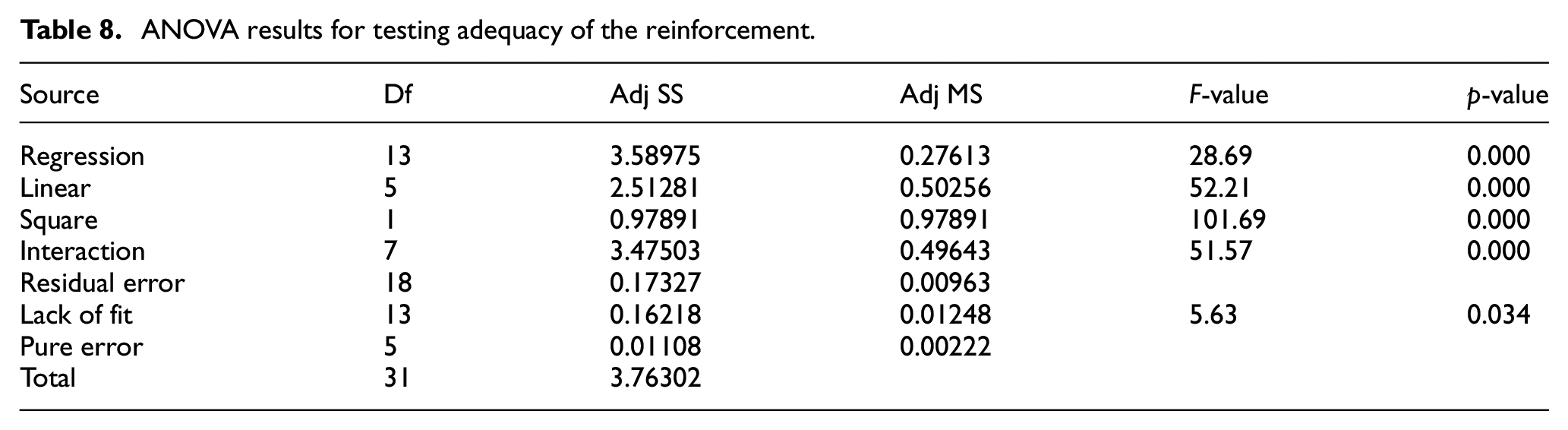
(i) The results of ANOVA (Tables 7–11) show the regression is significant with linear, square and interaction terms for five models (p-value is less than 0.05)
(ii) The models are found to be adequate as F-value is significantly larger than F-table value of each model which shows models are highly significant
(iii) Another evidence of the adequacy of models is significant lack of fit (p-value less than 0.05) which shows almost negligible lack of fitness of model.
ANOVA results for testing adequacy of the bead width.
ANOVA results for testing adequacy of the reinforcement.
ANOVA results for testing adequacy of the penetration.

ANOVA results for testing adequacy of the weld penetration shape factor.

ANOVA results for testing adequacy of the weld reinforcement form factor.

The evidence which indicates the correlation between the full and reduced models is that the values of R-sq and R2adj has no major difference. The values are depicted in Table 12.
Values of R-sq and R2adj.

Weld parameter optimization using Jaya (JA) algorithm
The Jaya is the novel swarm based heuristic algorithm developed by Rao. 22 It is the combination of evolutionary algorithms based on Darwin theory natural selection of the survival of the fittest as well swarm intelligence in which the swarm follows the leader during search of optimum solution. There are two principle approaches which has been used to find the solution. But in both the evolutionary and swarm based intelligence, the most appropriate thing is one has to be the fittest who finds the solution, but it may be defeated by the team approach which may bring the food closer. That where some algorithms have been worked on. That’s why Jaya is updated and it is not solely following the evolutionary approach (EA) but swarm approach also. In EA approach one person has its say entirely. It may be defeated, but as team approach, bigger solution can be worked upon. In this a candidate solution moves closer to the best solution in every generation, but at the same time a candidate solution moves away from the worst solution. In this candidates step by step gets closer to solution and keeping away or demarcating the worst solution in each iteration. Thereby, a good exploration and exploitation of the search space is achieved.
For the objective function of bead width, reinforcement, penetration, weld penetration shape factor and weld reinforcement form factor for each candidate. The calculation for Ist iteration as follows

Where X is candidates 1–5,
r 1 and r2 are two random numbers,
we will operate the fitness value for candidate one. Then perform greedy selection
If
In maximization if
Proposed steps used in JA as:
Initialize the parameters like population size and maximum iterations
Find the Xbest and Xworst as best and worst objective response
Compute the Xnew as per equation (10)
Check bounds
Perform greedy selection that is, f(Xnew) is better or not. If yes, update the solution
Set iteration = iteration + 1 and go to step above.
The proposed steps are depicted in Figure 3.

Flow structure of JAYA algorithm based on DOE.
The parameter of JAYA algorithm for computation are described in Table 13.
The parameter of JAYA algorithm for computation.

Numerical illustration of developed Jaya model
From the process of initialization to the calculating and finding out the refined and tuned values of five objective functions, the numerical illustration of developed Jaya is described here.
Initialization
From the Table 3, the upper and lower limits are used to initialize the solution using equation (11).
Initialize solution

Random numbers = [0.20, 0.25, 0.30, 0.35, 0.40]
Evaluation
The COF (Combined objective function is represented by equation (12).
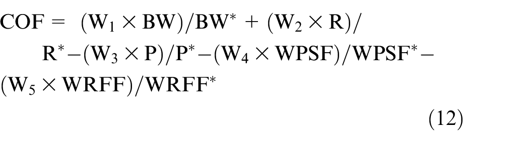
Where BW*, R* are minimal values of objective function of five candidates obtained by putting the values in mathematical model of bead width and reinforcement. P*, WPSF*, WRFF* are the maximum values of objective function of five candidates obtained by putting the values in mathematical model of penetration, weld penetration shape factor and weld reinforcement form factor which is depicted in Table 14.
Initial population
Calculated values and fitness for initial population with weights, W1 = 0.2, W2 = 0.2, W3 = 0.2, W4 = 0.2, W5 = 0.2.

Where f(x) = fitness function.
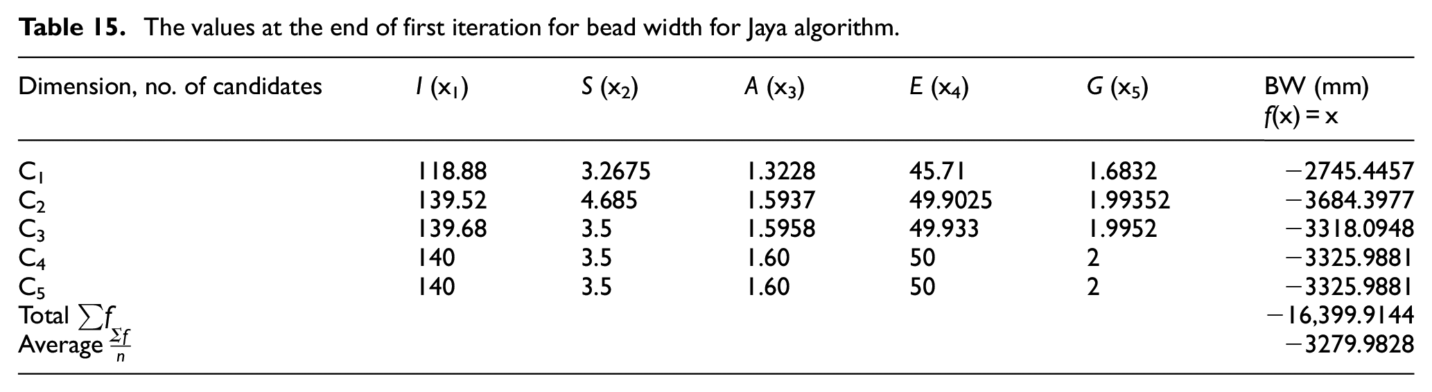
The solution obtained for bead width at the end of first iteration is depicted in Table 15 which is being obtained using equation (10).
The values at the end of first iteration for bead width for Jaya algorithm.
Similarly, the values obtained for reinforcement, penetration, weld penetration shape factor, weld reinforcement form factor at the end of first iteration is depicted in Tables 16 to 19.
The values at the end of first iteration for reinforcement for Jaya algorithm.

The values at the end of first iteration for penetration for Jaya algorithm.

The values at the end of first iteration for weld penetration shape factor.

The values at the end of first iteration for weld reinforcement form factor.

The solution obtained at the end of second iteration for bead width is shown in Table 20.
The values obtained at the end of second iteration for bead width.

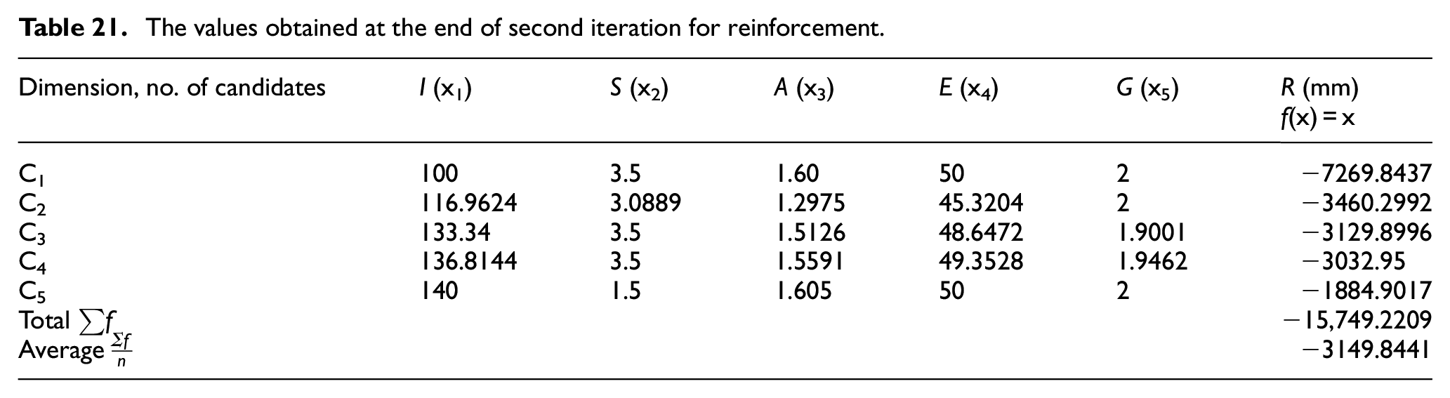
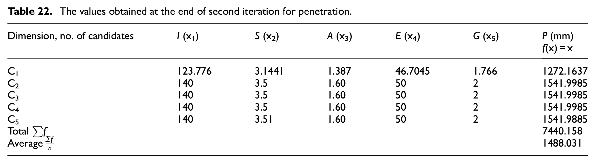
Similarly, the values obtained for reinforcement, penetration, weld penetration shape factor, weld reinforcement form factor at the end of second iteration is depicted in Tables 21 to 24.
The values obtained at the end of second iteration for reinforcement.
The values obtained at the end of second iteration for penetration.
The values obtained at the end of second iteration for weld penetration shape factor.

The values obtained at the end of second iteration for weld reinforcement form factor.

Weld parameter optimization using Firefly (FA) algorithm
The firefly algorithm (FA) developed in 2008 by Xin-She Yang 23 from Cambridge university. The algorithm developed based on the flashing behavior of fireflies and inspired to develop the metaheuristic algorithm. It is based on the principle of the evolutionary nature (EA) which is the unisex behavior of two fireflies, the one who is less brighter gets attracted by the more brighter fly. In second rule principle to find the solution, the population based fitness function will be partnered with the best bright firefly as the rule suggest attractiveness is proportional to brightness, as the brightness decreases due to increase in distance, their attractiveness also decreases. In next principle, to get the optimum value of objective function is directly related to the intensity of brightness. Based on these principles, the FA algorithm works.
For the objective function of bead width, reinforcement, penetration, weld penetration shape factor and weld reinforcement form factor for each firefly. The calculation for Ist iteration as follows

or

Where ,
Between 0 and 1
We will find the Xnew for each firefly for objective function by find the Xj which is minimum in case of minimization and maximum in case of maximization.


where xn and ynn = 1–5, are the values corresponding to each firefly population represented by Xi for x-values and Xj for y-values.
Then perform greedy selection
If
In maximization if
Proposed steps used in FA algorithm as:
Initialize the population using dimension of 5, number of iteration of 20
Find Xi, Xj, and r
Put the values of constants
Check bounds
Perform greedy selection that is, f(Xnew) is better or not. If yes, update the solution
Set iteration = iteration + 1 and go to step above
The proposed steps are depicted in Figure 4.

Flow structure of firefly algorithm based on DOE.
The parameter for firefly algorithm computations are described in Table 25.
The parameter of firefly computations.

Numerical illustration of developed firefly model
Initialization
Initialization of solution is done using equation (11).
Random numbers used for initialization = [0.45, 0.55, 0.65, 0.75, 0.85]
Evaluation
The combined objective function using equation (12) is shown in Table 26.
Initial population
Calculated values and fitness for initial population with weights, W1 = 0.2, W2 = 0.2, W3 = 0.2, W4 = 0.4, W5 = 0.2.
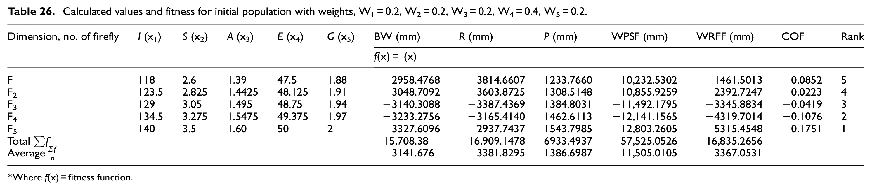
Where f(x) = fitness function.
The solution obtained for bead width at the end of first iteration is depicted in Table 27.
The values at the end of first iteration for bead width.

Similarly, the values obtained for reinforcement, penetration, weld penetration shape factor, weld reinforcement form factor at the end of first iteration is depicted in Tables 28–31.
The values at the end of first iteration for Firefly algorithm.

The values at the end of first iteration for Firefly algorithm.
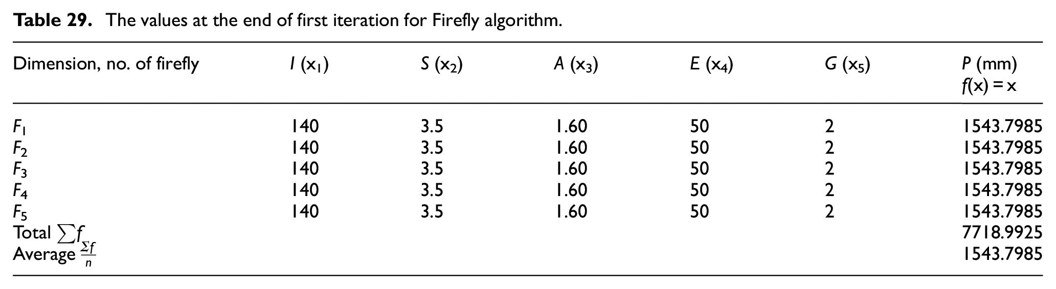
The values at the end of first iteration for weld penetration shape factor for Firefly algorithm.

The values at the end of first iteration for weld reinforcement form factor for Firefly algorithm.

Result and discussion
Figure 5 represents the combined objective function of each candidate which depicts rank of candidates obtained in Table 14.

The histogram chart showing the ranks of candidates according to the combined objective function.
In Figure 6 each objective response values is represented with two figures. The first figure represents the pictorial representation of fitness function values which shows the better values for JA and second figure describes the pie-chart which shows the change to better fitness function values after each iteration
(a-1) Bead width fitness values becomes better as the iteration increase, (a-2) Bead width pi(e)chart depicting better of fitness function values after each iteration, (b-1) Reinforcement fitness values becomes better with increase in iteration, (b-2) Reinforcement pi(e)chart depicting better of fitness function values after each iteration, (c-1) Penetration fitness values becomes better with increase in iteration, (c-2) Penetration pie-chart depicting better of fitness function values after each iteration, (d-1) Weld penetration shape factor fitness values becomes better with increase in iteration, (d-2) Weld penetration shape factor pie-chart depicting better of fitness function values after each iteration, (e-1) Weld reinforcement form factor fitness values becomes better with increase in iteration, (e-2) Weld reinforcement form factor pi-chart depicting better of fitness function values after each iteration.
Figure 7 represents the combined objective function of each firefly which depicts rank of firefly obtained in Table 26.

The histogram chart showing the ranks of firefly according to the combined objective function.
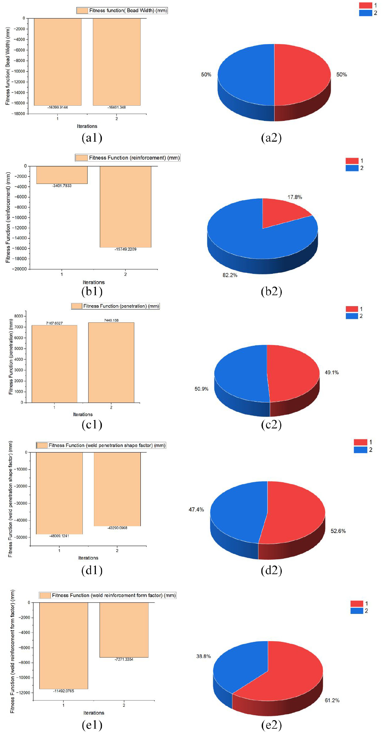
In Figure 8 each objective response values is represented with two figures. The first figure represents the pictorial representation of fitness function values which shows the better values for FA and second figure describes the pie-chart which shows the change to better fitness function values after each iteration

(a-1) Bead width fitness values becomes better as the iteration increase, (a-2) bead width pi(e)chart depicting better of fitness function values after each iteration, (b-1) reinforcement fitness values becomes better with increase in iteration, (b-2) reinforcement pi(e)chart depicting better of fitness function values after each iteration, (c-1) Penetration fitness values becomes better with increase in iteration, (c-2) Penetration pie-chart depicting better of fitness function values after each iteration, (d-1) Weld penetration shape factor fitness values becomes better with increase in iteration, (d-2) Weld penetration shape factor pie-chart depicting better of fitness function values after each iteration, (e-1) Weld reinforcement form factor fitness values becomes better with increase in iteration, (e-2) Weld reinforcement form factor pi-chart depicting better of fitness function values after each iteration.
The evolutionary and swarm based intelligence metaheuristic techniques are employed to optimize the parameters of shielded metal arc welding process. The objective is to find the better solution in each iteration. The JA algorithm worked to find the solution through the fittest person which could find the solution, but it takes into consideration the swarm which could find the solution. It worked to how often they find the solution and how they find the solution. After updating, there position they come closer to the optimal solution. In FA algorithm, it works on the brightness of the firefly, higher the brightness more the attractiveness which other fireflies with less brightness partenered with the brighter fly, so due to this an optimal solution is reached. In JA algorithm technique illustrated using Figure 6(a-1) depicts the fitness function values obtained from iteration from 1st to 2nd. The pie-chart also shows the values. In Figure 6(b-1) depicts better fitness function values from iteration 1st to 2nd . The pie-chart represents the values at iteration Ist is 82.2% and iteration 2nd is 17.8%. The values are better by 64.4%. In Figure 6(c-1) depicts the better values of fitness function for penetration. The figure depicts the better values obtained of fitness function from iteration 1st to 2nd. The pie-chart depicts the better values of fitness function at iteration 1st is 50.9% to 2nd 49.1%. The better change difference is of 1%. Similarly for weld penetration shape factor and weld reinforcement form factor, the better change difference is 5.2% and 22.4%. Therefore, it is clear that overall objective function is changing, which leads to optimal solution in JA.
In FA, technique illustrated in Figure 8(a-1) depicts the histogram which shows the fitness function values becomes better from initial population to iteration 1st. The pie chart depicting in Figure 8(a-2) shows better by value of 10%. Similarly, for reinforcement, penetration, weld penetration shape factor and weld reinforcement form factor the fitness function values becomes better by 4.4%, 5.4%, 1%, and 10.6%.
Effect of parameters on weld bead geometry
The Figure 9 depicts, effect of parameters on bead width. It shows as the current increases the bead width increases. This is due to higher heat input. With increase of welding speed and joint gap, the bead width decreases but with increase of arc length and electrode advance angle, the bead width increases, this is due to the fact that, higher arc length and higher electrode advance angle the heat input cover increases which increases the fusion zone and bead width increases.
The Figure 10 depicts the effect of parameters on reinforcement. It shows that as welding current, welding speed, electrode advance angle increases, the reinforcement decreases. This is due to the fact that higher current, the heat input increases but with high welding speed the heat input decreases and deposition rate also decreases. The higher electrode advance angle directed and started the arc which decreases the reinforcement. The reinforcement remains constant with increase in arc length and decreases with increase in joint gap. As arc length increases, higher deposition rate is achieved and with reinforcement decreases as distance between two plates increases.
Figure 11 depicts the effect of parameters on penetration. The figure depicts with increase in welding current, electrode advance angle and joint gap the penetration decreases and with increase of welding speed and arc length, the penetration increases. With increase of welding current, electrode advance angle and joint gap, the larger area needs to be accessed therefore, the penetration decreases. As welding speed and arc length increases, which narrow down the region and therefore penetration increases.
The Figure 12 depicts, the effect on parameters on weld penetration shape factor. The figure demonstrates that with increase in welding current and electrode advance angle, the weld penetration shape factor increases, this is due to the fact that higher heat input and well directed arc leads to increase in weld penetration shape factor. Further with increase in welding speed, arc length and joint gap, the weld penetration shape factor decreases, this is due to the fact that heat input per unit length decreases which decreases weld penetration shape factor.
The Figure 13 depicts the effects of parameters on weld reinforcement form factor. From the graph it is shown that as welding speed and joint gap increases, the weld reinforcement form factor decreases. This is due to the fact that higher welding speed decreases the heat input and higher joint gap increases the area of filling, this decreases the weld reinforcement form factor. Further higher welding current, arc length and electrode advance angle increases the weld reinforcement form factor. This is due to the fact that well directed with higher melting of coated electrode is obtained which increases the weld reinforcement form factor.

Effect of parameters on bead width.
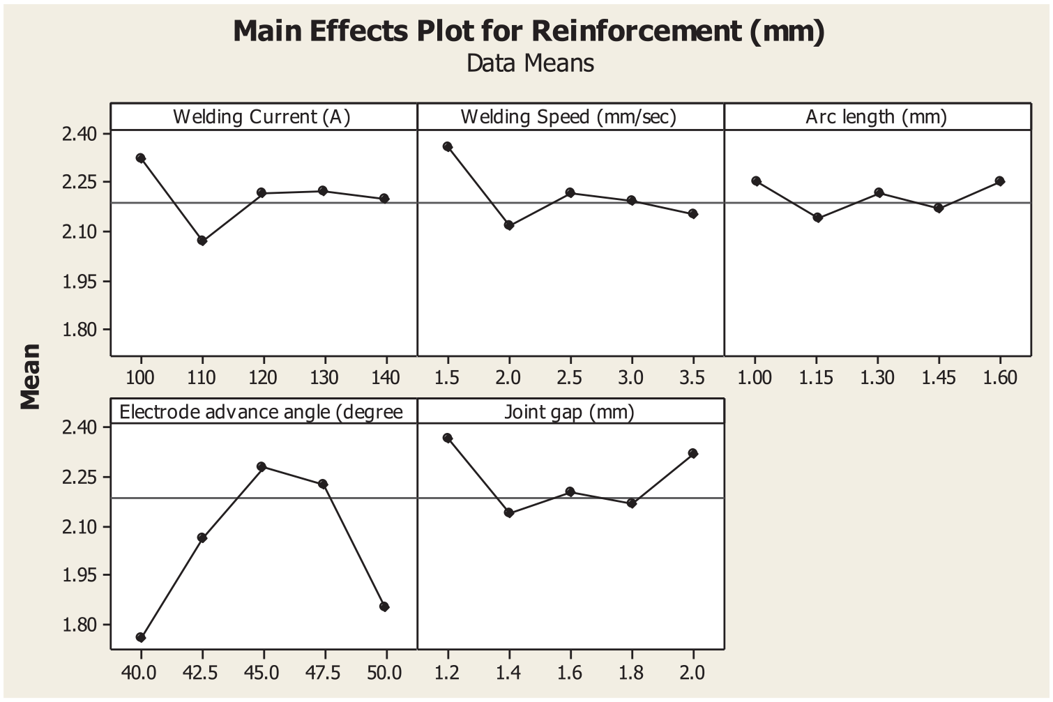
Effect of parameters on reinforcement.

Effects of parameters on penetration.
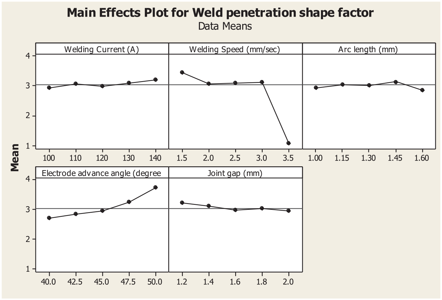
Effect of parameters on weld penetration shape factor.

Effect of parameters on weld reinforcement form factor.
Sensitivity analysis
The sensitivity analysis shows the effect of variations in input parameters influence the output results. The sensitivity analysis is carried out in software GoldSim 15, the table data from 14 to 31 is used to find the effect of input variable on the output response. The result depicted in Figure 14 that the welding current and welding speed are two parameters which effect the output response.
Tornado chart for sensitivity analysis. (a) BW. (b) R. (c) P. (d) WPSF. (e) WRFF.
The XY plots for output response is depicted in Figure 15. This plots depicts the variations in input variable effecting output response. The figure describes the change in welding current changes the output of the process.

Depicting XY plot which shows how changes in input variable (X-axis) effect the output response (Y-axis). (a) BW. (b) R. (c) P. (d) WPSF. (e) WRFF.
The Figure 16 depicts the distribution chart for each output response. It represents the variability in outcome. The figure depicts the larger spread with uniform distribution of data. This shows that each outcome reflects the effect on bead geometry characteristics.

Distribution chart depicting effect of input variable on output response (a) BW. (b) R. (c) P. (d) WPSF. (e) WRFF.
The sensitivity analysis result is depicted in Supplemental File.
Confirmation test
The results obtained from response surface methodology are compared with the results obtained from Jaya and Firefly algorithm. It was found that with these algorithms the values obtained for objective function is greater than the values obtained with response surface methodology. Further the optimal process parameters obtained is within the permissible limits. These values have been found comparable with the experimental results. The results has been depicted in Table 32.
Confirmation test results.

Wn: inertia weights.
The comparison with the previously studies done on bead geometry is depicted in Table 33.
Comparison of weld bead geometry with previous studies.

The Figure 17 describes the axial, homogeneous and refined grains obtained after nucleation

Microstructure of weld bead at (a) 200 µm and (b) 50 µm.
From the results it has been clearly indicated that with Jaya and firefly algorithm the results are much improved. The bead width, reinforcement decreases and penetration increases. The microstructural and mechanical properties depend upon the weld bead geometry characteristics. The weld width increased with greater current and energy densities and reduced the tensile properties. High welding travel speed produces more elongated weld pool and continuous contour resulted in “V” shape. A significant amount of homogeneous, refined and axial nucleation was observed in FZ center of these welds because of low current. In addition to this low welding travel speed produced C-shaped ripples and few axial grain nucleation sites in the FZ. The latter was evidence of a slower solidification rate. The dendrite like secondary arm spacing measurements confirmed this hypothesis. It was observed that axial grains in the FZ center improve the weld bead tensile properties. 27
Real-world verification
The real world verification tells that the values of input variable are obtained after optimization. The GoldSim 15 software is applied in which the regression model of output response is used as data. The values obtain of input at the trails mentioned for each output variable depicted in Figure 18 is obtained after iterations and is found to be similar (depicted in trails) with that of values obtained in JA and FA obtained in Table 32. They are very close and within the maximum and minimum permissible limits.

Optimized values of input variables for the output response after certain iterations. (i) BW (trail 1 and 3). (ii) R (trail 1 and 5). (iii) P (trail 48 and 42). (iv) WPSF (trial 45 and 43). (v) WRFF (trial 50).
The optimized results have various advantages like there is no need of extensive trail -and-error on the shop floor. The welding cycles are faster, less material waste and higher overall efficiency. The models developed from AI and machine learning in laboratory setting can predict the optimal parameters for different material and joint types ensuring consistent weld quality and minimizing defects like porosity or cracking. Through the computations and data processing they are predicting the optimized values. The optimized results can be implemented in robotic welding system.
But in SMAW the use of robotic welding system does not arise as it cannot be performed by robots due to its equipment features. These are the average of two readings obtained so there are two replicates which were obtained. The results are the average of two replicate readings. Therefore, the error in results are minimized. In industrial settings in any SMAW welding machine the welding variables will be similar. Therefore, the results can be replicated in any SMAW machine in the industry. The industries are using the real time monitoring data which helps in understanding and predicting the future behavior of the system in the environment. In optimization it used to fine tune the parameters values to obtain the optimum results. It is very static.
Conclusion
Design of experiment was conducted to find out the optimized results. These regression model used are being used as objective function to find out the optimized results using JA and FA as described in Table 32. The results indicate that all five independent controllable process parameters optimized has values between minimum and maximum values of controllable process variables. Further better optimized results are obtained by JA and FA. This results shows that JA is the powerful tool in experimental SMAW optimization
The foremost importance of JA is that it utilizes both theory of survival of the fittest and swarm based intelligence to obtain the best solution. This ensures that the solution does not move to local optima, it reaches to global optima. Further it ensures that solution is reached at minimum iterations which is suitable to find solution in large search space like SMAW. Confirmatory test results proved that there was good agreement between the experimental and predicted results.
The main advantage of FA algorithms is that it utilizes the partner function to reach the solution at a faster rate. So it utilizes the qualitites of partner to reach the solution in the search space So it is used not only for SMAW but also for GTAW, robotic welding etc.
This work can be extended further to solve problems in other manufacturing process like machining, forming etc.
Supplemental Material
sj-docx-1-ade-10.1177_16878132251356567 – Supplemental material for Optimization of shielded metal arc welding process parameters on weld bead geometry using Jaya algorithm and Firefly algorithm
Supplemental material, sj-docx-1-ade-10.1177_16878132251356567 for Optimization of shielded metal arc welding process parameters on weld bead geometry using Jaya algorithm and Firefly algorithm by Pushp Kumar Baghel in Advances in Mechanical Engineering
Footnotes
Handling Editor: Sharmili Pandian
Author contributions
The manuscript is designed and written by Dr. Pushp Kumar Baghel. From the conceptual design to material preparation, data collection, analysis, framework etc were performed by Dr. Pushp Kumar Baghel. In case of any query contact Dr. Pushp Kumar Baghel at
Funding
The author received the research grant for paying Article Processing Charges for publication of this article from Guru Gobind Singh Indraprastha University, East Delhi Campus, Delhi-110092.
Declaration of conflicting interests
The author declared no potential conflicts of interest with respect to the research, authorship, and/or publication of this article.
Data availability statement
All data generated or analyzed during this study are included in this published article
Research involving human participants and/or animals
This article does not contain any studies with animals performed by any authors
Supplemental material
Supplemental material for this article is available online.
References
Supplementary Material
Please find the following supplemental material available below.
For Open Access articles published under a Creative Commons License, all supplemental material carries the same license as the article it is associated with.
For non-Open Access articles published, all supplemental material carries a non-exclusive license, and permission requests for re-use of supplemental material or any part of supplemental material shall be sent directly to the copyright owner as specified in the copyright notice associated with the article.