
Abstract
Due to the advancement of driverless technology, multi-vehicle cooperation and intelligent travel will become the key direction of intelligent transportation system technology. In high-level autonomous driving, the elimination of intersection signals can effectively improve the efficiency of road traffic. For unsignalized intersection scenarios, considering whether vehicles arrive simultaneously, we propose single-phase and multi-phase trajectory planning methods for multi-vehicle cooperative motion based on numerical optimization techniques. This method includes establishing a vehicle kinematic model, considering the constraints of the vehicle’s physical system and boundary conditions, and developing effective multi-vehicles collaborative motion obstacle avoidance strategies. The trajectory planning task is described in the form of an optimal control problem, and the optimal trajectory is obtained by numerical optimization with the shortest passing time to complete the intersection as the optimization objective. Through numerical simulation analysis of intersection scenarios including crossroad and roundabout, the results demonstrate that the proposed algorithm can achieve optimal trajectories for multi-vehicle cooperative motion while ensuring safe vehicle operation, which improves the efficiency of future intelligent traffic networks.
Keywords
Introduction
The Intelligent Transportation System (ITS) is based on sophisticated infrastructure, effectively integrating advanced information technology, communication technology, sensing technology, control technology, computer technology, and other innovations into the entire transportation management system. 1 It can greatly improve the travel experience of city dwellers. Vehicles in future ITS may have L5-level autonomous driving capabilities, 2 it can completely replace manual driving in any environment and achieve all-weather unmanned driving, so intersections geared toward ITS can be controlled without signals. In the whole road network, intersections are crucial hubs in the road network where vehicles converge, turn, and disperse. They play a critical role in overall traffic safety. 3 Figure 1 is a conceptual diagram of a future unsignalized intersection. When vehicles pass an intersection without signal lights, they can sense the surrounding driving environment through the roadside unit V2I and V2V technology. Through cloud-based supercomputing, vehicles execute cooperative motion decision-making tasks among multiple vehicles, ensuring efficient intersection passage without human intervention. 4 This technology development will help improve road traffic safety and enhance traffic efficiency.

Unsignalized intersection model.
The decision planning of multi-vehicle cluster cooperative movement is the key to realize the above-mentioned technology. The current mainstream methods of autonomous driving motion planning are divided into five categories, graph search method, geometric line method, random sampling method, reinforcement learning method, and numerical optimization method. The common algorithms are Dijkstra algorithm and A* algorithm. The improved A* 5 obtained a shorter path length, fewer inflection points and smoother, which can avoid the collision between the vehicle contour and the obstacle. The graph search method can quickly obtain the driving path, but the planning results are relatively rough. The graph search method is usually used as a preprocessing for other methods. In literature, 6 according to the geometric relationship between vehicles, surrounding obstacles, and target parking Spaces, geometric methods such as tangent arcs and straight lines were used to obtain parking paths. This method has the advantages of simple algorithm and high solving efficiency, but the curvature of the planned path is discontinuous. The random sampling method generates paths at random sampling points in the configuration space. Based on the RRT algorithm, literature 7 used the target offset strategy and the pruning optimization algorithm to greatly shorten the length of the path planning and the path search time. However, the random sampling algorithm has poor ability to accurately deal with complex constraints. Machine learning algorithms learn path planning models based on a large amount of training data. The advantage of machine learning algorithm is that it has fast calculation speed and certain generalization ability, but it needs to collect a large number of training samples. Literature 8 proposed a deep neural network (DNN)-based trajectory planning method for both parallel and perpendicular parking scenarios, and the presented strategy was able to theoretically guarantee the stability of the control scheme and the convergence of the tracking error. For the autonomous parking problem, an algorithm based on polynomial parameterization and genetic algorithm optimization was proposed in the literature. 9 In literature, 10 trajectory planning of intelligent vehicles (ICVs) in cooperative driving environment is discussed, and an adaptive trajectory planning method named AdaTP was proposed. Results demonstrated that this method can generate shorter and more reliable trajectories. Literature 11 introduced the localized trajectory planning problem for Automated Guided Vehicles (AGVs), and adopted reinforcement learning method based on double delay depth deterministic strategy gradient (TD3) to improve the performance and efficiency of trajectory planning. Literature12,13 proposed a new reinforcement learning strategy to realize vehicle trajectory planning, which verified the superiority of the algorithm. The results had great significance for the practical implementation in actual scenarios.
The essence of vehicle motion is to solve the problem of dynamic system, by describing the dynamic characteristics of the vehicle and constructing the equation of the dynamic system, together with the constraints and the objective function, the optimal control problem is constituted. The research shows that the optimal control problem can describe the vehicle trajectory planning problem intuitively and accurately, which is not possessed by other methods. 14 The overall idea of numerical optimization methods is to transform the vehicle motion planning problem into an optimal control problem, and then the optimal control problem is discretized into a nonlinear programming problem through the numerical optimization algorithm. Subsequently, the optimization problem is solved using gradient descent methods to obtain the planning results. This method is characterized by fast convergence speed and low sensitivity to initial value. This method is characterized by fast convergence speed and low sensitivity to initial value. The numerical optimization method can obtain the position, velocity, acceleration, heading angle, and other time-related parameters of the vehicle movement, which can be directly used for low-level tracking control of vehicles. Meanwhile, the objective function can be set to obtain the vehicle trajectory with the shortest time. Therefore, this paper adopts the numerical optimization method to solve the multi-vehicle cooperative trajectory planning problem. Literature 15 introduced an optimization method for planning fast maneuvers of trailer vehicles in twisting and narrow tunnels. An optimization-based maneuver planner is proposed, which had obvious advantages over the popular sampling and search-based planners. Literature 16 proposed a cooperative trajectory planning method for vehicle cut-through scenarios based on optimal control. This method used a fifth-degree polynomial to generate an initial solution to the optimal control problem. The purpose of this approach was to ensure that connected intelligent vehicles (CAVs) can merge into the main road quickly and efficiently. Literature 17 described a hierarchical control algorithm for self-driving vehicle trajectory planning and tracking based on Model Predictive Control (MPC) and Gaussian Pseudo-spectral Method (GPM). The article validated the effectiveness and feasibility of the algorithm through simulations and real vehicle tests. In literature, 18 the optimal trajectory planning for autonomous parking time of tractor semi-trailer based on segmental Gaussian pseudo-spectrum method is proposed. Compared with the traditional pseudo-spectrum method, this method can obtain shorter parking time and significantly increase the convergence speed.
Multi-vehicle cooperative motion planning refers to the process of solving paths or trajectories for multiple cars, given their initial motion states, destinations, and constraints. 19 In centralized control, the central computing control unit makes decisions by collecting all the controlled vehicle information and environmental information, and then distributes the optimal control sequence signal to the corresponding controlled vehicle and executes it. Centralized control can effectively formulate the optimal control problem for the entire system, and the global optimal solution can be obtained through the top-level control strategy. A multi-vehicle formation trajectory planning method is proposed in literature, 20 and the simulation results showed that vehicles can save a lot of passing time under high traffic volume. Literature 21 proposed a multi-vehicle cooperative autonomous parking trajectory planning based on connected fifth degree polynomials and genetic algorithm optimization, which can be significantly reduced overall stopping time. Literature 22 introduced a method for multilane unsignalized intersection cooperation. This method took flexible lane directions by calculating the two-dimensional distribution of vehicles and planning conflict-free vehicle crossing of the intersection. Literature 23 proposed a hierarchical multi-vehicle cooperative motion planning method based on interactive spatio-temporal corridors (ISTCs), and simulation experiments are conducted under unsignalized intersections to verify the feasibility of the framework. For the Autonomous Intersection Management (AIM) problem, Li et al.24–26 modeled the multi-vehicle coordination problem as a centralized optimization problem, and used batch processing or phased strategy to reduce the computational complexity. The availability of the obtained theoretical results was verified by simulation experiments, which improved the efficiency and fairness of vehicle traffic. Li and Zhang 27 proposed a fault-tolerant centralized collaborative optimization motion planning method for networked autonomous vehicles (CAVs). The path adjustment effect of the vehicle under different fault degrees is verified by numerical simulation, and the effectiveness of the method in some failure scenarios is demonstrated. The above research results have made a positive contribution to multi-vehicle collaborative trajectory planning. Literature 28 proposed a lane-free joint optimal control framework. Vehicles can freely use the two-dimensional space of the intersection to improve traffic efficiency and flexibility. At the same time, the acceleration, steering angle, fuel consumption, and expected speed tracking were simultaneously optimized in the objective function, which significantly improved passenger comfort. In this paper, a centralized frame algorithm is used to plan the path of multi-vehicle cluster motion. The innovations and research work of this paper mainly include: (1) A mathematical model of multi-vehicle cooperative motion is established, which includes the mathematical modeling of collision avoidance strategies between single vehicle and static obstacles, multi-vehicle and static obstacles, and between vehicles. (2) Taking the shortest vehicle passing time through the intersection as the optimization objective, the multi-vehicles centralized optimal trajectory planning for unsignalized intersections is transformed into a nonlinear optimal control problem, and then solved by numerical optimization method. Aiming at the complex mathematical model of the multi-vehicle cooperative motion trajectory solving problem, which cannot converge quickly. Based on the driving area of vehicles at the intersection, the process of multi-vehicle passing the intersection is divided into three phases, so as to narrow the scene range of trajectory solving at each phase, simplify constraints, and improve the convergence efficiency of the solution. At the same time, in the process of solving in phases, the continuity constraint problem of all vehicle control variables in different phases is solved, so as to ensure the one-time solution of multi-phase. Another advantage of solving in phases is that if there is a vehicle in the intersection that has not yet completely left the intersection in the next solution, it is sufficient to determine its phase in the next solution while preserving the continuity of the variables.
Vehicle motion process analysis
Individual vehicle kinematics modeling
In the early stages of intelligent transportation system, the vehicle is traveling in the working condition of urban intersection, considering the multi-vehicle safety problem, the vehicle traveling speed is low, it can be considered that all wheels are rolling state, and the effects of lateral forces on vehicles can be disregarded. Wheel slippage is not observed. Based on the Ackermann front-wheel steering principle, the vehicle kinematic model is established in a ground-fixed coordinate system, with the rear axle center point as the observed state variable.
In Figure 2,

Vehicle kinematics model.
According to the kinematic model, the differential equations describing the vehicle’s motion are as follows:

Where,
Constraint condition
Physical condition constraint
During vehicle driving, it is necessary to satisfy its own physical and mechanical constraints, which impose limitations on certain state variables, and control variables of the system as follows:
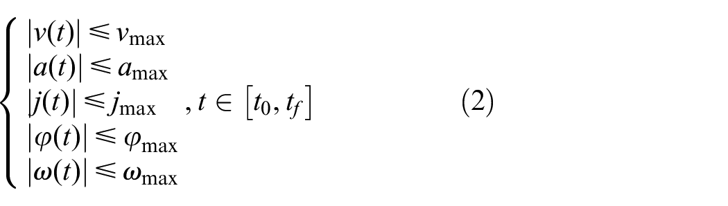
Where
Lane boundary constraints
In this paper, the intersection and roundabout conditions are selected, when vehicles pass through an intersection, one of the first external constraints they should consider are the boundary condition constraints. Vehicles move in the boundary area of the road, as shown in Figure 3,


Road boundary constraint diagram: (a) intersection and (b) roundabout intersection.
Vehicle obstacle avoidance constraints
When vehicles pass through intersections, they must avoid collisions with each other and must not collide with the road boundaries during their travel. Strict constraints are necessary for the vehicles’ trajectory. Due to the vehicle’s actual profile closely resembling a rectangle, a common constraint method is to use a quadrilateral to represent the vehicle’s trajectory. Based on the vehicle’s dimensions, rear axle center point position, and geometric relationships, the horizontal and vertical coordinate values of the four contour vertices of the vehicle can be derived. Here, an expanded rectangle is used to describe the contour of the vehicle, as shown in Figure 4.


Schematic diagram of vehicle movement obstacle avoidance at intersection.
When a rectangle is used to describe the vehicle profile, if it is necessary to meet that there is no collision between a vehicle and another vehicle, and the geometric meaning of this constraint on a two-dimensional plane is: at any moment, no point on the other vehicle falls within the rectangle outline of the own vehicle. As shown in Figure 4, the orange regions around the vehicle represent the safety threshold ensuring collision-free operation. If the vehicle does not collide with

Where

When the line

Where
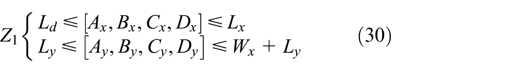
For road boundary obstacle avoidance, the first step is to describe the boundary contours of the intersection as four rectangles. And the orange region around the road contour is the safety threshold to ensure that the boundary does not collide with the vehicle, which are rectangles

When the line

When vehicles pass through roundabout intersections, it is necessary to consider collisions with the roundabout boundary. The center of the roundabout is point

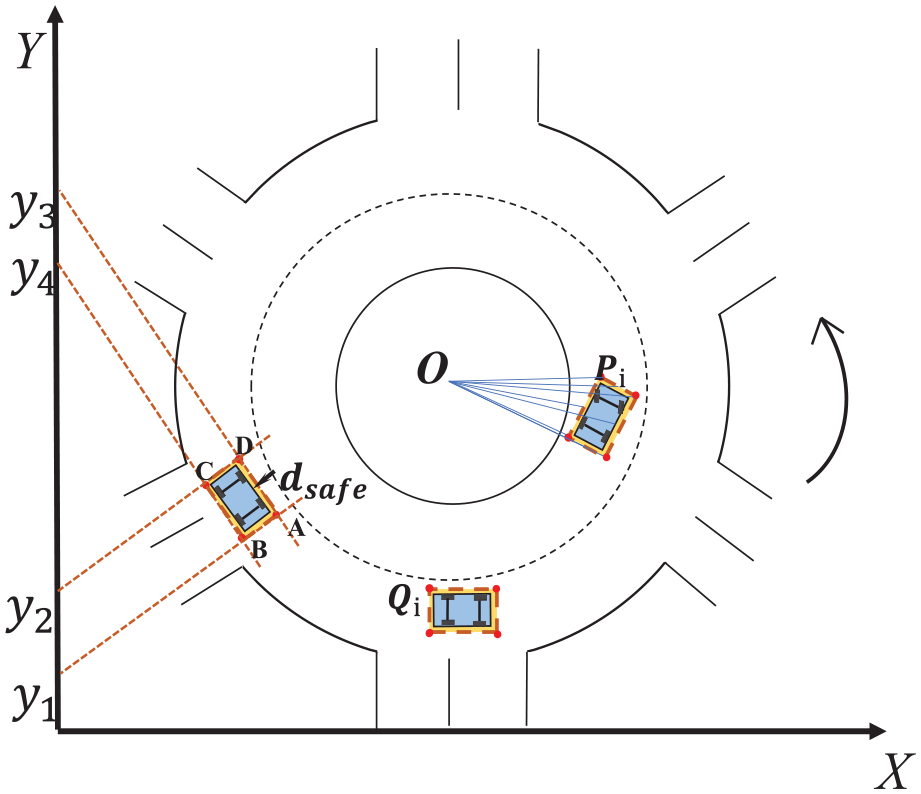
Schematic diagram for avoiding obstacles for vehicles traveling around the roundabout.
The vehicle collision constraint condition is the same as the obstacle avoidance of the vehicle at the intersection. Refer to equation (6). According to our traffic regulations, vehicles on traffic circle roads travel in a counterclockwise direction.
Multi-vehicle cluster cooperative motion trajectory planning
Description of multi-vehicle cluster cooperative motion problem
The optimal control problem typically contains the dynamics differential equations of the controlled system, path constraints, boundary constraints, and performance index function. The path constraints contain both equal and unequal constraints. Under the constraints satisfied by the controlled system, the optimal control parameters are obtained by solving the performance index function. The nonlinear optimal control Bolza problem can be described as:


In equation (11): the first row describes the differential equations of state of the system; the second row the unequal path constraints; the third row the equal path constraints; and the fourth row the boundary constraints, where


Multi-vehicle cooperative motion trajectory solution based on numerical optimization method
The numerical optimization is a method for solving nonlinear optimal control problems. This method discretizes the continuous optimization problem at Legendre-Gauss (LG) points, Lagrange interpolation polynomials are constructed to approximate state variables and control variables, and replaces differential equation constraints with algebraic constraints. Then the optimal control problem is transformed into Nonlinear Programming (NLP) problem solving. Numerical optimization methods are characterized by their high adaptability to initial values, fast convergence speed, and high solution accuracy.
Numerical optimization method can solve single-phase and multi-phase multi-vehicles trajectory planning problems. Single-phase trajectory planning refers to the vehicle trajectory planning for a direct solution, the vehicle departs from the starting point at the same time, and then arrives at the endpoint at the same time. However, vehicles can not only start at the intersection at the same time, but also start from the intersection in the process of other vehicles passing the intersection, at this time, the trajectory solving computation increases. In this case, single-phase trajectory solution cannot be realized. Therefore, multiple-phase are used to solve the problem, and each phase has its specific constraints. At the same time, it is necessary to add corresponding endpoint constraints at the boundary between multiple phases to maintain the continuity of the values of vehicle state variables and control variables. During segmented solving, collision avoidance constraints and endpoint constraints are simplified, which improves the success rate and convergence efficiency of multi-vehicle cooperative trajectory solving. For complex scenarios like intersections, where the arrival times of vehicles at the intersection are random, multi-stage trajectory planning can be employed to solve the problem.
Time domain transformation
The vehicle start-stop motion time range [
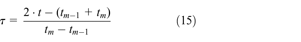
Through the time-domain transformation, the optimal control problem in the subinterval

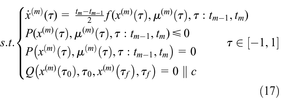
In equation (16),
Variable discretization
The above state and control variables are discretized at the Legendre-Gauss (LG) collocation points, and Lagrange polynomials at the discretization points are constructed to approximate the state variable

Taking the zeros
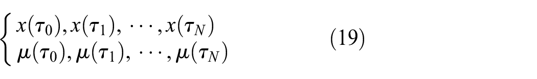
The Lagrange interpolation polynomial is constructed at

From equations (18) to (20), the approximate polynomial of the state variable and control variable in the subinterval

The derivation of equation (20) can be used to approximate the differential of the state variable by using the differential of the approximate polynomial. For example, the derivative of the state variable at the time point
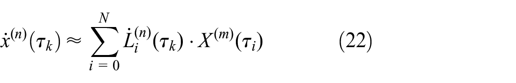
Combining equations (16), (17), and (22), the kinematic differential equation constraints can be converted into algebraic equation constraints:

Constraints under discrete conditions
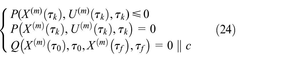
The equality and inequality constraints of the discrete system variables are as follows:
In the actual motion of vehicles, it is necessary to ensure the continuity of path curvature, thus the state variables must also be continuous change, that is, the requirement of the terminal moment of each sub-interval state variables and the next sub-interval of the initial moment of the state variables of the same value, but the change of the control variables can be discontinuous, the specific constraints are as follows:

As can be seen from equation (19), LG match points do not contain the terminal time of each subinterval, so the terminal state can be approximated by Gauss integral according to equation (25), and the approximate value of state variable at terminal time can be obtained as follows:

Where

Performance indexes under discrete conditions
Through the above discretization process, the optimal control problem for vehicle trajectory planning can be transformed into a nonlinear programming problem. The performance indexes under discrete condition is as follows:

In summary, through discretization at designated points, the Bolza optimal control problem is converted into a standard NLP problem, which provides a foundation for the approximate solution of the subsequent optimal control problems.
Phased solving of unsignalized intersections vehicle trajectory
Based on the driving area of vehicles at the intersection, the process of multi-vehicles passing the intersection is divided into three phases, so as to narrow the scene range of trajectory solving at each phase, simplify constraints, and improve the convergence efficiency of solution. At the same time, in the process of solving in phases, the continuity constraint problem of all vehicle control variables in different phases is solved, so as to ensure the one-time solution of multi-phase. As shown in the figure below, the dashed box indicates what we consider as the intersection range, and the vehicle enters the region to start the centralized trajectory solving. The first phase is that the vehicles move from the initial position to the area near the intersection, and at the same time, it will adjust the vehicle position and heading angle to facilitate further entry into the intersection area, which we call the entry into the intersection phase, and the corresponding traveling area is

Schematic diagram of the division of the intersection area.

Schematic diagram of the area division at the roundabout intersection.
The state variables of the vehicle at each phase junction should be constrained to ensure continuity.

Where

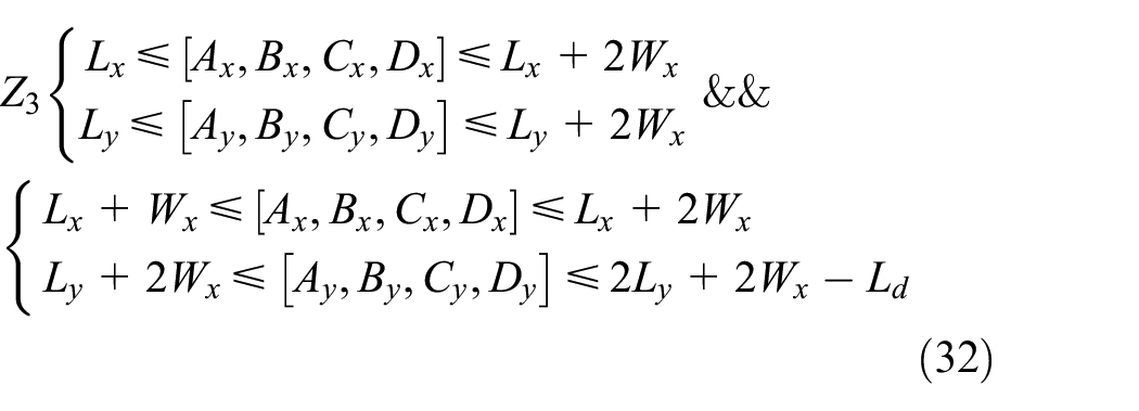
The following equations represent the constraint conditions for a vehicle to travel counterclockwise from the starting intersection and leave from the third roundabout intersection.


The algorithm for solving the unsignalized vehicle trajectory planning in segments is shown in Table 1 below.
Description of the segmentation algorithm.

Simulation and verification
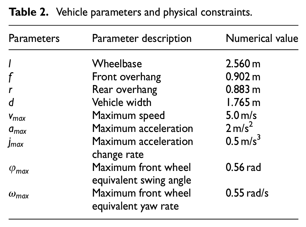
In the trajectory planning process, based on the vehicle’s kinematic model and constraints, the trajectory solution program based on numerical optimization method was written on the Matlab platform. The vehicle parameters and physical constraints are shown in Table 2.
Vehicle parameters and physical constraints.
Intersection and traffic circle intersection conditions are taken as examples. The trajectory planning algorithm based on numerical optimization method is verified and simulated. The simulation types are divided into single-phase multi-vehicle cluster and two-phase multi-vehicle cluster planning simulation.
The road at the intersection is set with lengths of 125 m in both directions, and the simulated roadway has six lanes in both directions with a lane width of 3

(a) Simulation results of single-phase trajectory planning at intersection, (b) simulation results of multi-phase trajectory planning at intersection, (c) simulation results of single-phase trajectory planning at roundabout, and (d) simulation results of multi-phase trajectory planning at roundabout.
The intersection single-phase vehicle simulation is set up with four groups, and it takes a total of 140.13
We set up a total of five batches for the multi-phase vehicle simulation at the roundabout intersection, each batch of vehicles passing through the intersection is divided into three phases, and all batches of all vehicles passed through the intersection in a total time of 106.9
https://www.bilibili.com/video/BV1de8gesEBX/.
The status parameters and control parameters of the vehicle are shown in Figure 9.

State parameter information of vehicles: (a) intersection single-phase trajectory planning, (b) intersection multi-phase trajectory planning, (c) single-phase trajectory planning for roundabout, and (d) multi-phase trajectory planning for roundabout.
The above results are the parameter information of one of the vehicles in each driving condition. From Figure 9, it can be seen that the planning results of the vehicle’s state and control parameters are strictly controlled within the constraints of Table 2. The vehicle starts from the starting point at an initial speed, accelerates to approximately its maximum speed, passes through the intersection at a relatively fast pace, then begins to decelerate after crossing the intersection to reach its final speed, and the speed and acceleration of the vehicle during the whole process are relatively stable.
Through the box plots, the relevant information about each vehicle can be displayed intuitively. The box plots of vehicle speed are shown below.
It can be seen from Figure 10(a) that the median speed of vehicles in a single phase at the intersection is above 4


Box plots of vehicle speeds: (a) single-phase trajectory planning at intersection, (b) multi-phase trajectory planning at intersection, (c) single-phase trajectory planning at roundabout, and (d) multi-phase trajectory planning at roundabout.
Figure 11(a) for the vehicle contour of the single circle description, equation (28) in

Description of the minimum safe distance between vehicles: (a) Normal posture between vehicles and (b)Vehicles are in a parallel posture in the Y direction.

Box plots of minimum inter-vehicle distances: (a) single-phase trajectory planning at intersection, (b) multi-phase trajectory planning at intersection, (c) single-phase trajectory planning at roundabout, and (d) multi-phase trajectory planning at roundabout.
It can be observed that for both intersection and roundabout scenarios, most of the minimum distances between vehicles at intersections and roundabout conditions are greater than 4.7
Conclusion
This paper proposes a numerical optimization-based method for multi-vehicle cooperative trajectory planning at unsignalized intersections. By establishing the vehicle kinematic model, physical system constraints, boundary condition constraints, and obstacle avoidance constraints, the vehicle trajectory planning problem is converted into an optimal control problem, taking the shortest vehicle crossing time as the optimal objective function, numerical optimization is applied to solve the multi-vehicle trajectory planning optimal control problem. This method realizes the obstacle avoidance strategy of multi-vehicle cooperative motion, according to the random departure of vehicles at the intersection, the above multi-vehicle trajectory collaborative planning problem can be solved in single-phase or divided into multiple-phase.
This paper performs trajectory planning for two scenarios: intersections and roundabouts, and carries out single-phase and multi-phase multi-vehicle trajectory coordination planning for each scenario. The simulation results show that the algorithm can converge to obtain the vehicle trajectories under the both working conditions, and the obtained trajectories are relatively smooth. Based on the statistical data from box plots of vehicle speeds and minimum distances between vehicles, the median speed throughout the motion planning process ranges from 4 to 5
This research can be applied to the future problem of centralized multi-vehicle cooperative trajectory planning in the unsignalized intersection of intelligent transportation system.
We have summarized some symbols and variables in the text. Please refer to Table 3 for details:
Parameters and physical constraints.

Footnotes
Handling Editor: Chenhui Liang
Funding
The author(s) disclosed receipt of the following financial support for the research, authorship, and/or publication of this article: This work was jointly funded by the National Science Foundation of China (Grant No. 42405069), the University Natural Sciences Research Project of Anhui Province (Grant No.2023AH052201, 2023AH052184 and 2024AH050276), the 2023 Talent Research Fund Project of Hefei University (No.23RC01), the 2023 Anhui Province Undergraduate Quality Engineering Construction Project (No.2023xjzlts046), and the technical development project of Hefei University (No.902/22050124149, No.902/22050124148 and No.902/22050125055).
Declaration of conflicting interests
The author(s) declared no potential conflicts of interest with respect to the research, authorship, and/or publication of this article.