
Abstract
This paper develops a rapid engineering method for predicting aerodynamic heating of hypersonic blunt body vehicles and implements a complete computational program in C++. This engineering method is used to reduce the time required to predict the aerodynamic heating for vehicles. It utilizes the Kemp-Riddell formula to calculate stagnation point heat flux, while the downstream region heat flux is determined using the reference enthalpy method. Additionally, a simplified streamline tracing approach is proposed to calculate inviscid surface streamlines, achieving a 90% improvement in computational efficiency. A mean filtering method is also introduced to triangular surface meshes to effectively improve the smoothness of the local Reynolds number on low-density surface meshes. The engineering method is validated against experimental data from a spherically blunted cone and an Orbiter Vehicle model, showing good agreement in wall heat flux predictions for small angles of attack, with a relative error of less than 15% in the stagnation and non-expanded downstream regions. A comparison between the perfect gas model and the chemical equilibrium gas model indicates that, while their results are generally similar, the perfect gas model reduces computational time by 70% in related calculation processes, making it suitable for most conditions.
Keywords
Introduction
The prediction of hypersonic aerodynamic heating forms the foundation for designing and developing thermal protection systems intended for use in hypersonic vehicles. It carries substantial significance during the preliminary design stage of reentry vehicles like spacecraft return capsules, space shuttles, and missiles. The techniques employed to predict aerodynamic heating mainly encompass numerical simulation, experiment, along with engineering approximation. Although ground wind tunnel tests can yield dependable data regarding aerodynamic heating, their applicability across diverse real-flight scenarios or ability to generate extensive amounts of aero-thermodynamics environmental information swiftly is limited due to equipment constraints coupled with high economic costs associated with conducting these experiments over a short timeframe. Although there have been notable advancements in computational fluid dynamics (CFD) techniques and computer performance, numerical methods continue to demand substantial computational time for solving aerodynamic heating problems. Consequently, they are not well-suited for rapid computations or optimization studies. In contrast, engineering approximation methods offer expedited calculation efficiency. Hence, employing engineering approximation methodologies to predict aerodynamic heating assumes a crucial role during the preliminary design phase of hypersonic aircraft.1–3
The majority of engineering methods used to calculate aerodynamic heating are based on Prandtl’s boundary layer theory. These methods consider flow outside the boundary layer as inviscid while introducing viscous correction inside the boundary layer. The inviscid flow can be typically determined by solving Euler equations with numerical method. Alternatively, independent panel methods grounded in Newtonian theory can be employed to compute surface pressures. 4 Other gas parameters can be estimated assuming an isentropic flow condition. Viscous corrections inside the boundary layer can be categorized into simplified approximation methods and the axisymmetric analogy. Simplified approximation methods approximate different components of an aircraft as simple two-dimensional models and estimate aerodynamic heating on the aircraft’s surface based on analytical solutions derived from these two-dimensional models. 2 On the other hand, Cooke first proposed the axisymmetric analogy, 5 which simplified three-dimensional boundary layer equations into the same form as for the axisymmetric flow. Several researchers have studied and improved the axisymmetric analogy method,6–9 which enhanced its computational accuracy and speed. Nevertheless, determining continuous inviscid surface streamlines and calculating streamline metrics remain intricate tasks within this framework. In preliminary aircraft design stage, there is a preference for employing simpler calculation methods. One such method that combines Reynolds analogy 10 with reference enthalpy theory, 11 provides a simplified approach for calculating convective heat transfer within boundary layers as compared to utilizing an axisymmetric analogy. Li and Gao 12 developed an engineering combination method specifically designed for predicting aerodynamic heating in complex reentry vehicle shapes. They utilized the Fay-Riddell method 13 at stagnation points, employed approximate plate methods for downstream regions, and adopted empirical hemispherical methods 14 for the junction zone.
This paper presents an engineering method for predicting aerodynamic heating in blunt-body reentry vehicles based on the approach developed by Li and Gao. To enhance computational efficiency and simplify programming, this study introduces a simplified approach for calculating inviscid surface streamlines. Points along these streamlines are positioned at the centroids of corresponding surface elements. In this study, independent panel methods grounded in Newtonian theory are employed to predict surface pressure while estimating other gas parameters under assumed conditions of isentropic flow. The heating rate at the stagnation point is computed using the Kemp-Riddell method, 15 while approximate flat plates methods based on Reynolds analogy and Eckert’s reference enthalpy theory are utilized for downstream regions. Additionally, surface heating rate distributions are computed for spherically blunted cone and the OV model (orbital vehicles) to verify the accuracy of this engineering method.
Aerodynamics properties evaluationon the edge of boundary layer
The pressure on surface
For high Reynolds number flows with an attached boundary layer on the aircraft surface, the pressure gradient along the surface normal within the boundary layer is zero. Therefore, the pressure on the edge of this boundary layer equals the surface pressure predicted by Newtonian theory.
The surface pressure
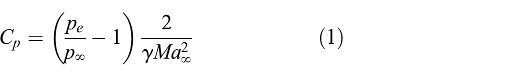
where

Here,
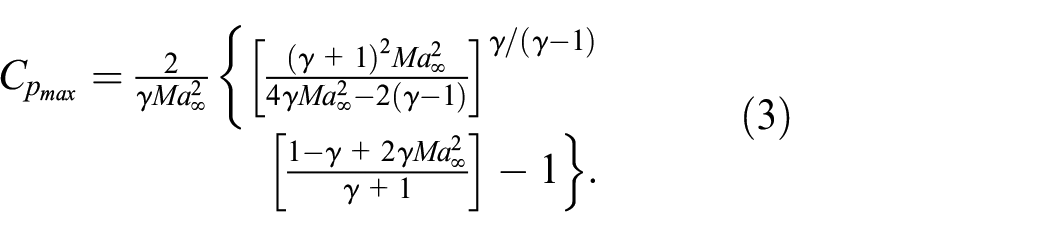
The pressure coefficient on the leeward side is calculated using the Prandtl-Meyer formula, 17 given by

In the above equations,

where
Other gas properties
Once the pressure distribution on the surface has been obtained, additional thermodynamic parameters on the edge of the boundary layer can be determined by combining assumptions of isentropic flow and a gas model (used for non-perfect gases).
In case of a perfect gas, it becomes necessary to compute various parameters including post-bow shock values such as gas pressure


The parameter
However, determining the precise local shock wave angle on the surface is challenging. In engineering estimations for blunt bodies, it is common to assume a value of


where
Equation (9) is derived from the relationship between total pressure and static pressure for an isentropic gas, while equation (10) represents the relationship between Mach number and velocity for a perfect gas. Additionally, the viscosity coefficient
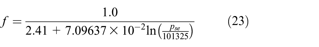
For high temperature chemically equilibrium gases, the following group of fitting formulas of thermodynamic and transport parameters are employed. 18 The entropy can be calculated by
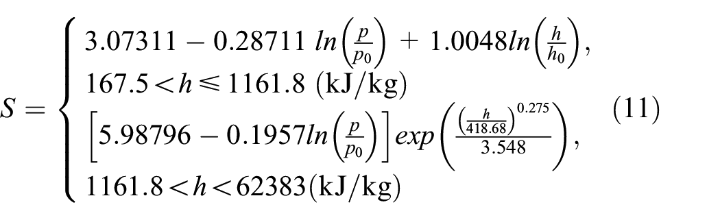
where
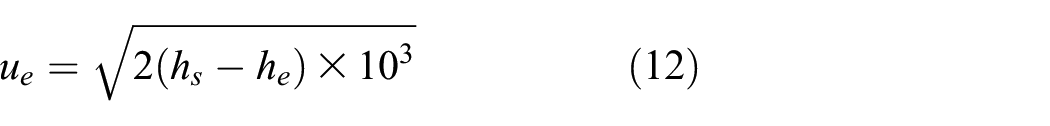
where the enthalpy of stagnation


Temperature


The dynamic viscosity


The local speed of sound

where
Approximate method for heating rate
Heating rate in stagnation region
Assuming that the maximum and minimum radius of principal curvature at a stagnation point on the three-dimensional surface are

where
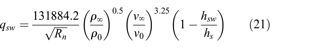
where

In equation (20), the calculation of heating rate requires the radius of curvature at the stagnation point. However, determining the curvature radius at different angles of attack and for various configurations can be challenging for surfaces defined by triangular grids. To address this issue, a quadratic surface is fitted as an approximation to a subset of nodes surrounding the stagnation point. The primary curvature at the stagnation point is estimated by utilizing the primary curvature at the point closest to the stagnation point on the fitted quadratic surface. The quadratic surface is fitted using an equation

where
Kindlmann’s method
21
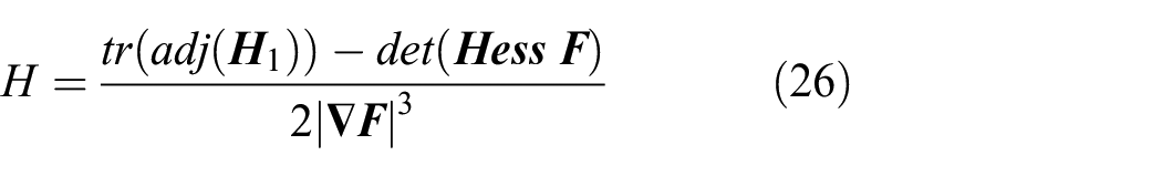
can be utilized to calculate the principal curvatures at a specific point on the quadratic surface determined. To apply this method, begin by determining the Hessian matrix
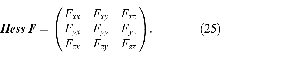
Here,

where


Then, the primary curvatures on the quadratic surface

Once the heating rate at the stagnation point and in the downstream region is obtained, the heating rate on the elements of the stagnation region, excluding the stagnation element, can be calculated through interpolation.
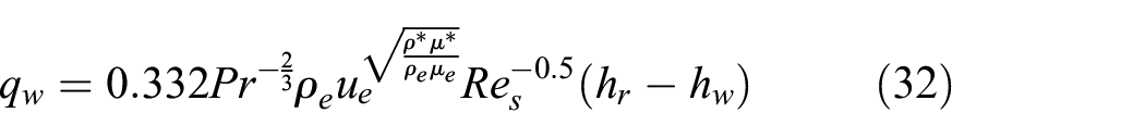
Heating rate in downstream region
Convective heat transfer calculations in high velocity flows typically depend on Eckert’s reference enthalpy theory.
11
The reference enthalpy

where
and for turbulent flows

Here,

Inviscid surface streamlines
Determining the local Reynolds number on the aircraft’s surface is typically necessary to calculate convective heat transfer in high enthalpy flows. The local Reynolds number, defined as

is calculated by integrating along a given streamline starting from the stagnation point, with

where

Direction of velocity on the surface element.

The process of streamlines tracing using two different methods on a double ellipsoid model: (a) points along streamline located on the edges and (b) points along streamline located at the centroid.
However, the process of streamline tracing may encounter special cases where conflicting directions occur at element boundaries and streamline directions at element nodes,
26
as illustrated in Figure 3. This complexity adds challenges to the programming aspect. Moreover, the parameters related to the density

Special cases in streamline tracing: (a) conflicting directions at element boundaries and (b) streamline direction at element node.

Determination method of upstream surface elements.
Figure 5 illustrates the CPU time consumed by both the simplified stream tracing method and the traditional stream tracing method for computing streamlines over the surface of a double ellipsoid at a 0-degree angle of attack, using seven different grid configurations. The computations were conducted on an Intel Core i7-9750H CPU utilizing a single thread. The results indicate that as the number of grids increases, both methods experience an increase in computation time; however, the rate of increase for the simplified stream tracing method is significantly lower than that of the traditional method. This results in approximately a 90% enhancement in computational speed compared to the traditional approach, with the improvement becoming more pronounced as the grid resolution increases. Therefore, when the number of grids is substantial and the computational task is heavy, the time savings offered by the simplified stream tracing method can be considerable.

The performance of the two streamline tracing methods across different grid resolutions.
However, the local Reynolds number computed based on streamlines obtained through this simplified method is susceptible to influence from the surface mesh. Figure 6(a) demonstrates that an inhomogeneous, low-density mesh results in a less smooth computed local Reynolds number. However, increasing the mesh density to reduce non-smoothness comes at the cost of significantly increased computation time, contradicting the purpose of this engineering research.

Effect of filtering on local Reynolds number of OV model: (a) without filter and (b) with filter.
To smooth the local Reynolds numbers on the surface, a mean filter was implemented in this study. The mean filter is a widely used and straightforward technique in image processing. 29 As shown in Figure 7(a), a 3 × 3 filter is illustrated, which replaces the value at the filter’s center with the average of the values within the 3 × 3 surrounding units, where each unit has a weight of 1/(3 × 3). To apply the mean filter to the surface triangular mesh, this study uses neighboring triangular elements as the region over which the mean filter averages values. This neighborhood can consist of elements that share common vertices with the central element, as illustrated in Figure 7(b). When the mean filter traverses and acts on every element on the surface, a complete mean filtering of the surface is achieved. The degree of smoothing by the mean filter can be adjusted by iterating the filtering process multiple times, modifying the weight of the central element, or altering the size of the filter. As shown in Figure 7(c), the neighborhood of the central element includes two layers of neighboring elements, with the second layer composed of elements sharing common vertices with the first layer. The size of the filter, and thus the degree of smoothing, can be controlled by varying the number of these layers. Additionally, to preserve important features during filtering, the filtering region typically avoids areas with abrupt changes or stationary points on the surface. Figure 6(b) illustrates the Reynolds number contour of the OV model after two of mean filtering using the filter shown in Figure 7(b). It is evident that the contour is significantly smoother than before filtering.

Different mean filters: (a) the mean filter for image processing, (b) the mean filter applied to triangular surface meshes, and (c) the larger-sized mean filter applied to triangular surface meshes.
Flow of the aerodynamic heating calculation program
The aerodynamic heating calculation program used in this study comprises three main steps: input, calculation, and output, as illustrated in the flowchart in Figure 8. The input is divided into two parts: one consists of the necessary physical calculation conditions and calculation settings for the computations. The physical calculation conditions include the free-stream Mach number
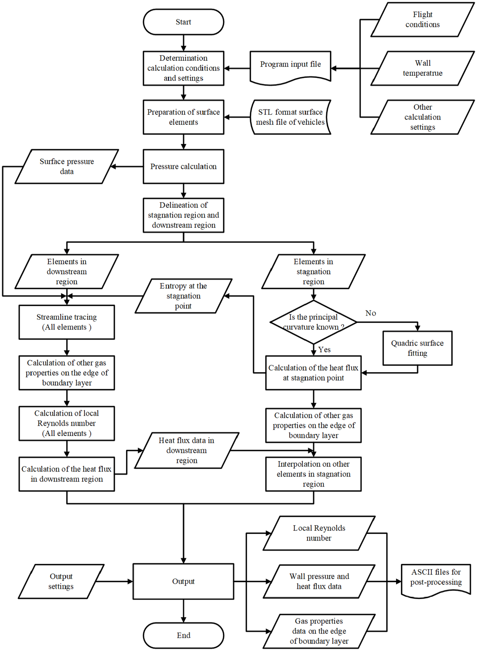
Program calculation process.
After completing the surface pressure calculations, the program will open two threads to calculate the gas parameters on the edge of boundary layer and wall heat flux for both the stagnation region and the downstream region, thereby improving computational efficiency. However, in the threading for calculating heat flux in the downstream region, to ensure the completeness of the output data, streamline tracing and local Reynolds number calculations will also be conducted for the stagnation region units, even though local Reynolds number is not required for the stagnation region heat flux calculations. Once the wall heat flux calculations are completed, the program will export the calculated data in the specified format according to the output settings and provide it to post-processing software.
Examples and results
Example 1: Spherically blunted cone
The spherically blunted model and its wind tunnel experiment data are sourced from the NASA TN D-5450 report. 30 The geometric dimensions of model selected for this study, along with the grid used for the calculations, are shown in Figure 9. The Mesh refinement is applied near the nose of model. The calculation conditions for the calculations are listed in Table 1. When calculating the Reynolds number, the mean filter shown in Figure 7(a) was applied iteratively twice to the local Reynolds number for smoothing. The angle parameter for adjusting the stagnation region was set to 1.5°.
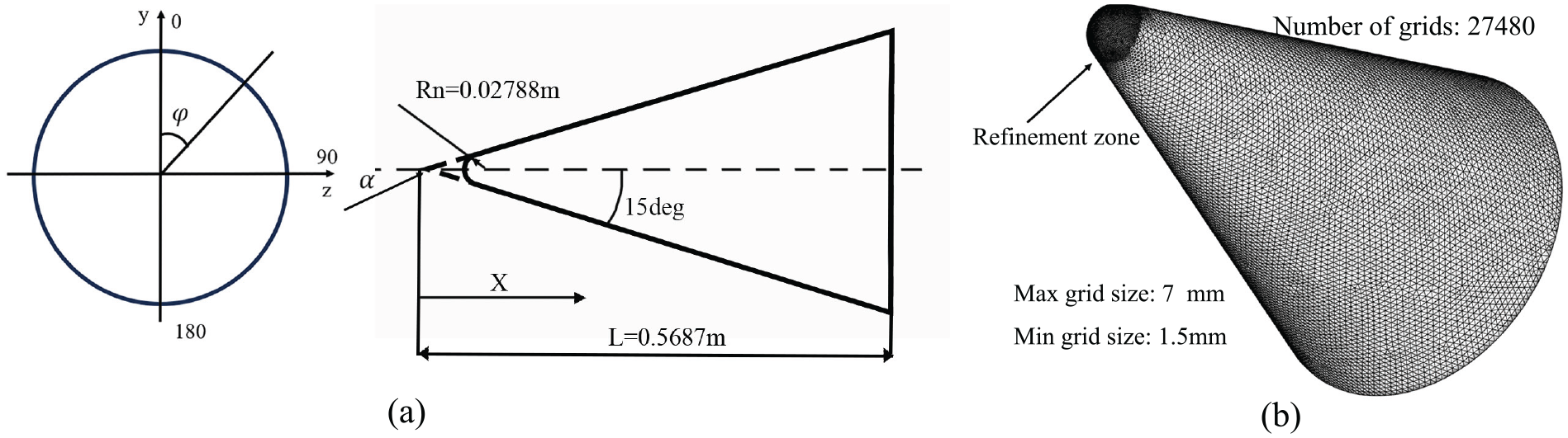
The spherically blunted cone model: (a) geometry of the spherically blunted cone and (b) the surface mesh of the spherically blunted cone.
The calculation conditions for heating prediction of the spherically blunted cone.

Figure 10 illustrates the heat flux along the centerline of different cross-sections at angles

The heat flux along the centerline of different cross-sections under conditions 1 and 2: (a) condition 1, AOA 0,
Figure 11 presents the heat flux contours calculated using a chemical equilibrium gas model. It can be observed that in operating conditions 1 and 2, the wall heat flux in the downstream region is relatively stable, indicating laminar flow. However, as the incoming Mach number increases, conditions 3 and 4 exhibit a abrupt rise in wall heat flux in the downstream area, with the flow transition being the primary cause of this abrupt change. As illustrated, the transition points in conditions 3 and 4 occur at nearly the same location, and the wall heat flux in the turbulent regime is approximately four times greater than that in the laminar regime. Figure 12 shows that the laminar heat flux in condition 4 is approximately 40% higher than in condition 3, while the wall heat flux in the turbulent region is approximately 60% greater. This indicates that as the Mach number increases, the rate of heat flux growth in turbulent flow typically surpasses that in laminar flow.

Heat flux contours of the spherically blunted cone under different calculating conditions (chemical equilibrium gas model): (a) AOA 0,

The heat flux along the centerline of the windward surface at different Mach numbers.
Figure 13 illustrates the CPU time consumption of two gas models during two calculation processes related to the gas models under varying grid densities. The figure reveals that the primary difference in computation time between the two models occurs in the calculation of gas parameters at the boundary layer edge. The chemical equilibrium gas model requires methods such as bisection or other iterative approaches to determine certain gas parameters, while the perfect gas model allows for direct computation. This difference is the main reason for the observed time discrepancies. Compared to the chemical equilibrium gas model, the perfect gas model can save 70%–75% of the time in computing gas parameters at the boundary layer edge and reduce the time for heat flux calculations in the downstream region by 5%–20%, resulting in an overall time reduction of 65%–70% for these two processes combined.

Performance of the two gas models in gas model-related calculation processes under different grid resolutions.
Example 2: OV model
The Orbiter Vehicle (OV) model is derived from Greene et al. 31 The dimensions of the model and the grid used for calculations are shown in Figure 14, while Table 2 presents the freestream conditions used for calculations. In calculating the local Reynolds number, a mean filter from Figure 7(b) was applied iteratively twice to smooth the Reynolds number, with an angular parameter set to 0.5° to adjust the size of the stagnation region.

The OV model: (a) the geometry of OV model and (b) the surface mesh of OV model.
The calculation conditions for heating prediction of OV model.

Figure 15 illustrates the heat flux contours of the OV model under conditions 1 and 2, calculated with two different gas models. The heat flux peak area around the stagnation point is larger when the chemical equilibrium gas model is used than when the perfect gas model is applied. The gas temperature around the stagnation point is generally higher, which may result in air dissociation. Consequently, the perfect gas model might fail to accurately predict the gas properties at the boundary layer edge, leading to a gradient of heat flux along the streamwise direction over relatively smooth surfaces. In contrast, the calculations using the chemical equilibrium gas model appear to better align with the actual physical situation.

Heat flux contours of the OV model under different calculating conditions: (a) condition 1, perfect gas model, (b) condition 1, chemical equilibrium model, (c) condition 2, perfect gas model, and (d) condition 2, chemical equilibrium model.
Additionally, Figure 15 reveals that aside from the peak heat flux area at the stagnation point, a crescent-shaped peak heat flux region also forms at the edge of the OV model’s nose. The heat flux in this region is comparable to the stagnation heat flux under calculation condition 1. When the angle of attack increases to 18°, the extent of the peak heat flux region slightly decreases, although the wall heat flux experiences a significant increase. The rapid increase in gas velocity along the streamline direction at the model’s nose edge is likely the direct cause of this peak heat flux region. As shown in Figure 16(a), the pressure coefficient contours for calculation condition 1 indicate that gas pressure rapidly decreases along the streamline direction at the windward surface’s edge, suggesting that the gas is undergoing rapid expansion in this region. This leads to substantial increases in gas velocity, as illustrated in Figure 16(b). Although the gas enthalpy and density decrease, they remain relatively high compared to the leeward surface’s nose edge due to proximity to the stagnation point, as shown in Figure 16(c) and (d). Gas acceleration under higher enthalpy and density conditions contributes more significantly to the wall heat flux than under lower enthalpy and density conditions. Therefore, the peak heat flux occurs at the windward surface’s nose edge, but not at the corresponding edge on the leeward side.

Gas parameters at the edge of the boundary layer on the OV model under condition 1: (a) pressure coefficient contours, (b) the velocity at the edge of boundary layer along the centerline, (c) the density at the edge of boundary layer along the centerline, and (d) the enthalpy at the edge of boundary layer along the centerline.
Figure 17 presents the dimensionless heat flux along the centerline of the windward surface under conditions 1 and 2, with experimental data sourced from Greene et al. 31 It is clear that the heat flux in the cylindrical section of the model closely matches the experimental measurements for both conditions, with a relative error of less than 15%. However, significant discrepancies are observed in the downstream expansion section of the OV model under both conditions. For condition 2, Greene et al. 31 indicates that flow transitions occurred in the downstream expansion section; however, the transition criterion used in this study failed to accurately predict the transition, which may be a primary reason for the observed errors.

Dimensionless heat flux along the centerline of the windward side of the OV model: (a) condition 1 and (b) condition 2.
Additionally, in the surface extension section of the downstream region, a substantial amount of inviscid flow mass is entrained into the boundary layer. The surface streamlines originating from the stagnation region are engulfed by the boundary layer, leading to a disparity between the entropy at the boundary layer edge and the entropy at the stagnation point. This disparity could be one potential explanation for the observed discrepancies, as the computational method assumed in this paper may not be applicable in such scenarios.
Conclusion
This paper provides a detailed and comprehensive introduction to the aerodynamic heating calculation engineering method for hypersonic blunt body vehicles. By simplifying the streamline tracing approach, the paper enhances computational efficiency while validating the effectiveness of the engineering method through two examples. The conclusions drawn from this research are as follows:
The simplified streamline tracing method constructed in this study effectively enhances computational efficiency, achieving a 90% reduction in the time required for streamline calculations compared to traditional methods.
Validation results using a spherically blunted cone and OV models indicate that the method effectively predicts wall heat flux for blunt-body vehicles at small angles of attack. In the stagnation and non-expanded downstream regions, the method achieves a relative error of less than 15%.
In downstream expansion regions and at high angles of attack, the method shows larger errors in wall heat flux prediction. Incorporating a more accurate flow transition criterion and applying entropy corrections may help reduce these errors.
While the difference between results obtained using a perfect gas model and those from a chemical equilibrium gas model is generally small, using the perfect gas model can reduce computational time by 65%–70%. For most conditions, the perfect gas model is appropriate; however, for high-enthalpy flows and regions near stagnation points, the chemical equilibrium gas model provides more reasonable results.
In conclusion, the method presented in this paper strikes a practical balance between accuracy and efficiency, making it well-suited for the engineering design of hypersonic vehicles, particularly during the early design stages.
Footnotes
Handling Editor: Sharmili Pandian
Funding
The author(s) disclosed receipt of the following financial support for the research, authorship, and/or publication of this article: National Natural Science Foundation of China (Grant: 12362026 and 11862017).
Declaration of conflicting interests
The author(s) declared no potential conflicts of interest with respect to the research, authorship, and/or publication of this article.