Sage Journals: Discover world-class research

Abstract

In practical industrial applications, the operating conditions of bearings frequently change, posing significant challenges for reliable fault diagnosis. Traditional machine learning methods, which rely on the assumption of independent and identically distributed samples, often experience a significant decline in diagnostic accuracy under such variable conditions. To address this issue, this paper proposes a bearing fault transfer diagnosis method that combines the Balanced Distribution Adaptation (BDA) algorithm with a Back Propagation neural network (BPNN) classification algorithm. Firstly, time-domain features of the bearing signals are extracted to comprehensively reflect the operational state of the bearings. Principal Component Analysis (PCA) is then utilized to reduce the dimensionality of the high-dimensional features, preserving the main information while reducing computational complexity. Subsequently, the BDA algorithm is employed to align the features of the source and target domains, balancing distribution differences and achieving effective feature space transfer. Finally, the BP neural network classification algorithm is used to classify the transferred features, thereby diagnosing bearing faults. Experimental results demonstrate that, compared to traditional fault diagnosis methods, the proposed approach achieves higher diagnostic accuracy and robustness under different working conditions. This method not only addresses the challenges posed by changing operating conditions but also holds significant practical value, providing a robust and efficient solution for real-world industrial applications such as predictive maintenance and condition monitoring in critical engineering systems.

Keywords

balanced distribution adaptive back propagation neural network (BPNN)bearing fault diagnosis feature migration principal component analysis

Introduction

Bearings, as critical components in mechanical equipment, directly influence the overall system’s operational state and lifespan.¹ Therefore, timely and effective bearing fault diagnosis is essential for preventing equipment failures, reducing downtime, and lowering maintenance costs. Traditional bearing fault diagnosis methods primarily rely on expert knowledge and experience. However, these methods often struggle to adapt to complex and variable working conditions.² With advancements in computational technology and data acquisition techniques, data-driven machine learning methods have been widely applied in bearing fault diagnosis, demonstrating excellent diagnostic performance.

Nevertheless, most traditional machine learning methods assume that the training and testing data are independently and identically distributed, which is often not the case in practical applications.³ In real industrial environments, bearing operating conditions, such as load, speed, and ambient temperature, frequently change, leading to significant differences between the training and testing data distributions. This distribution discrepancy significantly degrades the diagnostic performance of traditional machine learning methods under varying conditions.⁴ Thus, maintaining high diagnostic accuracy and efficiency under variable conditions has become a current research hotspot and challenge.

Additionally, a number of researchers have explored the combination of statistical signal processing with intelligent algorithms to mitigate the effects of non-stationary operating conditions.⁵ Techniques such as wavelet transforms,⁶ empirical mode decomposition,⁷ and time-frequency analysis have been applied to extract robust features from vibration signals under diverse conditions.⁸ These feature extraction methods, when paired with classifiers like support vector machines and neural networks, have demonstrated improved fault diagnosis performance. However, challenges related to data scarcity and model generalization under changing conditions still persist, indicating a clear research gap.

More recent research has focused on transfer learning⁹ and domain adaptation as promising approaches to address the discrepancy between training and testing data distributions in variable industrial settings, including adaptive algorithms and shared feature space construction, have been developed to minimize the differences between source, and target domains. These innovative strategies enhance the robustness and accuracy of fault diagnosis systems, providing a comprehensive framework that addresses both the theoretical and practical challenges of bearing fault diagnosis in real-world applications.

Recent advancements in transfer learning have significantly impacted the field of bearing fault diagnosis. Traditional machine learning methods often struggle under varying industrial conditions due to the assumption of identical data distributions between training and testing datasets. In contrast, transfer learning techniques leverage labeled data from a source domain to enhance the performance of models in a target domain where data distributions may differ markedly. Researchers have explored various strategies such as Maximum Mean Discrepancy (MMD)¹⁰ and adversarial domain adaptation networks (AAN) to align the feature spaces of disparate domains, thereby mitigating the adverse effects of domain shifts. Additionally, novel approaches incorporating adaptive weighting and balanced distribution adaptation have been developed to handle the imbalance between intra-class and inter-class distributions, further refining the discriminative power of the extracted features.

However, earlier methods like Transfer Component Analysis (TCA)¹¹ and Joint Distribution Adaptation (JDA)¹² exhibit certain limitations. TCA primarily focuses on aligning the marginal distributions of source and target data, often neglecting the conditional distributions, which can be critical for accurate fault diagnosis. JDA attempts to address this by aligning both marginal and conditional distributions, but it may struggle with balancing the trade-off between these two aspects, potentially compromising the diagnostic performance under highly variable conditions. However, the Balanced Distribution Adaptation (BDA) algorithm, which offers a more nuanced approach by adaptively weighting and balancing the distribution discrepancies, thereby achieving superior alignment and improved fault diagnosis outcomes.

This paper proposes a bearing fault transfer diagnosis method that combines the Balanced Distribution Adaptation (BDA) algorithm with the Backpropagation Neural Network (BPNN) classification algorithm. This method achieves bearing fault diagnosis through the following main steps: (1) Extracting rich time-domain features from bearing vibration signals to comprehensively reflect the bearing’s operational state. Time-domain features include metrics that describe the statistical properties of the signals, such as mean, variance, skewness, and kurtosis. (2) Using Principal Component Analysis (PCA) to reduce the dimensionality of the high-dimensional features. PCA linearly transforms the original high-dimensional features into a low-dimensional space, retaining the primary feature information while reducing data redundancy and computational complexity, thus enhancing feature processing efficiency. (3) Applying the Balanced Distribution Adaptation algorithm to align the features of the source and target domains. The BDA algorithm introduces an adaptive weighting strategy in the feature space to adjust the distribution of the source and target domain data, making them more consistent in the new feature space, thereby effectively reducing the discrepancy between the feature distributions of the source, and target domains. (4) Combining the Backpropagation Neural Network classification algorithm to classify the transferred features. The BP neural network adjusts weights through the backpropagation algorithm to minimize prediction errors, thereby improving classification accuracy and robustness. BP neural networks excel at handling complex nonlinear problems, making them suitable for bearing fault diagnosis tasks.

Materials and methods

Feature extraction

In vibration signal analysis, time-domain feature extraction is crucial.¹³ The vibration signals generated during the operation of rotor systems contain rich fault information. By performing statistical analysis on the time-domain signals, various feature parameters can be extracted that reflect the overall trend, fluctuation level, and subtle changes of the signals, aiding in the diagnosis of different types of faults.^14,15 Below are the commonly used time-domain features and their physical meanings, as shown in Table 1.

Table 1.

Expressions of different time-domain features.

Time-domain features	Expressions
Mean	$Mean = \frac{1}{N} \sum_{i = 1}^{N} x_{i}$
Root mean square	$RMS = \sqrt{\frac{1}{N} \sum_{i = 1}^{N} x_{i}^{2}}$
Variance	$Va = \frac{1}{N} \sum_{i = 1}^{N} {(x_{i} - μ)}^{2}$
Peak value	$P = max (\| x_{i} \|)$
Crest factor	$C = \frac{P}{RMS}$
Skewness	$S = \frac{1}{N} \sum_{i = 1}^{N} {(\frac{x_{i} - μ}{σ})}^{3}$
Kurtosis	$K = \frac{1}{N} \sum_{i = 1}^{N} {(\frac{x_{i} - μ}{σ})}^{4}$
Clearance factor	$M = \frac{P}{\frac{1}{N} \sum_{i = 1}^{N} \| x_{i} \|}$
Shape factor	$F = \frac{RMS}{\frac{1}{N} \sum_{i = 1}^{N} \| x_{i} \|}$
Impulse factor	$I = \frac{P}{\frac{1}{N} \sum_{i = 1}^{N} \| x_{i} \|}$

In this study, MATLAB was employed to implement the feature extraction process. This section focuses on several selected time-domain indicators due to their effectiveness and low computational complexity. MATLAB enabled efficient processing of vibration data to compute features such as mean, RMS, standard deviation, skewness, kurtosis, and others, forming an initial high-dimensional feature set that captures the system’s fault characteristics.

The time-domain features of bearing vibration signals reveal key physical characteristics. The mean indicates the average level and DC component, while the RMS value quantifies signal energy, with higher values suggesting greater energy. Variance reflects the signal’s dispersion, and the peak value identifies maximum amplitudes, highlighting impact events. The crest factor (peak-to-RMS ratio) is particularly sensitive to impact faults. Skewness and kurtosis provide insights into the distribution’s symmetry and sharpness, respectively, with high kurtosis often indicating strong impacts. Additionally, the clearance, shape, and impulse factors describe the waveform’s morphology and the intensity of impact components.¹⁶ Collectively, these features offer a comprehensive view of the vibration signal’s statistical properties, which is essential for effective rotor fault diagnosis.

Principal component analysis (PCA) dimensionality reduction algorithm

Principal Component Analysis (PCA) is a widely used unsupervised learning algorithm for dimensionality reduction and feature extraction. Its goal is to project high-dimensional data onto a lower-dimensional space through linear transformation while preserving as much of the data’s variance as possible. Specifically, PCA aims to identify the principal components of the data, which are the directions that explain the most variance in the data.^17–19 These principal components are linear combinations of the original features, capturing the maximum variance information in the new coordinate system. The main steps of PCA are as follows:

(1) The original data is centered by subtracting the mean to eliminate the effect of data translation.

(2) Covariance matrix calculation: The covariance matrix of the data is computed. Suppose there is an N×D data matrix X, where N is the number of samples and D is the feature dimension. The formula for the covariance matrix is as follows:

\sum = \frac{1}{N} (X - \bar{X})^{T} (X - \bar{X})

(1)

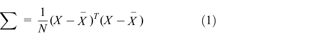
Where, $\bar{X}$ is the mean vector of the data.

(3) Perform eigenvalue decomposition on the covariance matrix to obtain eigenvalues $λ_{1}, λ_{2}, \dots λ_{D}$ and their corresponding eigenvectors $v_{1}, v_{2}, \dots, v_{D}$ .

(4) Based on the magnitude of the eigenvalues, select the top K eigenvectors to form the projection matrix W. Typically, the top K eigenvectors with the largest variances are chosen as principal components.

(5) Multiply the original data matrix X by the projection matrix W to obtain the reduced-dimensional data matrix Z. The projection is formulated as follows:

Z = XW

(2)

Given a dataset X, where each sample $x_{i}$ is a D-dimensional vector, PCA aims to find a projection matrix W of dimension $K < D$ such that the data X projected into the K-dimensional space maximizes the variance of the samples. The optimization objective of PCA can be formulated as maximizing the total variance of the projected data. This is achieved by finding a projection matrix W that maximizes the trace of the covariance matrix of the projected data. The maximization objective function can be expressed as follows:

max_{W} Tr (W^{T} \sum W)

(3)

Where, $Σ$ is the covariance matrix of the original data.

Following the steps of PCA as described above effectively reduces feature dimensions, eliminates redundant information, and enhances the accuracy and reliability of fault feature extraction. This provides superior input features for subsequent machine learning models, thereby improving the performance of fault diagnosis.

Balanced distribution adaptation (BDA) algorithm

The Balanced Distribution Adaptation (BDA) algorithm is a transfer learning method designed to address the issue of disparate data distributions between source and target domains.²⁰ Its core idea involves introducing adaptive weighting strategies in the feature space to adjust the distributions of source and target domain data, thereby aligning them in the new feature space.²¹

Algorithm steps

(1) Constructing Initial Classifier: Train an initial classifier on the source domain data. Typically, a linear classifier such as Support Vector Machine (SVM) or Logistic Regression is used. The classifier can be represented as $f (x) = sign (w^{T} x + b)$ , where w is the weight vector and b is the bias term.

(2) Computing Weighting Matrix: Based on the distribution differences between the source and target domain data, compute a weighting matrix W to adjust the weights of the source and target domain data. The computation of the weighting matrix can utilize methods such as kernel density estimation to quantify the distribution disparities between the two domains. Assuming the source and target domain data are denoted as Xs and Xt, respectively, the computation of the weighting matrix can be expressed as:

W_{ij} = \exp (- \frac{{‖ {x_{i}}^{T} - {x_{j}}^{S} ‖}^{2}}{2 σ^{2}})

(4)

Where, ${x_{i}}^{T}$ is the i-th sample from the target domain data, ${x_{j}}^{S}$ is the j-th sample from the source domain data, and $σ$ is the bandwidth parameter of the kernel function.

(3) Optimization Objective Function: By minimizing the objective function, adjust the parameters of the classifier to minimize classification errors on the target domain. Typically, optimization algorithms such as gradient descent are used to optimize the objective function. The objective function for optimization can be represented as:

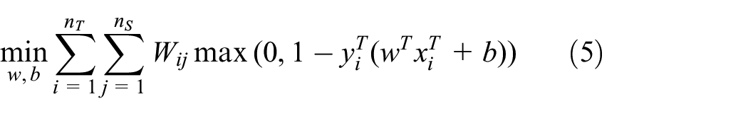
min_{w, b} \sum_{i = 1}^{n_{T}} \sum_{j = 1}^{n_{S}} W_{ij} max (0, 1 - y_{i}^{T} (w^{T} x_{i}^{T} + b))

(5)

Where, $y_{i}^{T}$ is the true label of the i-th sample from the target domain data.

(4) Iterative Updating: Iteratively update the weighting matrix and classifier parameters until convergence criteria are met. During each iteration, based on the current weighting matrix and classifier parameters, recalculate the objective function and update the parameters accordingly.

Mathematical expression of the algorithm

Given the source domain dataset $X_{s}$ and target domain dataset $X_{t}$ , along with their corresponding labels $y_{s}$ and $y_{t}$ , the goal of BDA is to learn a mapping function f that minimizes the prediction error on the target domain. The optimization objective can be expressed as minimizing a loss function that considers the distribution differences between the source and target domain data. The mathematical expression is given as follows²²:

min_{f} \sum_{i = 1}^{n_{T}} W_{ij} L (f (x_{i}^{T}), y_{j}^{S})

(6)

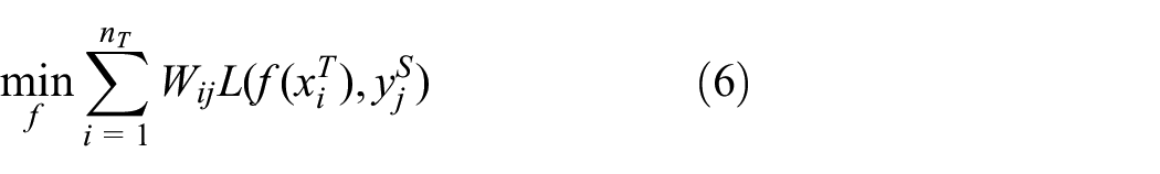
Where L is the loss function, and $W_{ij}$ is the sample weight, which measures the adaptability of the source domain sample $x_{j}^{S}$ to the target domain sample $x_{t} (i)$ . The BDA algorithm iteratively optimizes the objective function by continuously adjusting the weighting matrix W and the classifier parameters, thereby achieving adaptive weighting of the source and target domain data to enhance classification performance in the target domain.

Back propagation neural network (BPNN)

The Back Propagation Neural Network (BPNN) is a commonly used artificial neural network model widely applied in fields such as pattern recognition, classification, and regression. BPNN adjusts the network weights and biases through the backpropagation algorithm to achieve effective mapping of input data.^23,24 It typically consists of the following components:

(1) Input Layer: Receives the input data, with each node corresponding to an input feature.

(2) Hidden Layer: Positioned between the input and output layers, it can contain one or more hidden layers, each comprising several neurons. The number of hidden layers and neurons per layer are hyperparameters of the network that need to be adjusted based on the specific problem.

(3) Output Layer: Produces the output results, with the number of nodes corresponding to the output dimensions.

The network structure is illustrated in Figure 1.

Figure 1.

Network architecture diagram of the BP neural network.

During the forward propagation process, input data sequentially passes through the input layer, hidden layers, and output layer. The weighted sum and bias for each neuron in every layer are calculated, and the output is obtained through an activation function.

The input and output calculations for the j-th neuron in the hidden layer are as follows:

z_{j} = \sum_{i = 1}^{n} w_{ij} x_{i} + b_{j}

(7)

Where, $w_{ij}$ is the weight connecting the i-th input neuron to the j-th hidden neuron, $b_{j}$ is bias term for the j-th hidden neuron, $z_{j}$ is weighted sum (pre-activation) of the j-th hidden neuron.

a_{j} = f (z_{j})

(8)

The input and output calculations for the output layer are as follows:

z_{k}' = \sum_{j = 1}^{m} w_{jk}' a_{j} + b_{k}'

(9)

y_{k}' = f (z_{k}')

(10)

The BP neural network is a neural network model that adjusts network weights and biases using the backpropagation algorithm to minimize the error function E. During the forward propagation process, input data sequentially passes through the input layer, hidden layers, and output layer, computing the weighted sum and bias of each layer’s neurons, and obtaining outputs through activation functions. The BP neural network utilizes the Mean Squared Error (MSE) as the error function:

E = \frac{1}{2} \sum_{k = 1}^{p} {(y_{k}' - y_{k})}^{2}

(11)

Where, $y_{k}'$ is target (true) value for the k-th output neuron, $y_{k}$ is predicted output of the k-th output neuron.

During the backpropagation process, the first step is to compute the error at the output layer.

δ_{k} = (y_{k}' - y_{k}) f' ({z'}_{k})

(12)

Where, $δ_{k}$ is error term for the k-th output neuron, $f'$ is derivative of the activation function.

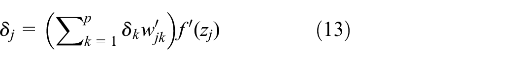
Then compute the error at the hidden layer.

δ_{j} = (\sum_{k = 1}^{p} δ_{k} w_{jk}') f' (z_{j})

(13)

Finally, update the weights and biases using gradient descent.

w_{jk}' \leftarrow w_{jk}' - η δ_{k} a_{j}

(14)

b_{k}' \leftarrow b_{k}' - η δ_{k}

(15)

Where, η represents the learning rate. The commonly used activation functions include the Sigmoid function, Tanh function, and ReLU function, which introduce nonlinearity to enable the network to handle complex nonlinear problems.

BDA-BPNN for bearing fault feature transfer diagnosis

In order to validate the effectiveness of the BDA algorithm in bearing fault transfer diagnosis under variable operating conditions, this study designed cross-platform validation experiments. These experiments encompass two types, each representing different data sources and working environments, thus comprehensively assessing the applicability, and robustness of the BDA algorithm. Two distinct datasets were selected for experimentation: one sourced from publicly available bearing datasets abroad, and another collected from laboratory test rig bearing datasets. These datasets represent bearing operational data from diverse sources and characteristics, covering a range of operating conditions. Through these experiments, the diagnostic performance of the BDA algorithm across different operating conditions will be thoroughly evaluated, providing reliable reference for practical applications. Figure 2 The specific flowchart is as follows:

Figure 2.

Process diagram for bearing fault feature transfer diagnosis using BDA-BPNN.

Experimental validation and analysis

Experimental design

To validate the effectiveness of the BDA algorithm in bearing fault transfer diagnosis under varying operating conditions, this study conducted experiments across different platforms and operating conditions to comprehensively assess the algorithm’s applicability and robustness. Two distinct datasets were utilized to ensure the algorithm’s effectiveness and robustness under various operational conditions. One dataset was sourced from the publicly available bearing data repository of Case Western Reserve University (CWRU), USA. This database includes bearing data collected under diverse operating conditions, meticulously designed and curated to cover various typical bearing fault types such as inner race faults, outer race faults, and rolling element faults. Each operational condition’s dataset comprises rich vibration signals, ensuring high representativeness and reliability. The experimental setup for this dataset is illustrated in Figure 3.

Figure 3.

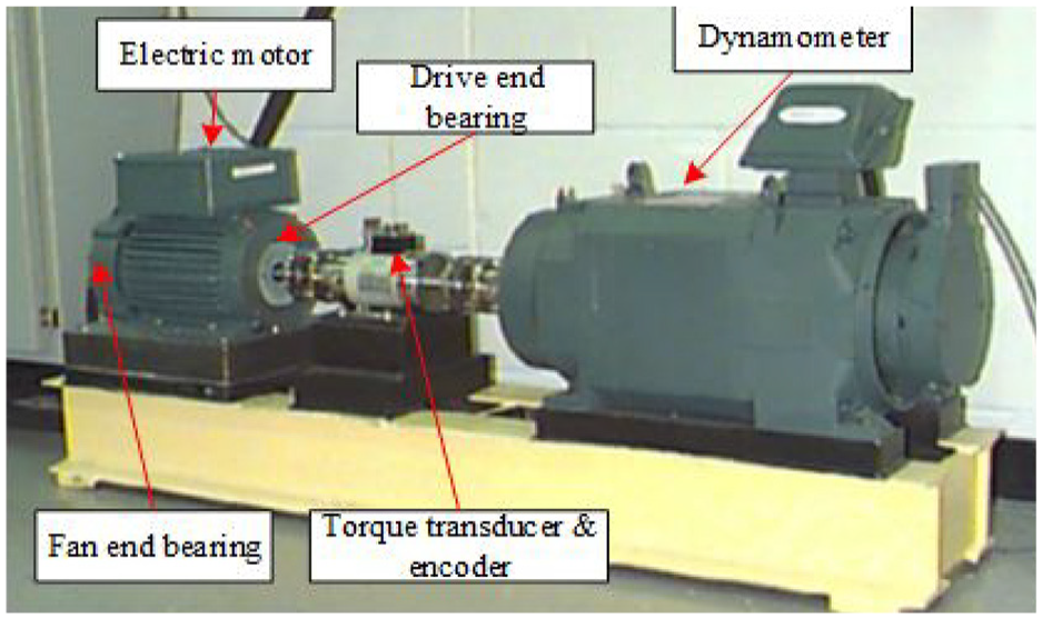
Case western reserve university bearing fault test rig.

The other dataset was obtained from a laboratory-built test rig designed to simulate real-world bearing operating environments. Data from the laboratory test rig encompass vibration signals collected under different loads, speeds, and environmental conditions. By precisely controlling experimental parameters, the laboratory test rig simulates multiple real-world conditions to capture bearing data under different states. The dataset includes vibration signals not only from normal operating conditions but also from fault conditions such as wear or damage to the inner race, outer race, and rolling elements. The experimental device of the laboratory test bench and the simulated fault signal diagram are shown in Figures 4 and 5 respectively.

Figure 4.

Laboratory WS-ZHT1-2 type bearing fault test rig.

Figure 5.

The simulated fault signal diagram. (a) Rotor vertical fault diagram. (b) Rotor misalignment fault diagram. (c) Rotor unbalance fault diagram. (d) Rotor horizontal deviation fault diagram.

Besides the operating conditions described in Table 2, the CWRU dataset also includes conditions with rotational speeds of 1797 and 1750 r/min, facilitating subsequent experimental research.

Table 2.

Parameter data of different bearing sample sets.

Dataset	Fault type	Sampling frequency (kHz)	Rotational speed	Fault code
CWRU dataset	Normal	48	1772	0
	Outer race	48	1772	1
	Inner race	48	1772	2
	Rolling element	48	1772	3
Laboratory dataset	Normal	32	800	0
	Outer race	32	800	1
	Inner race	32	800	2
	Rolling element	32	800	3

Dimensionality reduction of signal features

The collected vibration signal data were processed using MATLAB to extract corresponding time-domain features, as detailed in Table 1. These features include mean, root mean square (RMS), kurtosis, skewness, peak value, variance, peak-to-peak value, impulse factor, margin factor, and waveform factor, comprehensively reflecting the statistical properties and trends of the signals. Subsequently, Principal Component Analysis (PCA) was employed to perform dimensionality reduction on all extracted time-domain features.

First, the features were standardized to eliminate the influence of different dimensions and scales among them. The covariance matrix of the feature matrix was then calculated, and eigenvalue decomposition was performed to obtain eigenvalues and eigenvectors. The principal components with the highest cumulative explained variance were selected based on the magnitude of the eigenvalues. In this study, the top five principal components were chosen, and the original features were projected into this principal component space to obtain the reduced-dimensionality features. These features retained most of the information and trends from the original data, making them more effective for subsequent fault diagnosis analysis, thereby improving diagnostic accuracy, and reliability. The explained variance plot of the PCA-reduced features is shown in Figure 6.

Figure 6.

Variance explained of principal components after PCA dimensionality reduction.

Figure 6 shows that after PCA dimensionality reduction, the cumulative contribution rate of the first five principal components exceeds 90%, adequately representing the primary trends, and information content of the original data. These reduced features retain the original information, significantly reduce data redundancy, and effectively distinguish between different fault states. PCA dimensionality reduction greatly reduces the data dimensions and computational complexity, improving model training and prediction efficiency, while enhancing the model’s stability, and generalization capability.

Cross-platform diagnostic verification and analysis

To validate the effectiveness of the proposed balanced domain adaptation (BDA) algorithm, a visual analysis of feature transfer was conducted, comparing the feature distribution before transfer and after transfer using TCA (Transfer Component Analysis), JDA (Joint Distribution Adaptation), and BDA algorithms. The visualization of feature transfer before and after is shown in Figure 6.

As seen in Figure 7(a), before feature transfer, the features of different states are mostly clustered together in the feature space, making it difficult to distinguish between different fault states, and affecting the accuracy of fault diagnosis. Figure 7(b) shows that after processing with the JDA algorithm, the feature distribution improves, but the features of the normal state and rolling element fault state are still mixed. The TCA algorithm further improves feature distribution by aligning the marginal and conditional distributions of the source and target domains, but the issue of confusion between the normal state and the rolling element fault state persists.

Figure 7.

Visualization after different feature transfer algorithm. (a) Visualization before feature transfer. (b) Visualization after JDA feature transfer. (c) Visualization after TCA feature transfer. (d) Visualization after BDA feature transfer.

From Figure 7(d), it is evident that the feature distribution significantly improves after applying the proposed Balanced Distribution Adaptation (BDA) algorithm for feature transfer. By balancing the distribution between the source domain and the target domain, the BDA algorithm effectively optimizes the feature space, resulting in better separation of features under different conditions. After BDA processing, the features of normal and faulty states are clearly separated, without clustering together. This indicates that the BDA algorithm effectively adjusts the data distribution between the source and target domains during feature transfer, enhancing the accuracy and reliability of fault diagnosis. Compared to TCA and JDA algorithms, the BDA algorithm demonstrates stronger generalization ability and robustness in fault diagnosis tasks under complex conditions.

The diagnostic accuracy of various models at different rotational speeds is shown in Table 3. The results indicate that BDA outperforms other transfer learning algorithms in optimizing distribution adaptation, achieving an average diagnostic accuracy of 96%. In contrast, the diagnostic accuracy using the TCA method is about 78%, showing some improvement but still not ideal. The diagnostic accuracy of the JDA method ranges from 82% to 86%. Although it shows significant improvement over TCA, it still falls short of the performance achieved by the BDA algorithm.

Table 3.

Diagnostic accuracy of different models under varying rotational speeds (%).

Classification model	1750 r/min→800 r/min	1772 r/min→800 r/min	1797 r/min→800 r/min
BPNN	42.0	40.6	44.2
TCA-BPNN	78.2	80.8	76.6
JDA-BPNN	86.6	82.2	84.6
BDA-BPNN	97.2	96.8	96.4

In Table 3, the bolded numbers represent the highest accuracy values for each method under the corresponding conditions.

In order to verify the validity of the proposed model, several common diagnostic models such as support vector machine (SVM), K-nearest neighbor algorithm (KNN), decision tree (DT) and radial basis neural network (RBF) are compared, and the results are as follows: The result is shown in Figure 8.

Figure 8.

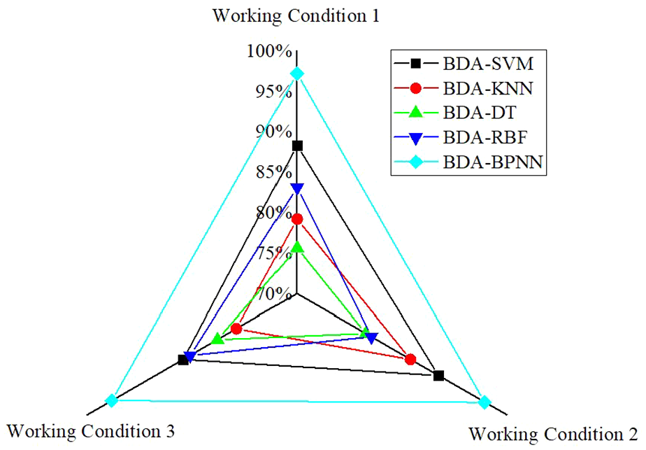
Diagnostic accuracy of different models under feature transfer.

Under the three different working conditions (1750, 1772, and 1797 r/min transferred to 800 r/min), the BDA-BPNN demonstrated exceptional performance. Its accuracy remained above 90% across all conditions, showing strong generalization capabilities, particularly excelling under Working Condition 2 (1772 r/min→800 r/min) where the accuracy reached nearly 100%. This result indicates that BDA-BPNN adapts well to transitions between different high-speed conditions and the low-speed laboratory condition, exhibiting excellent stability and robustness in handling varying working speeds.

Compared to other algorithms like BDA-SVM and BDA-KNN, BDA-BPNN performed significantly better, especially under Working Condition 2, where the performance of other algorithms noticeably declined, while BDA-BPNN maintained nearly perfect accuracy. Its performance was also stable in Working Conditions 1 and 3, effectively handling challenges across different conditions. This demonstrates that BDA-BPNN not only has strong learning abilities in cross-condition transfer learning but also excellent adaptability, making it a highly effective model choice for application under multiple working conditions.

Results

This paper proposes a bearing fault diagnosis method based on the BDA-WKNN approach, and the effectiveness of the proposed method is verified through experiments. The main conclusions are as follows:

(1) To tackle the challenge of uneven sample distribution and varying feature differences caused by different operating conditions and rotational speeds, the Balanced Distribution Adaptation (BDA) algorithm is employed. BDA adaptively aligns the feature distributions between the training and testing data, ensuring that fault-relevant information is consistently captured despite domain discrepancies. Experimental results indicate that this adaptive adjustment effectively reduces misclassification arising from distribution shifts.

(2) To further improve diagnostic accuracy, the method integrates the Weighted K-Nearest Neighbors (WKNN) classifier, which assigns higher weights to samples closer to the query point. This weighted approach enhances the influence of more relevant neighboring samples, thereby boosting the overall decision-making process and classification performance, especially under noisy, or variable conditions. Comparative experiments show that WKNN outperforms traditional KNN, particularly in scenarios with imbalanced or challenging data distributions.

(3) By combining the strengths of BDA and WKNN, the proposed method effectively overcomes the challenges associated with uneven sample distribution and feature variations across different operating conditions. The integrated approach significantly enhances the accuracy and reliability of fault diagnosis, with experimental results demonstrating excellent diagnostic performance under various rotational speeds and operational environments.

This method not only proves its superior performance over other techniques but also exhibits high practical value, indicating its potential for widespread application in real-world industrial settings.

The results of this study clearly demonstrate the effectiveness of the proposed BDA-WKNN method in bearing fault diagnosis, showcasing significant improvements in diagnostic accuracy across varying rotational speeds and operating conditions. While the results are promising, they also highlight areas for future research. One direction could involve optimizing the computational efficiency of the BDA-WKNN method to ensure its applicability in real-time fault diagnosis systems. Additionally, expanding the validation of the BDA-WKNN method to other types of machinery and fault conditions would pro-vide a broader understanding of its generalizability. Future studies could explore its performance across different industries and investigate how it performs when inte-grated with other diagnostic technologies, such as IoT-based monitoring systems. An-other potential research avenue could involve exploring the integration of BDA-WKNN with other advanced machine learning techniques, such as deep learning models, to further enhance its diagnostic capabilities.

Footnotes

Handling Editor: Divyam Semwal

ORCID iD

Chunyi Zhang

Ethical considerations

The studies not involving humans or animals.

Author contributions

Conceptualization, Lulu Wang and Chunyi Zhang; methodology, Lulu Wang; software, Lulu Wang; validation, Lulu Wang, Chunyi Zhang, Yongqi Li; formal analysis, Lulu Wang, Yongqi Li; resources, Chunyi Zhang; data curation, Lulu Wang; writing—original draft preparation, Lulu Wang; writing—review and editing, Chunyi Zhang, Yongqi Li; supervision, Chunyi Zhang; project administration, Chunyi Zhang. All authors have read and agreed to the published version of the manuscript.

Funding

The author(s) disclosed receipt of the following financial support for the research, authorship, and/or publication of this article: This research was funded by Guangdong province key construction discipline scientific research ability promotion project, grant number 2022ZDJS149.

Declaration of conflicting interests

The author(s) declared no potential conflicts of interest with respect to the research, authorship, and/or publication of this article.

Data availability statement

The data that support the findings of this study are available from the author, [Lulu Wang], upon reasonable request.

References

Heng

Zhang

Tan

ACC

, et al. Rotating machinery prognostics: State of the art, challenges and opportunities. Mech Syst Signal Process 2009; 23(3): 724–739.

Neupane

Seok

Bearing fault detection and diagnosis using case western reserve university dataset with deep learning approaches: a review. IEEE Access 2020; 8: 93155–93178.

Weiss

Khoshgoftaar

Wang

A survey of transfer learning. J Big Data 2016; 3(1): 40.

Behbood

Hao

, et al. Transfer learning using computational intelligence: a survey. Knowl Syst 2015; 80: 14–23.

Jin

, et al. AGFCN:A bearing fault diagnosis method for high-speed train bogie under complex working conditions. Reliab Eng Syst Saf 2025; 258: 110907.

Zhang

, et al. Feature extraction method based on adaptive and concise empirical wavelet transform and its applications in bearing fault diagnosis. Measurement 2021; 172: 108976.

Peng

An improved complementary ensemble empirical mode decomposition method and its application in rolling bearing fault diagnosis. Digit Signal Process 2021; 113: 103050.

Zhang

Jin

, et al. RTSMFFDE-HKRR: a fault diagnosis method for train bearing in noise environment. Measurement 2025; 239: 115417.

Chen

Yang

Xue

, et al. Deep transfer learning for bearing fault diagnosis: a systematic review since 2016. IEEE Trans Instrum Meas 2023; 72: 1–21.

10.

Schwendemann

Amjad

Sikora

Bearing fault diagnosis with intermediate domain based layered maximum mean discrepancy: A new transfer learning approach. Eng Appl Artif Intell 2021; 105: 104415.

11.

A bearing fault diagnosis method based on improved transfer component analysis and deep belief network. Appl Sci 2024; 14(5): 1973.

12.

Zhao

Jiang

Wang

, et al. Joint distribution adaptation network with adversarial learning for rolling bearing fault diagnosis. Knowl Syst 2021; 222: 106974.

13.

Zhao

Zhang

, et al. Applications of unsupervised deep transfer learning to intelligent fault diagnosis: a survey and comparative study. IEEE Trans Instrum Meas 2021; 70: 1–28.

14.

Nayana

Geethanjali

Analysis of statistical time-domain features effectiveness in identification of bearing faults from vibration signal. IEEE Sens J 2017; 17(17): 5618–5625.

15.

Zhang

Mousavi

Masri

, et al. Vibration feature extraction using signal processing techniques for structural health monitoring: a review. Mech Syst Signal Process 2022; 177: 109175.

16.

Shi

Bai

, et al. Sound-aided fault feature extraction method for rolling bearings based on stochastic resonance and time-domain index fusion. Appl Acoust 2022; 189: 108611.

17.

Chen

Adaptive stochastic resonance method for impact signal detection based on sliding window. Mech Syst Signal Process 2013; 36(2): 240–255.

18.

Ding

Zhang

Ding

, et al. On the application of PCA technique to fault diagnosis. Tsinghua Sci Technol 2010; 15(2): 138–144.

19.

Shuang

Meng

. Bearing fault diagnosis based on PCA and SVM. In: 2007 International Conference on Mechatronics and Automation, IEEE; 2007, pp. 3503–3507.

20.

Pule

Matsebe

Samikannu

Application of PCA and SVM in fault detection and diagnosis of bearings with varying speed. Math Probl Eng 2022; 2022: 1–12.

21.

Chen

Zhu

, et al. Fault diagnosis method of rolling bearing based on multiple classifier ensemble of the weighted and balanced distribution adaptation under limited sample imbalance. ISA Trans 2021; 114: 434–443.

22.

Pang

Zhang

, et al. Cross project defect prediction via balanced distribution adaptation based transfer learning. J Comput Sci Technol 2019; 34: 1039–1062.

23.

Noori Saray

Tahmoresnezhad

. Kernelized domain adaptation and balanced distribution alignment for image classification. J Soft Comput Inf Technol 2020; 9(2): 48–60.

24.

Yao

Wang

, et al. Multiscale local features learning based on BP neural network for rolling bearing intelligent fault diagnosis. Measurement 2020; 153: 107419.

Research on bearing fault feature transfer diagnosis based on balanced distribution adaptation under feature fusion

Abstract

Keywords

Introduction

Materials and methods

Feature extraction

Principal component analysis (PCA) dimensionality reduction algorithm

Balanced distribution adaptation (BDA) algorithm

Algorithm steps

Mathematical expression of the algorithm

Back propagation neural network (BPNN)

BDA-BPNN for bearing fault feature transfer diagnosis

Experimental validation and analysis

Experimental design

Dimensionality reduction of signal features

Cross-platform diagnostic verification and analysis

Results

Footnotes

ORCID iD

Ethical considerations

Author contributions

Funding

Declaration of conflicting interests

Data availability statement

References