Sage Journals: Discover world-class research

Abstract

This study focuses on the application of ternary hybrid nanofluids (manganese zinc ferrite, copper, and silver) over a spinning disk, which has significant implications for thermal management, biomedical devices, aerospace, and industrial cooling systems. Due to the antibacterial and antifungicidal properties of silver (Ag) nanoparticles, this research also has potential applications in the food industry for sterilization and preservation. Motivated by these developments, this study investigates the Steady two-dimensional Ternary Hybrid Nanofluid Flow (STDTHNFF) problem, incorporating a nonlinear heat source-sink and Fourier heat flux model (HSFHFM) over a spinning disk. A key novelty of this work is the inclusion of a new heat source term, enhancing the thermal analysis by capturing additional energy variations. The study extensively analyzes the effects of heat sources, thermal radiation, the thermal relaxation parameter, and magnetohydrodynamic (MHD) effects, providing a more comprehensive understanding of fluid flow and heat transfer mechanisms in rotating systems. The governing coupled nonlinear partial differential equations (NLPDEs) are transformed into a dimensionless form using relevant similarity transformations. The Recurrent Neural Network-Levenberg-Marquardt Method (RNN-LMM) is employed for backpropagation, providing an efficient and accurate computational approach for solving the problem. A numerical stochastic approach is applied to evaluate training (TR), mean square errors (MSE), performance (PF), and data fitting (FT). Validation is conducted using error histograms (EH) and regression (RG) tests, ensuring high accuracy ranging from E-2 to E-7. The results demonstrate that the RNN-LMM approach effectively predicts flow characteristics with high accuracy. Graphs and numerical data reveal the influence of heat sources, thermal radiation, MHD effects, and thermal relaxation on flow behavior. The findings confirm that ternary hybrid nanofluids (THNF) enhance heat transfer rates, making them promising for industrial and engineering applications. The study highlights that heat sources significantly impact temperature distribution and heat transfer. The results of the RNN-LMM approach were compared with previous literature and found to closely align with published studies. Furthermore, these findings play a crucial role in improving thermal management systems and processes for advanced engineering and industrial applications.

Keywords

THNF CCHF non-linear thermal radiation

Introduction

Fluids have a significant role in enhancing the rate of heat transfer in many engineering systems, including heat exchangers and fuel cells. To address this problem, we require specific fluids with high thermal conductivity because ordinary fluids have poor heat conductivity. Choi and Eastman introduced the word ‘nanofluid’ for the first time.¹ The primary characteristic of nanofluids is their increased heat conductivity compared to ordinary fluids, mostly because of the presence of metallic particles in the fluid that are on the nanometer scale. Whether using regular or nanofluid fluids, a considerable amount of study has been conducted on the subjects of fluid flow and heat transfer.^2–7 Hybrid nanofluid (HNF) are suspensions of the two types of nanoparticles in a base liquid. Heat exchangers, auto cooling systems, cancer treatment, vehicle power generation, nano-drag delivery, chemical processes, machine tool coolants, nuclear power plants, car radiators, heat capacitors, microelectronics, heat pumps, and more are among the engineering and industrial applications of HNF. Owing to the numerous technological and industrial processes in which HNF are being applied, researchers and scientists are paying close attention to the flow issues related to HNF. The consequences of entropy generation were investigated by Shamshuddin et al.⁸ using a HNF flow over a spinning surface. The Marangoni flow of an assorted nanofluid over a disk in response to thermal electromagnetic radiation was the subject of Abbas et al.⁹ investigation. Abas et al.¹⁰ investigated the flow of a second-order slip micropolar MHD HNF over a stretching surface, incorporating a uniform heat source and activation energy. They found that incorporating slip boundary conditions notably effects flow dynamics, leading to a decrease in skin friction by 4.9% and 10.4% as magnetic and material parameters increase, respectively, while a higher slip factor results in an 18.88% rise in skin friction. The electromagnetic flow of HNF over two disks was studied by Farooq et al.¹¹ They discovered that an increase in the magnetic parameter leads to a reduction in velocity components. Agrawal and Kaswan¹² investigated the influence of entropy generation on the flow of HNF over disks. They observed that HNF exhibit a notable improvement in heat transfer rates compared to standard nanofluids. Abas et al.¹³ analyzed the passive control of MHD flow in a blood-based Casson HNF over a bidirectionally stretching surface with convective heating. Ragavi et al.¹⁴ examined the MHD flow of a HNF with the Cattaneo–Christov heat flux model (CCHFM), emphasizing thermal performance and entropy analysis. They discovered that nanoparticle shape has a significant impact on the heat transfer and fluid flow characteristics of nanofluids. Wahid et al.¹⁵ analyzed the radiative flow of a HNF over a moving convective surface with permeability and heat generation, employing a numerical and statistical approach. They discovered that gaining deeper insights into the thermal behavior of HNF under dynamic conditions offers valuable guidance for improving heat transfer in industrial settings. Several recent studies on HNF have been conducted by Mishra et al.,^16,17 Rekha et al.,¹⁸ and Srivastava and Johari.¹⁹

Ternary hybrid nano liquids consist of three different nanoparticle suspensions in the base liquid. Numerous experimental investigations have revealed that, when compared to regular fluids and nanoliquids, the ternary hybrid nanoliquid shows a greater rate of heat transmission. Consequently, THNF models became the focus of a lot of investigation. Ullah et al.²⁰ analyzed the influence of thermal radiation on THNF flow in the presence of activation energy through a numerical computational approach. They observed a 5% enhancement in skin friction as a result of increased magnetic and stretching parameter values at the lower disk. Additionally, ternary nanoparticles exhibited a 28% higher heat transfer rate compared to hybrid and single nanofluids. Li et al.²¹ performed a computational analysis on the effective thermal transport of THNF flow over a stretching sheet, incorporating the CCHFM. They found that the CCHFM effectively enhances the thermal transport characteristics of THNF flow over a stretching sheet. Ullah et al.²² numerically analyzed the heat and mass transfer characteristics of a three-dimensional (3D) thermally radiated bi-directional slip flow over a porous stretching surface. They discovered that greater magnetic factor values reduced the skin friction coefficient under both slip and no-slide scenarios. Hafeez et al.²³ have studied the THNF flow comprising titanium oxide, silicon dioxide, and aluminum oxide nanoparticles moving on a spinning disk. They found that the fluid elements’ rapidity decreases when a magnetic field is added. Ramzan et al.²⁴ looked at the consequences of several non-isothermal and non-isosolutal arrangements as well as THNF flows. ${MoS}_{2} - Si O_{2} / H_{2} O$ HNF and ${MoS}_{2} - Si O_{2} - GO / H_{2} O$ THNF are associated transversely with an inclined cylinder with heat generation/absorption by Mishra and Pathak.²⁵ Khan et al.²⁶ provide a computational analysis of various slip effects on a $CuO / MgO / Ti O_{2}$ -water THNF using a thermal and exponential space-based heat source. They discovered that the proposed model has practical applications in solar energy, air purification, heat pumps, heat exchangers, the automobile industry, turbines, nuclear systems, electrical chillers, maritime technology, and biotechnology. Paul et al.²⁷ conducted a numerical analysis of MHD thermo-mass flow in a Casson THNF surrounding an exponentially stretching cylinder. Recent studies by Alharbi et al.,²⁸ Mahariq et al.,²⁹ Manjunatha et al.,³⁰ Noreen et al.,³¹ and Abbas et al.³² have explored various aspects of THNF. The analytical methods^33–35 are used for the solution of the nonlinear boundary value problems. An initial guess must be carefully determined for the analytical technique, which is extremely sensitive to assumptions.^36–38 If these assumptions are made incorrectly, the findings may be greatly impacted. An alternative approach to nonlinear boundary value issues is the use of numerical techniques.^39,40 However, the linearization and discretization required by these approaches^41,42 create more difficulties when dealing with nonlinear systems. The fast developing discipline of artificial intelligence (AI) has evolved to handle these complications, transforming interactions between humans and machines. Voice-activated home assistants and driverless cars are just two examples of how artificial intelligence (AI) is changing everyday life by enabling robots and computers to learn and think like people.

Artificial Intelligence (AI) and associated algorithms have been studied over the last few years in most industries, including scientific, engineering, financial, healthcare informatics, and social sciences. These technologies are used in fluid dynamics research; the AI network is tuned to reduce error by changing the bias and weight values during training. The more samples available, the better the network performs. There are three foremost learning paradigms in AI, Reinforcement learning, supervised learning, and unsupervised learning. The input vector and the target vector make up the training data for supervised learning. Throughout the learning process, the differences between the predicted and actual target vectors are compared. The network is adjusted based on the variance until the actual vector and the predicted vector coincide. In unsupervised learning, only the training data including the input vector is utilized. During training, the network uses the input patterns to learn new things and forms clusters. Over the past few years, the majority of scientists have been working on artificial neural networks (ANN) and RNN in various domains of mathematics. In the study of ANN applications for heat and entropy generation in a non-Newtonian fluid flowing between two spinning disks, Zhao et al.⁴³ have been involved. Ullah et al.⁴⁴ have investigated an ANN-based numerical approach to analyze the effects of Soret and Dufour phenomena on the MHD squeezing flow of Jeffrey fluid in a horizontally confined tunnel under thermal radiation. The smart computing of ANN-LMM for numerical handling of squeezing nanofluid flow between two plates is studied by Ullah et al.⁴⁵ Shoaib et al.⁴⁶ investigated the heat transfer behavior of Maxwell nanofluid flow across a vertical moving surface with MHD, employing a stochastic numerical technique based on ANN. Ullah et al.⁴⁷ investigated the numerical treatment of squeezing MHD Jeffrey fluid flow with Cattaneo-Christov heat flux (CCHF) in a rotating frame using the ANN-LMM. Akbar et al.⁴⁸ investigated MHD fluid flow in a thermally stratified medium confined between coaxial stretching rotating disks using ANN. A few recent studies have focused on models for nonlinear problems.^49–51 We explain the AI process through the RNN-LMM framework to apply nonlinear backpropagation to the system of nonlinear ordinary differential equations (equations (13)–(16)). The technological aspects of the optimized computing policy are illustrated as follows:

Since they loop backward in time, RNN are a type of neural network that excels at handling large datasets.

The RNN uses the number of initial functional units for each time step. The internal state that each of these component pieces possesses is known as the hidden state.

This state information is updated at each time step to reflect the most recent understanding. The concealed state is a representation of the historical data that the unit processed previously and preserved at that particular time step.

To analyze the problem, a two-layer unique feedforward RNN is built and backpropagated using the LMM (equations (13)–(16)).

When implementing RNN for the estimated model, the MSE base distinction function is engaged into account (equations (13)–(16)).

To maximize the distinction functions at each epoch, the RNN with LMM apply backpropagation efficacy to make their option variable aware.

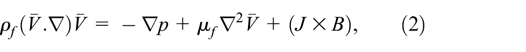
This study aims to utilize a nonlinear HSFHFM to investigate the STDTHNFF over a spinning disk. It examines the thermophysical properties of kerosene oil as a base fluid with ternary nanomaterials (Ag, $Mn Zn F e_{2} O_{4}$ , and Cu). The system of nonlinear partial differential equations is reformulated into a dimensionless form using suitable similarity transformations. The RNN-LMM is employed for backpropagation, providing an efficient and accurate computational approach for solving the problem. The accuracy and reliability of the proposed methodology are validated through EH analyses, RG metrics, time response graphs, and error analyses. The study’s original findings are significant and applicable in various domains, including predictive modeling and computational fluid dynamics. For the solution MATLAB 2023 is used for computational purposes.

Governing equation

A steady two-dimensional flow of a THNF, composed of nanomaterials ( $Ag, MnZnF e_{2} O_{4}$ , and Cu) dispersed in kerosene oil as the base fluid, is analyzed over a disk while considering the effects of asymmetrical thermal propagation and CCHF. We chose Ag, Cu, and MnZnFe₂O₄ for kerosene-based nanofluids due to their excellent thermal and functional properties. Ag provides high thermal conductivity and antimicrobial effects, while Cu enhances heat transfer efficiency. $Mn Zn F e_{2} O_{4}$ adds magnetic responsiveness and thermal stability, making the nanofluid suitable for advanced industrial applications. The spinning disk spins with an angular velocity (Ω), where (T_w) represents its uniform temperature, and ( $T_{\infty}$ ) denotes the free stream temperature. A uniform magnetic field (B₀) is applied parallel to the z-axis. Figure 1 illustrates the velocity components $(u, v, w)$ along the $(r, φ, z)$ directions. The governing equations in vector form are given in [31, 52].

\nabla . \bar{V} = 0,

(1)

ρ_{f} (\bar{V} . \nabla) \bar{V} = - \nabla p + μ_{f} \nabla^{2} \bar{V} + (J \times B),

(2)

(\bar{V} . \nabla) T = α_{f} \nabla^{2} T + τ [D_{B} (\nabla T) + \frac{D_{T}}{T_{\infty}} {(\nabla T)}^{2}] .

(3)

Figure 1.

Geometry of present investigation.

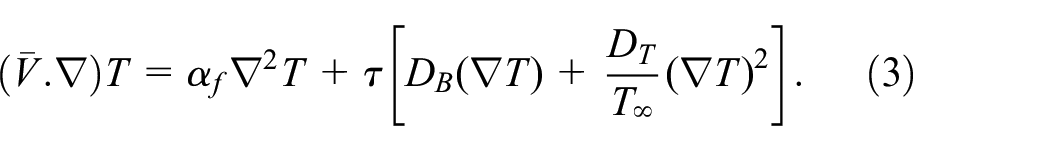
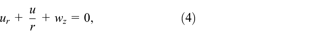
In component form [31, 52], we have:

u_{r} + \frac{u}{r} + w_{z} = 0,

(4)

\begin{matrix} ρ_{thnf} (u u_{r} - \frac{v^{2}}{r} + w u_{z}) + p_{r} = μ_{thnf} \\ (u_{rr} + \frac{1}{r} u_{r} - \frac{u}{r^{2}} + u_{zz}) - σ_{thnf} B_{0}^{2} u, \end{matrix}

(5)

\begin{matrix} ρ_{thnf} (u v_{r} - \frac{uv}{r} + w v_{z}) = μ_{thnf} (v_{rr} + \frac{1}{r} v_{r} - \frac{v}{r^{2}} + v_{zz}) \\ - σ_{thnf} B_{0}^{2} v, \end{matrix}

(6)

ρ_{thnf} (u w_{r} + w w_{z}) + p_{r} = μ_{thnf} (w_{rr} + \frac{1}{r} w_{r} + w_{zz}),

(7)

\begin{matrix} (ρ C_{P})_{thnf} (u T_{r} + w T_{z}) = K_{thnf} (T_{rr} + \frac{1}{r} T_{r} + T_{zz}) \\ - {(q_{r})}_{z} + Q (T - T_{\infty}) \\ - Γ [u^{2} T_{rr} + w^{2} T_{zz} + 2 uw T_{rz} + (u u_{r} + w u_{z}) T_{r} + (u w_{r} + w w_{z}) T_{z}], \end{matrix}

(8)

In the above equations, $u, v$ , and w represent the velocity components in the $r, φ$ , and z-directions, respectively, while T represents the temperature of the THNF. The density, viscosity, thermal conductivity, heat capacity, and electric conductivity of the THNF are represented by ρ_thnf, μ_thnf, K_thnf, $(ρ C_{P})_{thnf}$ , and σ_thnf. Furthermore, Γ denotes the thermal relaxation time coefficient, Q is the heat source coefficient, p represents the pressure, and B₀ represents the magnetic field strength.

Heat flux (q_r) is:

q_{r} = \frac{- 4 σ^{*}}{3 k^{*}} (T_{Z}^{4}) = \frac{- 16 σ^{*}}{3 k^{*}} T^{3} T_{z} .

(9)

Where $σ^{*}$ denotes the Stefan-Boltzmann constant, and k^* shows the absorption coefficient. Substituting equation (9) into equation (8), equation (8) reduces to:

\begin{matrix} (ρ C_{P})_{thnf} (u T_{r} + w T_{z}) = K_{thnf} (T_{rr} + \frac{1}{r} T_{r} + T_{zz}) \\ + \frac{16 σ^{*}}{3 k^{*}} \frac{δ}{δ z} (T^{3} T_{z}) + Q (T - T_{\infty}) \\ - Γ [u^{2} T_{rr} + w^{2} T_{zz} + 2 uw T_{rz} + (u u_{r} + w u_{z}) T_{r} + (u w_{r} + w w_{z}) T_{z}] . \end{matrix}

(10)

The BCs are as follows³¹:

{\begin{matrix} w = w_{0}, u = 0, v = Ω r, T = T_{w}, at z = 0, \\ T \to T_{\infty}, p \to p_{\infty} u \to 0, v \to 0, at z \to \infty . \end{matrix}

(11)

The suitable variables are:

{\begin{matrix} v = r Ω g, u = r Ω f^{'}, w = - \sqrt{2 Ω v_{f}} f, \\ ξ = \sqrt{\frac{2 Ω}{v_{f}}} z, p = p_{\infty} + 2 Ω μ_{f} p (ξ), θ (ξ) = \frac{T - T_{\infty}}{T_{w} - T_{\infty}} . \end{matrix}

(12)

The following are the dimensionless results obtained by applying similarity transformation to govern partial differential equations:

2 f ″' + \frac{N_{1}}{N_{4}} (2 ff ″ - {f^{'}}^{2} + g^{2}) - \frac{N_{5}}{N_{4}} {Maf}^{'} = 0,

(13)

2 g ″ + \frac{N_{1}}{N_{4}} (2 {fg}^{'} - 2 f^{'} g) - \frac{N_{5}}{N_{4}} Mag = 0,

(14)

\begin{matrix} \frac{1}{\Pr} (θ ″ + \frac{4 Nr}{3 N_{3}} \frac{d}{d ξ} {{(1 + (θ_{w} - 1) θ (ξ))}^{3} \frac{d θ (ξ)}{d ξ}}) \\ + \frac{N_{2}}{N_{3}} f θ^{'} + \frac{γ}{N_{3}} θ - \frac{N_{2}}{N_{3}} Q_{T} (f^{2} θ ″ + {ff}^{'} θ^{'}) = 0 . \end{matrix}

(15)

With:

{\begin{matrix} f = - S, f^{'} = 0, g = 1, θ = 1, at ξ = 0, \\ f^{'} \to 0, g \to 0, θ \to 0, as ξ \to \infty . \end{matrix}

(16)

The governing flow parameters are:

Parameter values	Notation	Parameter name
$Ma = \frac{α_{f} B_{0}^{2}}{Ω ρ_{f}}$	Ma	Magnetic parameter
$Nr = \frac{4 σ^{} T_{\infty}^{3}}{3 k^{} K_{f}}$	Nr	Thermal radiation parameter
$Q_{T} = 2 Γ Ω$	Q _T	Thermal relaxation parameter
$\Pr = \frac{μ_{f} {(ρ C_{P})}_{f}}{ρ_{f} K_{f}}$	Pr	Prandtl number
$S = \frac{w_{0}}{\sqrt{2 Ω v_{f}}}$	S	Suction and injection parameter
$θ_{w} = \frac{T_{w}}{T_{\infty}}$	θ _w	Temperature ratio parameter
$γ = \frac{Q}{2 Ω {(ρ C_{p})}_{f}}$	γ	Heat source-sink parameter
$N_{1} = \frac{ρ_{thnf}}{ρ_{f}}$	N ₁	Constant
$N_{2} = \frac{{(ρ C_{P})}_{thnf}}{{(ρ C_{P})}_{f}}$	N ₂	Constant
$N_{3} = \frac{K_{thnf}}{K_{f}}$	N ₃	Constant
$N_{4} = \frac{μ_{thnf}}{μ_{f}}$	N ₄	Constant
$N_{5} = \frac{σ_{thnf}}{σ_{f}}$	N ₅	Constant

The essential engineering parameters are as follows:

\begin{matrix} C_{fr} = {Re}_{z}^{\frac{1}{2}} C_{f} \\ = (\frac{{(1 - ϕ_{' 1} - ϕ_{' 2} - ϕ_{' 3})}^{- 2.5}}{(1 - ϕ_{' 1} - ϕ_{' 2} - ϕ_{' 3}) + ϕ_{' 1} (\frac{ρ_{1}}{ρ_{f}}) + ϕ_{' 2} (\frac{ρ_{2}}{ρ_{f}}) + ϕ_{' 3} (\frac{ρ_{3}}{ρ_{f}})}) f ″ (0), \end{matrix}

(17)

\begin{matrix} C_{gr} = {Re}_{z}^{\frac{1}{2}} C_{g} \\ = (\frac{{(1 - ϕ_{' 1} - ϕ_{' 2} - ϕ_{' 3})}^{- 2.5}}{(1 - ϕ_{' 1} - ϕ_{' 2} - ϕ_{' 3}) + ϕ_{' 1} (\frac{ρ_{1}}{ρ_{f}}) + ϕ_{' 2} (\frac{ρ_{2}}{ρ_{f}}) + ϕ_{' 3} (\frac{ρ_{3}}{ρ_{f}})}) g^{'} (0), \end{matrix}

(18)

N u_{r} = \frac{Nu}{\sqrt{{Re}_{z}}} = - \frac{K_{thnf}}{K_{f}} (1 + \frac{4 Nr}{3 N_{3}} {1 + (θ_{w} - 1) θ (0)}^{3}) θ^{'} (0) .

(19)

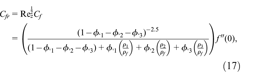
Where C_fr is the dimensionless radial skin friction, C_gr is the dimensionless tangential skin friction, and Nu_r is the reduced Nusselt number, and ${Re}_{z}$ is the Reynolds number along the axial direction.

Numerical method

Recurrent neural networks (RNN)

A prime instance of a neural network that can readily manage big datasets is the RNN, which loops backward through each unit’s historical data. The RNN makes use of the number of start function components for the respective time step. The hidden state is an internal state that exists in every one of these components. The information from the past that the unit processed previously and stored at that particular time step is represented by the hidden state. To reflect the most recent knowledge, this state information is updated frequently at every time step. In RNN, the hidden state is updated by using the recurrence relation. One time step of input is supplied at a time ‘t’. The network’s inputs and the value of the previous state are then used to calculate the current state. The computed current state, denoted as h_t will now be used as the prior state value at time t−1 for the subsequent time step. Thus, the recent state ‘h_t’ at time ‘t’ updates the preceding state ‘h_t−1’ at the time period ‘t−1’. The output is computed for all the time steps. The ultimate current state is computed when each time step is finished. The final current state is used to calculate the recurrent network’s ultimate output. The difference between the calculated and actual outputs is then used to calculate the error value. Next, the weights are updated and this error is backpropagated through the network.

Network architecture

Multi-layer neural networks have been employed in network infrastructure for learning purposes since they may be used to learn nonlinear as well as various decision-making problems. The most common type of multilayer neural network training method is error back-propagation. As shown in Figure 2, the input, hidden, and output layers make up the neural network’s structure. At the input layer, neural network inputs are collected. One neuron is taken into consideration for each input data set, and the number of neurons is chosen based on the number of input parameters. It is simpler to train a neural network and use prior knowledge for new inputs because of its hidden component. The output layer, which establishes the network’s output values, is a neural network’s third component. The feed-forward network infrastructure is taken into account at the hidden layer, and the network’s transfer function is the sigmoid function. The architecture of the RNN-LMM based on 15 neurons with a sigmoid activation function is exposed in Figure 2. The orientation information set of RNN-LMM for problems is generated using 100 input grids within the intervals [0, 1].

Figure 2.

Architecture RNN-LMM.

Learning process

Figure 3 presents the step-by-step workflow of the intended technique. The output of the RNN-LMM is generated using the Matlab toolbox for a two-layer feedforward network with back-propagation, as shown in Figure 4.

Figure 3.

Overall functional flow chart.

Figure 4.

Output of STDTHNFF with non-linear HSFHFM over a spinning disk using RNN-LMM.

Results and discussion

Performance graphs

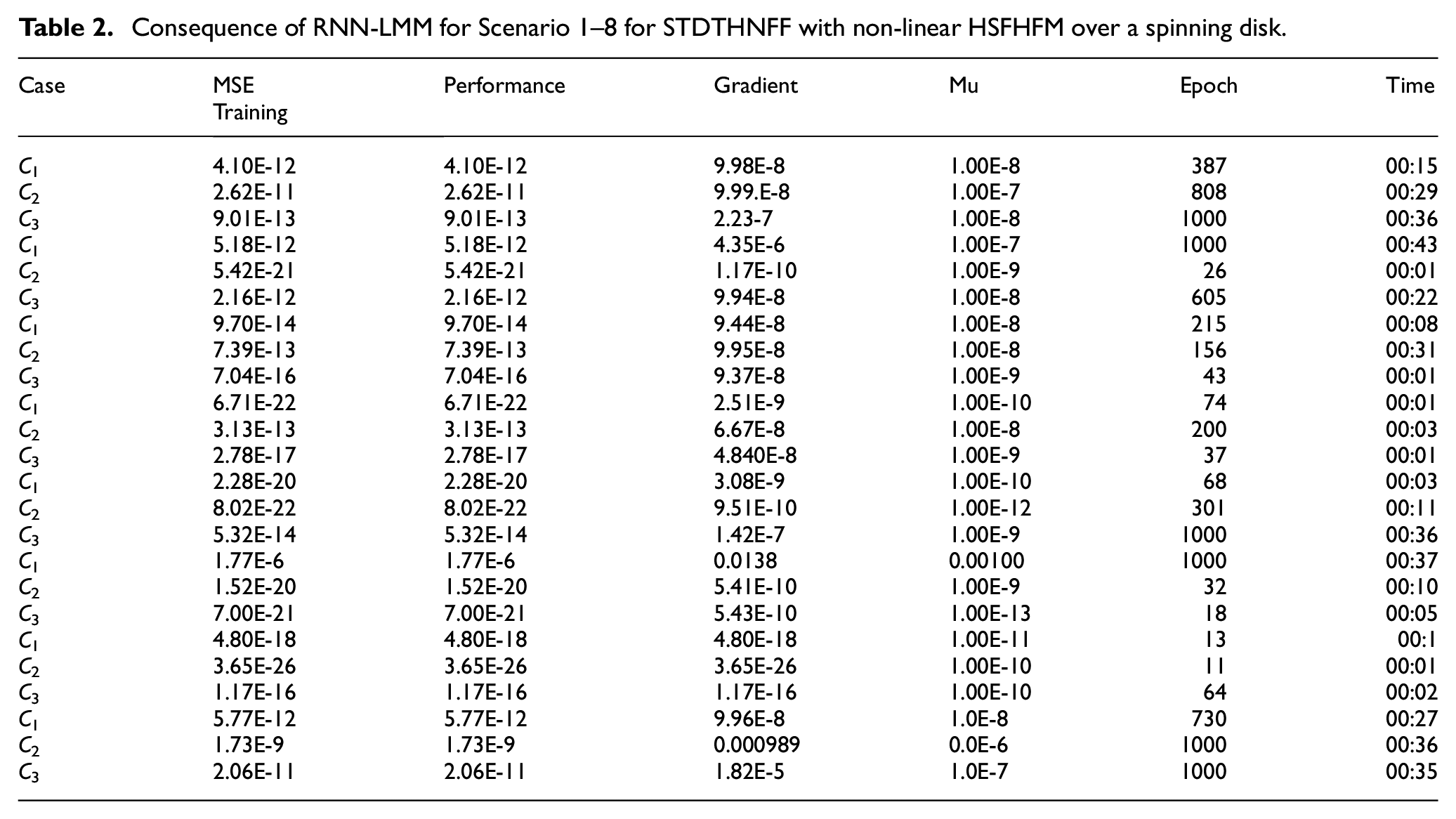
The outcome of RNN-LMM for Case 1 of all scenarios in relation to PF and states is presented in Figure 5(a) to (h) and Figure 5, respectively, while EH and time series response are shown in Figure 6(a) to (h) and Figure 6, respectively. The RG analysis is provided in Figure 7 for all scenarios of Case 1 for STDTHNFF with non-linear HSFHFM over a spinning disk. Input error cross-correlation and error auto-correlation of ANN-LMM for Case 1 of all scenarios of STDTHNFF with non-linear HSFHFM over a spinning disk are presented in Figure 8(a) to (h) and 8, respectively. In Figure 5(a) to (h), For Case 1 under all limitations, the convergence of the MSE for training procedure is shown for STDTHNFF with non-linear HSFHFM over a spinning disk. The best network performance is achieved at 4.0989 E-12 at epoch 387, 5.1767 E-12 at epoch 1000, 9.703E-14 at epoch 215, 6.7139E-22 at epoch 74, 2.2798E-20 at epoch 68, 1.7652 E-6 at the epoch 1000, 4.800 E-18 at epoch 13, and 5.5773 E-12 at epoch 730. The gradient and step size Mu of back-propagation are approximately [9.9819E-8, 4.3531E-6, 9.4418E-8, 2.5054 E-9, 3.0756E-9, 0.013807, 8.5549E-8, and 9.964 E-8] and [E-8, E-7, E-8, E-10, E-10, 0.001, E-11, and E-8] respectively, as shown in Figure 5(a1) to (h1). The results display the accuracy and convergence of the PF of RNN-LMM for each case.

Figure 5.

(a,a1 to h,h1): Predicted RNN-LMM, PF results of MSE and State transition dynamics for Case 1 of all STDTHNFF scenarios with non-linear HSFHFM over a rotating disk.

Figure 6.

(a,a1 to h,h1): EH and approximate solution with error analysis of time series response of RNN-LMM for Case 1 across all scenario of STDTHNFF with non-linear HSFHFM over a spinning disk.

Figure 7.

(a-h): RNN-LMM regression representation for Case 1 across all STDTHNFF scenarios involving non-linear HSFHFM across a rotating disk.

Figure 8.

(a,a1 to h,h1): Input error cross correlation and error auto-correlation of RNN-LMM for Case 1 of all scenario of STDTHNFF with non-linear HSFHFM over a spinning disk.

Error graphs

Figure 6(a) to (h), Figure 8 show the error visualizations and Figure 6(a1) to (h1) show time series response error. Graphs from 6(a) to (h), display the error histogram plot while Figure 6(a1) to (h1) shows the error analysis plots. Consequently, the error value and error frequency are plotted on the vertical and horizontal axes, respectively. Using the prediction of the network based on the input data, output data, and TR method, the weights are adjusted to obtain the intended results. A negative deviation will appear on the EH graph when the output value is larger than the desired value. If the bars are longer in the neighborhood of the zero-error stripe, the network is likely well-trained. The RNN-LMM generated outcomes are compared with reference numerical results for Case 1 under all conditions, and the respective results are given beside the error dynamics for input between 0 and 1 with a step size of 0.01. The highest error attain for TR are less than 59 × E-5, 35 × E-5, 59 × E-6, 59 × E-10, 60 × E-10, 25 × E-3, 18 × E-9, and 52 × E-5 for case 1 of all scenarios. The error details are further calculated with EH for each input parameter, and outcomes are given in Figure 6(a) to (h), for Case 1 of all scenarios, respectively, of flow problem. The error distribution with orientation zero line has error around −3.5 × E-7, −3.8 × E-7, 3.82 × E-8, −2.1 × E-12, 3.63 × E-13, 1.71 × E-5, −1.9 × E-11, and −3.3 × E-7 for all scenarios of flow problem. Figure 8(a) to (h) and (a₁) to (h₁), show error input-correlations and error auto-correlation, respectively. In the Figure 8(a) to (h) show the input-correlation error between the input one and error one. The error is 1.2 × E-7, 1.3 × E-7, 0.6 × E-8, 8 × E-12, 6 × E-11, 0.8 × E-4, 10 × E-11, and 1 × E-7, respectively. In the subfigures 8(a₁) to (h₁) shows the correlation one. The error is analyzed is 23 × E-21, 5.1 × E-12, 1.8 × E-6, 7 × E-22, 24 × E-21, 1.8 × E-6, 5 × E-18, and 6 × E-12, respectively.

Regression graphs

Figure 7 represents the regression display. The independent and predicted values are represented, respectively, by the regression displays’ horizontal and vertical axes. All the circles represent the data on the line, and the lines are at 45-degree angle. Therefore, the data is correct. The y-intercept, slope, and regression values are central components. The exploration throughout RG is also studies using Correlation (R) training. The R-value is frequently close to 1, which acknowledges the RNN-LMM implementation for the model problem.

Velocity and temperature profiles

This section analyzes the behavior of the velocity components $f^{'} (η)$ and $g (η)$ along with the temperature $θ (η)$ , under the influence of various emerging physical parameters. Figures 9(a), 10(a), and 11(a) show the effect of the magnetic parameter (Ma), suction and injection parameter S, and nanoparticle volume fraction ( $ϕ_{3}$ ) on the velocity profile. Figure 9(a) illustrates the effect of the Ma on the velocity distribution profile ( $f^{'} (η)$ ). As the magnetic parameter increases, the velocity profile declines. Physically, the negative Lorentz force leads to a reduction in fluid flow. The magnetic field acts against the motion of the fluid, generating resistance. Consequently, the presence of the Lorentz force hinders the flow, leading to a decline in flow velocity and a thinning of the momentum boundary layer. Figure 10(a) depicts the influence of the suction and injection parameter (S) on the velocity distribution profile $f^{'} (η)$ . As the suction and injection parameter S increases, the velocity distribution ( $f^{'} (η)$ ) also rises. Physically, an increase in the S influences the fluid flow by modifying momentum transfer. When S increases due to injection (S > 0), additional fluid is introduced into the system, enhancing the velocity and thickening the boundary layer. This leads to increased energy within the flow, reducing resistance and promoting faster movement. Conversely, suction (S < 0) extracts fluid, lowering velocity and thinning the boundary layer by reducing available momentum. Figure 11(a) examines the effect of the nanoparticle volume fraction (ϕ₃) on the velocity distribution profile $f^{'} (η)$ . The velocity profile $f^{'} (η)$ increases with higher nanoparticle volume fractions. Physically, incorporating tri-hybrid nanomaterials into the base fluid enhances its overall viscosity, leading to a reduction in fluid motion. Figures 9(c), 10(c), and 11(c) illustrate the effects of Ma, S, and $ϕ_{3}$ on the velocity curve ( $g (η)$ ). Figure 9(c) investigates the effect of the Ma on the motion pattern. An increase in Ma reduces the movement gradient ( $g (η)$ ), a characteristic commonly observed in MHD flows for both classical and non-traditional fluids under various physical conditions. Figure 10(c) shows the result of S on the velocity profile $g (η)$ . As the parameter S rises in the basic fluid, the velocity profile $g (η)$ decreases. Figure 11(c) illustrates the effect of the particulate volume fraction ( $ϕ_{3}$ ) on the trajectory curve ( $g (η)$ ). The velocity curve increases as the particulate volume ratios ( $ϕ_{3}$ ) rise. Figure 9(e), 10(e), and 11(e) illustrate the influences of Ma, S, and $ϕ_{3}$ on the temperature profile $θ (η)$ . The impact of the magnetic parameter (Ma) on the thermal profile ( $θ (η)$ ) is shown in Figure 9(e). The temperature profile $θ (η)$ flow is maximized by applying the concept of larger Ma values. As the magnetic parameter increases, the Lorentz force acts as a resistive force, slowing down the fluid motion. This reduction in velocity weakens convective heat transfer, causing heat to accumulate within the fluid. As a result, thermal diffusion dominates, leading to an upsurge in the temperature profile. Thus, higher (Ma) values enhance heat retention and thermal distribution in the fluid. Figure 10(e) analyzed the effects of S on the thermal profile $θ (η)$ . The thermal profile $θ (η)$ decreases as the magnitude of S increases. The fluid flow in the channel is controlled by a suction/injection method, and an Arrhenius locomotive heat-releasing chemical reaction is investigated. The numerical results about the various factors entangled in the problem are presented both mathematically and graphically. Figure 11(e) illustrates the effect of the nanoparticle volume fraction ( $ϕ_{3}$ ) on the $θ (η)$ . Physically, as the volume fraction ( $ϕ_{3}$ ) increases, the thermal profile $θ (η)$ becomes more pronounced. As the nanoparticle volume fraction increases, thermal conductivity improves, enhancing heat transfer. This leads to greater heat absorption and retention, raising the temperature profile. Additionally, nanoparticles reduce thermal resistance, allowing heat to spread more efficiently. As a result, the temperature distribution profile becomes more pronounced. Figure 12(a) presents the influence of the temperature ratio parameter (θ_w) on the temperature distribution curve ( $θ (η)$ ). An increase in θ_w enhances, the temperature distribution, making the profile more prominent. Figure 13(a) highlights the significance of the thermal relaxation parameter (Q_T) on the thermal field. An increase in Q_T results in a decrease in Thermal distribution profile $θ (η)$ . Physically, the thermal relaxation parameter (Q_T) represents the time delay in heat conduction, as described by the CCHFM. When Q_T increases, the fluid takes longer to respond to temperature changes, reducing heat diffusion. This weakens thermal conductivity, leading to a decline in the thermal distribution profile. As a result, heat spreads more slowly throughout the fluid, lowering overall temperature gradients. Plotting is performed in Figure 14(a) to examine how the thermal radiation parameter Nr affects the $θ (η)$ . The higher greatness of the Nr increased $θ (η)$ . The heating radiation parameter determines the degree to which heat conductance movement affects the dispersion of heat sun light. Improving the light component increases the boundary layer’s elevation, cross-flow rate, and velocity. Figure 15(a) examines the influence of the Prandtl number (Pr) on the $θ (η)$ . Higher values of Pr lead to a reduction in the thermal distribution profile ( $θ (η)$ ). As a dimensionless parameter, the Prandtl number represents a fluid’s inherent characteristics. Fluids with lower Pr values have higher thermal conductivity, allowing efficient heat transfer and making them ideal for heat-conducting applications. Figure 16(a) show the outcome of the heat source parameter γ in temperature distribution profile $θ (η)$ . The values of the γ increases then the results temperature distribution profile $θ (η)$ increases. Physically, this happens because the additional heat input enhances molecular agitation, increasing the internal energy of the fluid and raising its temperature.

Figure 9.

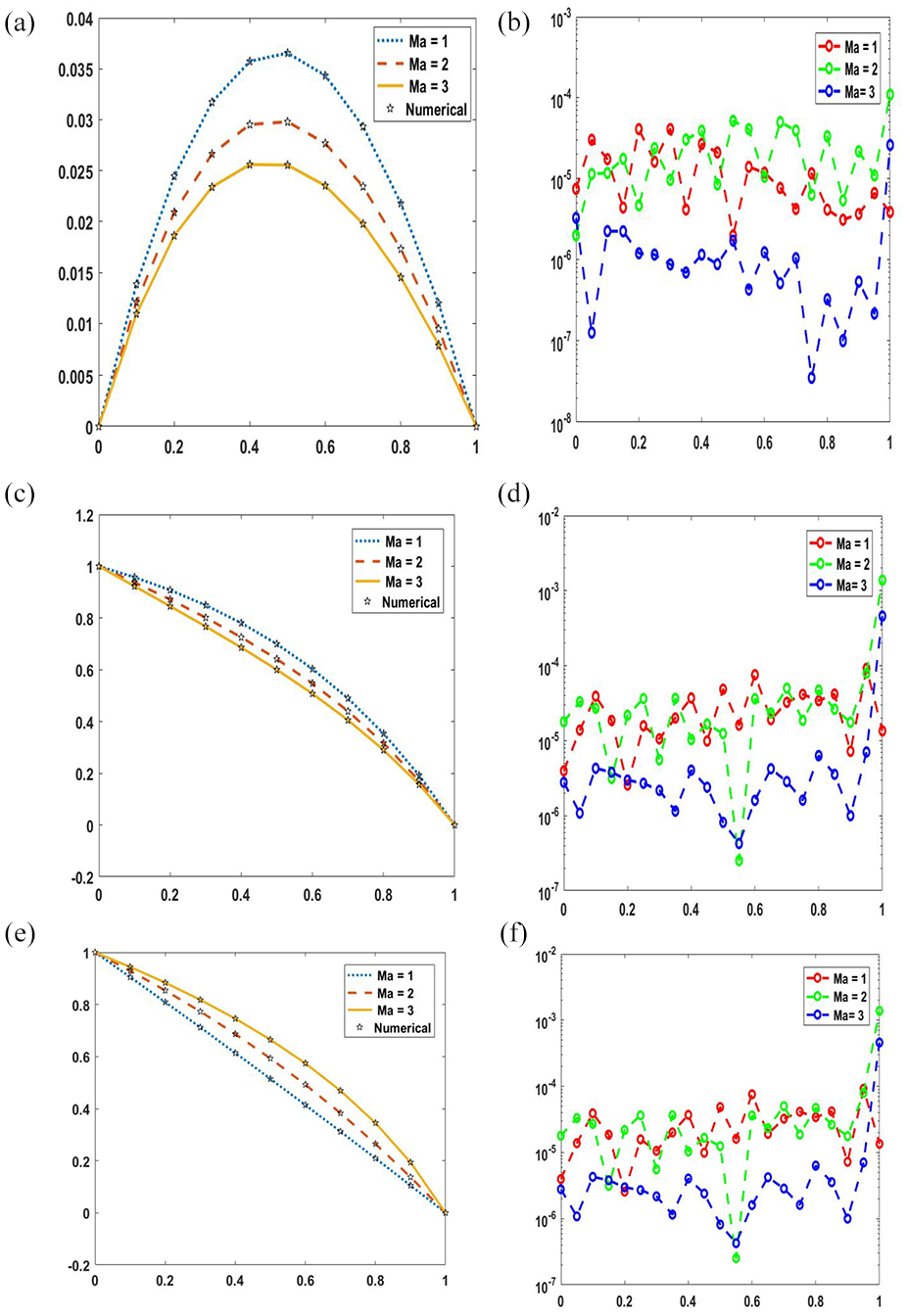
Assessment of proposed RNN-LMM for Case 1 of all scenario of STDTHNFF with non-linear HSFHFM over a spinning disk: (a) variation of the Ma in f′, (b) error display of the Ma in f′, (c) variation of the Ma in g, (d) error display of the Ma in g, (e) variation of the Ma in $θ (η)$ , and (f) error display of the Ma in $θ (η)$ .

Figure 10.

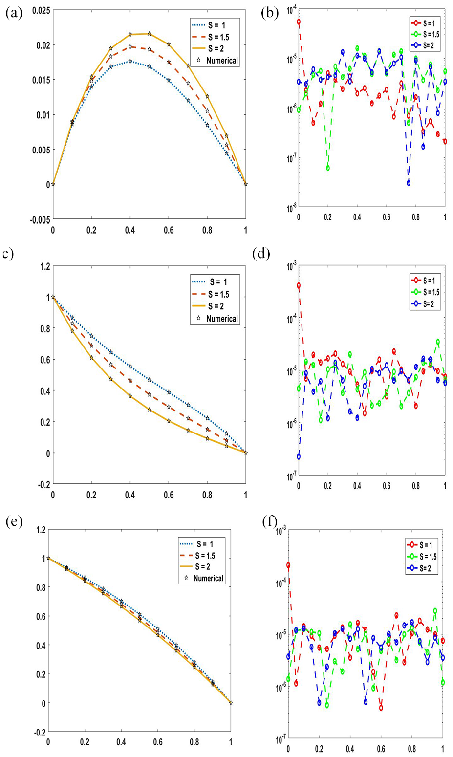
Assessment of proposed RNN-LMM for Case 1 of all scenario of STDTHNFF with non-linear HSFHFM over a spinning disk: (a) variation of the S in f′, (b) error display of the S inf′, (c) variation of the S in g, (d) error display of the S in g, (e) variation of the S in θ, and (f) error display of the S in θ.

Figure 11.

Assessment of proposed RNN-LMM for Case 1 of all scenario of STDTHNFF with non-linear HSFHFM over a spinning disk: (a) variation of the ϕ₃ in f′, (b) error display of the ϕ₃ in f′, (c) variation of the ϕ₃ in g, (d) error display of the ϕ₃ in g, (e) deviation of the ϕ₃ in θ, and (f) error display of the ϕ₃ in θ.

Figure 12.

Assessment of proposed RNN-LMM for Case 1 of all scenario of STDTHNFF with non-linear HSFHFM over a spinning disk: (a) deviation of the θ_w in θ and (b) error display of the θ_w in θ.

Figure 13.

Assessment of proposed RNN-LMM for Case 1 of all scenario of STDTHNFF with non-linear HSFHFM over a spinning disk: (a) deviation of the Q_T in θ and (b) error display of the Q_T in θ.

Figure 14.

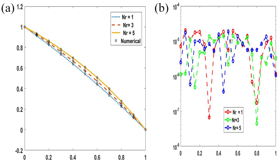
Assessment of proposed RNN-LMM for Case 1 of all scenario of STDTHNFF with non-linear HSFHFM over a spinning disk: (a) deviation of the Nr in θ and (b) error display of the Nr in θ.

Figure 15.

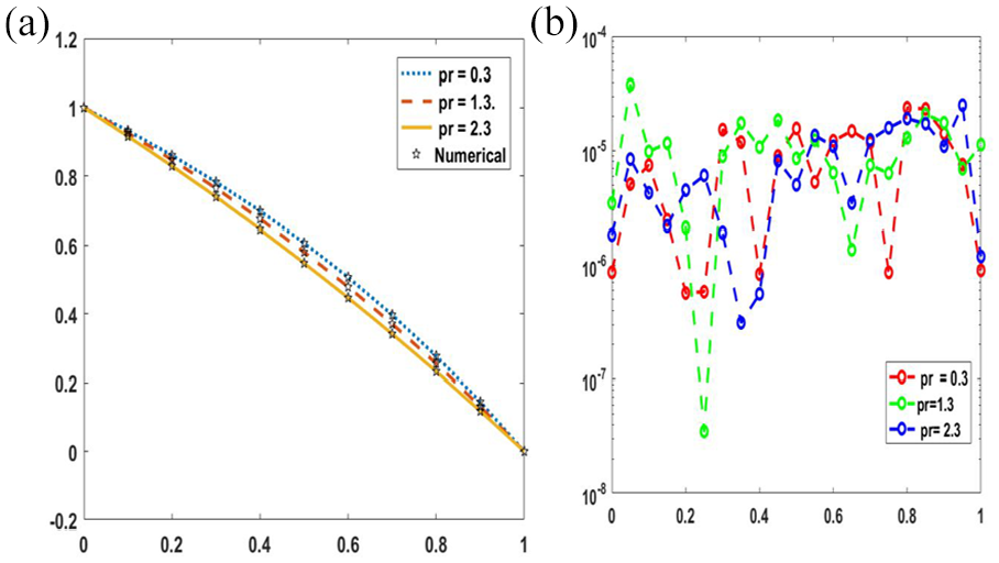
Assessment of proposed RNN-LMM for Case 1 of all scenario of STDTHNFF with non-linear HSFHFM over a spinning disk: (a) deviation of the Pr in θ and (b) error display of the Pr in θ.

Figure 16.

Assessment of proposed RNN-LMM for Case 1 of all scenario of STDTHNFF with non-linear HSFHFM over a spinning disk: (a) deviation of the γ in θ and (b) error display of the γ in θ.

Absolute error (AE) in velocity and temperature profile

The results of RNN-LMM are derived for the velocity and temperature profiles $f^{'} (η), g (η)$ , and $θ (η)$ for all parameter. Outcomes of these profiles are illustration in Figures 9 to 16 for all parameters, respectively using RNN-LMM for Case 1 of all scenarios of STDTHNFF with non-linear HSFHFM over a spinning disk. The results are displayed in subfigures 9(b), 9(d), 10(b), 10(d), 10(f), 11(b), 11(d), 11(f), 12(b), 13(b), 14(b), 15(b), and 16(b) for Case 1 studies of all parameters, respectively. Absolute errors from the aligned answer are abridged to indicate the correctness level. AE are about $10^{- 6} to 10^{- 4}$ , $10^{- 6} to 10^{- 4}$ , $10^{- 8} to 10^{- 5}$ , $10^{- 6} to 10^{- 4}$ , $10^{- 7} to 10^{- 3}$ , $10^{- 7} to 10^{- 3}$ , $10^{- 7} to 10^{- 4}$ , $10^{- 7} to 10^{- 5}$ , $10^{- 8} to 10^{- 5}$ , $10^{- 6} to 10^{- 3}$ , $10^{- 6} to 10^{- 4}$ , $10^{- 7} to 10^{- 5}$ , $10^{- 7} to 10^{- 3}$ , $10^{- 7} to 10^{- 4}$ , $10^{- 6} t o 10^{- 5}$ , $10^{- 6} to 10^{- 3}$ , $10^{- 6} to 10^{- 4}$ , $10^{- 7} to 10^{- 4}$ , $10^{- 5} to 10^{- 3}$ , $10^{- 7} to 10^{- 4}$ , $10^{- 7} to 10^{- 3}$ , $10^{- 6} to 10^{- 5}$ , $10^{- 6} to 10^{- 4}$ , $10^{- 6} to 10^{- 3}$ , $10^{- 4} to 10^{- 2}$ , $10^{- 6} to 10^{- 3}$ , $10^{- 4} to 10^{- 2}$ , $10^{- 3} to 10^{- 1}$ , $10^{- 6} to 10^{- 4}$ , $10^{- 7} to 10^{- 3}$ , $10^{- 7} to 10^{- 5}$ , $10^{- 8} to 10^{- 5}$ , $10^{- 7} to 10^{- 5}$ , $10^{- 6} to 10^{- 4}$ , $10^{- 8} to 10^{- 4}$ , $10^{- 7} to 10^{- 5}$ , $10^{- 8} to 10^{- 4}$ , $10^{- 7} to 10^{- 5}$ , and $10^{- 7} to 10^{- 5}$ for all scenarios correspondingly.

Skin friction and Nusselt number

Figure 17 demonstrates how various parameters affect skin friction and the Nusselt number. Figure 17(a) illustrates the impact of the nanoparticle volume fraction ( $ϕ_{1} = ϕ_{2} = ϕ_{3}$ ) and the magnetic parameter (Ma) on skin friction ( $C_{f} {Re}_{z}^{0.5}$ ). It is noted that as ( $ϕ_{1} = ϕ_{2} = ϕ_{3}$ ) increases, skin friction ( $C_{f} {Re}_{z}^{0.5}$ ) also rises. Furthermore, $C_{f} {Re}_{z}^{0.5}$ demonstrates higher estimated values. Figure 17(b) illustrates the effect of nanoparticle volume fraction ( $Φ_{1} = Φ_{2} = Φ_{3}$ ) and the thermal radiation (Nr) on skin fraction ( $C_{f} {Re}_{z}^{0.5}$ ). With an increase in nanoparticle volume fraction, the skin friction coefficient increases as a result of enhanced viscosity and greater flow resistance. Enhanced thermal radiation further modifies the temperature and velocity profiles, leading to an additional increase in skin friction. Figure 17(c) depicts the fluctuations in Nusselt number ( $Nu {Re}_{z}^{- 0.5}$ ) due to the influence of the nanoparticle volume fraction ( $ϕ_{1} = ϕ_{2} = ϕ_{3}$ ) and the magnetic parameter (Ma). It is evident that the local Nusselt number ( $Nu {Re}_{z}^{- 0.5}$ ), increases as the volume fraction of nanoparticles ( $ϕ_{1} = ϕ_{2} = ϕ_{3}$ ) increases. Figure 17(d) shows the fluctuation in $Nu {Re}_{z}^{- 0.5}$ for different values of Q_T along the direction of Nr. Additionally, the analysis of the figure reveals that the Nusselt number reductions with increasing values of the associated parameters Nr and Q_T.

Figure 17.

Representation of skin friction and the Nusselt number: (a) fluctuation in skin friction due to the effects of ϕ₃ and Ma, (b) fluctuation in skin friction due to the effects of ϕ₃ and Nr, (c) fluctuation in the Nusselt number caused by ϕ₃ and Ma, and (d) fluctuation in the Nusselt number caused by Q_T and Nr.

Tables analysis

The table of RNN-LMM is executed for one to eight scenarios by deviation of $Ma, S, ϕ_{3}, θ_{w}, Q_{T,} Nr, \Pr$ , and γ. In every case, there is one variable scenario and the other scenarios are fixed and listed in Table 1. Table 2 provide the outcomes of the RNN-LMM approach used to solve each case in each of the 1–8 flow problem scenarios. The PF of RNN-LMM is around $10^{- 12} to 10^{- 13}$ , $10^{- 12} to 10^{- 12}$ , $10^{- 14} to 10^{- 16}$ , $10^{- 22} to 10^{- 17}$ , $10^{- 20} to 10^{- 14}$ , $10^{- 6} to 10^{- 21}$ , $10^{- 18} to 10^{- 16}$ , and $10^{- 12} to 10^{- 11}$ for the respective 1–8 scenario cases of the flow problem. These outcomes show the reliable PF of RNN-LMM for solving flow the problem. Table 3 provides the thermophysical properties of the base fluid with embedded nanoparticles, while Table 4 highlights the thermophysical properties of THNF, HNF, and nanofluids. Table 5 presents the assessment of the tiny particle portion of volume ( $ϕ_{1} = ϕ_{2} = ϕ_{3}$ ) and S values viaC_f. Table 6 shows the assessment of $ϕ_{1} = ϕ_{2} = ϕ_{3}$ , S, and Pr values Nu.

Table 1.

Explanation of every situation in addition to every case for STDTHNFF employing a spinning disk, a non-linear HSFHFM.

Scenarios	Case	Physical volumes
		Ma	S	ϕ ₃	θ _w	Q _T	Nr	Pr	γ
1	C ₁	1	0.5	0.1	1.3	1.5	0.6	0.5	0.3
	C ₂	2	0.5	0.1	1.3	1.5	0.6	0.5	0.3
	C ₃	3	0.5	0.1	1.3	1.5	0.6	0.5	0.3
2	C ₁	1.2	1	0.1	1.3	1.5	0.6	0.5	0.3
	C ₂	1.2	1.5	0.1	1.3	1.5	0.6	0.5	0.3
	C ₃	1.2	2	0.1	1.3	1.5	0.6	0.5	0.3
3	C ₁	1.2	0.5	0.01	1.3	1.5	0.6	0.5	0.3
	C ₂	1.2	0.5	0.05	1.3	1.5	0.6	0.5	0.3
	C ₃	1.2	0.5	0.09	1.3	1.5	0.6	0.5	0.3
4	C ₁	1.2	0.5	0.1	1.3	1.5	0.6	0.5	0.3
	C ₂	1.2	0.5	0.1	3.6	1.5	0.6	0.5	0.3
	C ₃	1.2	0.5	0.1	5.6	1.5	0.6	0.5	0.3
5	C ₁	1.2	0.5	0.1	1.3	1.1	0.6	0.5	0.3
	C ₂	1.2	0.5	0.1	1.3	2.2	0.6	0.5	0.3
	C ₃	1.2	0.5	0.1	1.3	3.3	0.6	0.5	0.3
6	C ₁	1.2	0.5	0.1	1.3	1.5	1	0.5	0.3
	C ₂	1.2	0.5	0.1	1.3	1.5	3	0.5	0.3
	C ₃	1.2	0.5	0.1	1.3	1.5	5	0.5	0.3
7	C ₁	1.2	0.5	0.1	1.3	1.5	0.6	0.3	0.3
	C ₂	1.2	0.5	0.1	1.3	1.5	0.6	1.3	0.3
	C ₃	1.2	0.5	0.1	1.3	1.5	0.6	2.3	0.3
8	C ₁	1.2	0.5	0.1	0.3	1.5	0.6	2.3	1
	C ₂	1.2	0.5	0.1	0.3	1.5	0.6	2.3	2
	C ₃	1.2	0.5	0.1	0.3	1.5	0.6	2.3	3

Table 2.

Consequence of RNN-LMM for Scenario 1–8 for STDTHNFF with non-linear HSFHFM over a spinning disk.

Case	MSE	Performance	Gradient	Mu	Epoch	Time
Case	Training	Performance	Gradient	Mu	Epoch	Time
C ₁	4.10E-12	4.10E-12	9.98E-8	1.00E-8	387	00:15
C ₂	2.62E-11	2.62E-11	9.99.E-8	1.00E-7	808	00:29
C ₃	9.01E-13	9.01E-13	2.23-7	1.00E-8	1000	00:36
C ₁	5.18E-12	5.18E-12	4.35E-6	1.00E-7	1000	00:43
C ₂	5.42E-21	5.42E-21	1.17E-10	1.00E-9	26	00:01
C ₃	2.16E-12	2.16E-12	9.94E-8	1.00E-8	605	00:22
C ₁	9.70E-14	9.70E-14	9.44E-8	1.00E-8	215	00:08
C ₂	7.39E-13	7.39E-13	9.95E-8	1.00E-8	156	00:31
C ₃	7.04E-16	7.04E-16	9.37E-8	1.00E-9	43	00:01
C ₁	6.71E-22	6.71E-22	2.51E-9	1.00E-10	74	00:01
C ₂	3.13E-13	3.13E-13	6.67E-8	1.00E-8	200	00:03
C ₃	2.78E-17	2.78E-17	4.840E-8	1.00E-9	37	00:01
C ₁	2.28E-20	2.28E-20	3.08E-9	1.00E-10	68	00:03
C ₂	8.02E-22	8.02E-22	9.51E-10	1.00E-12	301	00:11
C ₃	5.32E-14	5.32E-14	1.42E-7	1.00E-9	1000	00:36
C ₁	1.77E-6	1.77E-6	0.0138	0.00100	1000	00:37
C ₂	1.52E-20	1.52E-20	5.41E-10	1.00E-9	32	00:10
C ₃	7.00E-21	7.00E-21	5.43E-10	1.00E-13	18	00:05
C ₁	4.80E-18	4.80E-18	4.80E-18	1.00E-11	13	00:1
C ₂	3.65E-26	3.65E-26	3.65E-26	1.00E-10	11	00:01
C ₃	1.17E-16	1.17E-16	1.17E-16	1.00E-10	64	00:02
C ₁	5.77E-12	5.77E-12	9.96E-8	1.0E-8	730	00:27
C ₂	1.73E-9	1.73E-9	0.000989	0.0E-6	1000	00:36
C ₃	2.06E-11	2.06E-11	1.82E-5	1.0E-7	1000	00:35

Table 3.

Thermophysical properties of base fluid-containing nanoparticles.⁴⁹

Properties	Thermal conductivity K(W/mK)	Heat capacity $C_{p} (J / kJK)$	Density $ρ (kg / m^{3})$	Prandtl number Pr
Silver (Ag)	429	235	10,500	–
Copper (Cu)	401	385	8933	–
Manganese zinc ferrite $Mn Zn F e_{2} O_{4}$	3.9	1050	4700	–
Kerosene oil	0.15	2090	783	21

Table 4.

Thermophysical characteristics of nanofluid, HNF, and THNF.

Properties	Nanofluid
Density	$ρ_{nf} = ρ_{f} (1 - ϕ_{1}) + ϕ_{1} (ρ_{s 1})$
Viscosity	$μ_{nf} = \frac{μ_{f}}{{(1 - ϕ_{1})}^{2.5}}$
Heat capacitance	$(ρ C_{p})_{nf} = (ρ C_{p})_{f} (1 - ϕ_{1}) + ϕ_{1} (ρ C_{p})_{s 1}$
Thermal conductivity	$\frac{K_{nf}}{K_{f}} = \frac{K_{s 1} + 2 K_{f} - 2 (K_{f} - K_{s 1}) ϕ_{1}}{K_{s 1} + 2 K_{f} - (K_{f} - K_{s 1}) ϕ_{1}}$
Properties	HNF
Density	$ρ_{hnf} = (1 - ϕ_{2}) (ρ_{f} (1 - ϕ_{1}) + ϕ_{1} (ρ_{s 1})) + ϕ_{2} ρ_{s 2}$
Viscosity	$μ_{hnf} = \frac{μ_{f}}{{(1 - ϕ_{1})}^{2.5} {(1 - ϕ_{2})}^{2.5}}$
Heat capacitance	$(ρ C_{p})_{hnf} = (1 - ϕ_{2}) ({(ρ C_{p})}_{f} (1 - ϕ_{1}) + ϕ_{1} {(ρ C_{p})}_{s 1}) + ϕ_{2} (ρ C_{P})_{s 2}$
Thermal conductivity	$\frac{K_{hnf}}{K_{nf}} = \frac{K_{s 2} + 2 K_{nf} - 2 (K_{nf} - K_{s 2}) ϕ_{2}}{K_{s 2} + 2 K_{nf} + (K_{nf} - K_{s 2}) ϕ_{2}}$
Properties	THNF
Density	$ρ_{thnf} = (1 - ϕ_{3}) ((1 - ϕ_{2}) (ρ_{f} (1 - ϕ_{1}) + ϕ_{1} (ρ_{s 1})) + ϕ_{2} ρ_{s 2}) + ϕ_{3} ρ_{s 3}$
Viscosity	$μ_{thnf} = \frac{μ_{f}}{{(1 - ϕ_{1})}^{2.5} {(1 - ϕ_{2})}^{2.5} {(1 - ϕ_{3})}^{2.5}}$
Heat capacitance	$(ρ C_{p})_{thnf} = (1 - ϕ_{3}) [(1 - ϕ_{2}) ({(ρ C_{p})}_{f} (1 - ϕ_{1}) + ϕ_{1} {(ρ C_{p})}_{s 1}) + ϕ_{2} {(ρ C_{P})}_{s 2}] + ϕ_{3} (ρ C_{P})_{s 3}$
Thermal conductivity	$\frac{K_{thnf}}{K_{hnf}} = \frac{K_{s 3} + 2 K_{hnf} - 2 (K_{hnf} - K_{s 3}) ϕ_{3}}{K_{s 3} + 2 K_{hnf} + (K_{hnf} - K_{s 3}) ϕ_{3}}$

Table 5.

Comparison of ( $ϕ_{1} = ϕ_{2} = ϕ_{3}$ ), S values via C_f.

$ϕ_{1} = ϕ_{2} = ϕ_{3}$	S	Acharya et al.⁵¹	Alqawasmi et al.⁵²	Current results
0.00	1	0.389642	0.389643	0.389645
	−1	0.489511	0.489512	0.489513
	2	0.242421	0.242422	0.242424
	0	0.510205	0.510206	0.510208
	−1	0.398936	0.398937	0.398938
	1	0.389618	0.389619	0.389620
	0	0.510141	0.510142	0.510144
	−1	0.488931	0.488932	0.488933
0.1	1	0.603121	0.603122	0.603124
	0	0.550277	0.550278	0.550279
	−1	0.516733	0.516733	0.516734

Table 6.

Comparison of ( $ϕ_{1} = ϕ_{2} = ϕ_{3}$ ), S, and Pr values via Nu.

$ϕ_{1} = ϕ_{2} = ϕ_{3}$	Pr	S	Acharya et al.⁵¹	Alqawasmi et al.⁵²	Current results
0.00	0.64	1	0.720242	0.720243	0.720245
		−1	0.090675	0.090676	0.090678
	0.71	2	1.437812	1.437814	1.437815
		0	0.325969	0.325970	0.325971
		−1	0.011404	0.011406	0.011407
	6.2	1	6.272213	6.272215	6.272216
		0	0.933725	0.933727	0.933729
		−1	0.000211	0.000213	0.000214
0.1	6.2	1	4.657438	4.657439	4.657441
		0	0.821517	0.821524	0.821525
		−1	0.001638	0.001639	0.001640

Conclusions

We examined the effects of STDTHNFF with a non-linear heat source-sink and Fourier heat flux model over a rotating disk. The important consequences are as follows:

When the Ma and ϕ₃ values rise, the $f^{'} (η)$ decreases, and when the value of the S grows, the $f^{'} (η)$ increases.

As the Ma value rises, the heat distribution profile increases, and the velocity profile decreases with increasing magnetic field values.

The temperature profile increases as the values of the ϕ₃ increase.

The thermal profile declines with increasing Pr values and rises with higher amplitudes of the thermal radiation parameter and the heat source-sink parameter.

For the temperature ratio parameter, the temperature increase, and for the higher thermal relaxation parameter approximations, the temperature is decreases.

The values of the γ increases then the results temperature distribution profile $θ (η)$ increases.

RNN-LMM does not require an initial guess or linearization techniques.

Due to its capability to minimize absolute error and enhance accuracy, RNN-LMM outperforms other approaches.

RNN-LMM is widely used for regression and data fitting problems, demonstrating strong agreement with experimental or numerical data.

Practical applications

The results of this study could be applied in several engineering and industrial sectors, including:

Heat transfer enhancement in industrial systems: The study investigates THNF, which could significantly improve heat transfer in various industrial applications such as cooling systems, heat exchangers, and thermal management devices.

Nanofluid-based cooling systems: The use of manganese zinc ferrite, copper, and silver nanocomposites could lead to advancements in nanofluid-based cooling systems, which are used in electronics, automotive, and renewable energy systems to enhance the performance of heat exchangers and coolants.

Energy and environmental applications: The findings may also be applied in renewable energy systems (e.g. solar thermal systems) and environmental technologies (e.g. water purification), where efficient heat management and antimicrobial properties are essential.

Medical applications: The antibacterial properties of silver nanoparticles could also have implications in medical applications, such as wound healing, sterilization, and drug delivery systems, making them a key material in biomedical research.

Limitations and future scope

The study is limited to a 2D nonlinear Fourier heat flux model. The model can be extended to 3D geometries to gain a more comprehensive understanding of the behavior of ternary hybrid nanofluids in complex, real-world systems.

The model assumes steady-state conditions. Future work could focus on extending the model to transient conditions, where both fluid flow and temperature vary with time, better reflecting real-world operational scenarios.

The current model was developed based on specific boundary conditions (a spinning disk), which may not fully capture diverse practical scenarios. In the future, the study could be extended by generalizing the boundary conditions across various applications to enhance its applicability to real-world problems.

Experimental validation of the ARNN-LMM framework is a key area for future research to enhance the reliability and practical applicability of the proposed intelligent computing approach.

Footnotes

Appendix

Notation

(u, v, w)	Velocity components $(m / s)$	ρ _nf	Density of nanofluid $(kg / m^{3})$
$(r, ϕ, z)$	Coordinates system	ρ _nf	Viscosity of nanofluid $(kg / m s)$
$T_{\infty}$	Uniform temperature of disk (K)	$(ρ C_{P})_{nf}$	Heat capacity of nanofluid $(J / m^{3} K)$
T _w	Temperature free stream (K)	K _nf	Thermal conductivity of nanofluid $(W / mK)$
Ω	Angular velocity $(m / s)$	ρ _hnf	Density of HNF $(kg / m^{3})$
B ₀	Magnetic field $(Ω^{- 1 / 2} m^{- 1} s^{- 1 / 2} k g^{1 / 2})$	ρ _hnf	Viscosity of HNF $(kg / m s)$
C _f	Skin friction	$(ρ C_{P})_{hnf}$	Heat capacity of HNF $(J / m^{3} K)$
$Re$	Reynolds number	K _hnf	Thermal conductivity of HNF $(W / mK)$
Nu	Nusselt number	ρ _thnf	Density of THNF $(kg / m^{3})$
MSE	Mean square error	ρ _thnf	Viscosity of THNF $(kg / m s)$
RG	Regression	$(ρ C_{P})_{thnf}$	Heat capacity of THNF $(J / m^{3} K)$
TR	Training	K _thnf	Thermal conductivity of THNF $(W / mK)$
FT	Fitting	$ϕ_{1} = ϕ_{2} = ϕ_{3}$	Nanoparticle volume fraction
PF	Performance	Ag	Silver
EH	Error histograms	Cu	Copper
AI	Artificial Intelligence	$Mn Zn F e_{2} O_{4}$	Manganese zinc ferrite
ANN	Artificial neural networks	q _r	Radiative heat flux $(kg / s^{3})$
RNN	Recurrent neural networks	$σ^{*}$	Stephan-Boltzmann constant $(W / m^{2} K^{4})$
RNN-LMM	Recurrent neural networks with Levenberg-Marquardt method	k ^*	Mean absorption coefficient $(m^{- 1})$
NLPDEs	Nonlinear partial differential equations	σ _thnf	Electric conductivity (Sm⁻¹)
CCHF	Cattaneo-Christov heat flux	C _g	Tangential skin friction
C _f	Radial Skin friction	Nu	Nusselt number
CCHFM	Cattaneo-Christov heat flux model	$Re$	Reynolds number

Handling Editor: C.S.K. Raju

ORCID iDs

Hakeem Ullah

Seham M. Al-Mekhlafi

Funding

The author(s) received no financial support for the research, authorship, and/or publication of this article.

Declaration of conflicting interests

The author(s) declared no potential conflicts of interest with respect to the research, authorship, and/or publication of this article.

References

Choi

Eastman

. Enhancing thermal conductivity of fluids with nanoparticles. Report no. ANL/MSD/CP-84938; CONF-951135-29, Argonne National Lab. (ANL), Argonne, IL, USA, 1995.

Rasool

Shafiq

Wang

, et al. Numerical treatment of MHD Al₂O₃–Cu/engine oil-based nanofluid flow in a Darcy–Forchheimer medium: application of radiative heat and mass transfer laws. Int J Mod Phys B 2024; 38(9): 2450129.

Faizan

Ali

, et al. Modelling and analysis of heat transfer in MHD stagnation point flow of Maxwell nanofluid over a porous rotating disk. Alex Eng J 2024; 91: 237–248.

Mahmood

Rafique

Khan

, et al. Investigation of entropy generation in the existence of heat generation and nanoparticle clustering on porous Riga plate during nanofluid flow. Mater Today Commun 2024; 38: 108165.

Hameed

Al-Srayyih

Al-Amir

, et al. Magnetic field effect on mixed convection flow inside an oval-shaped annulus enclosure filled by a non-Newtonian nanofluid. Int J Thermofluids 2024; 21: 100571.

Yasmin

Giwa

Noor

, et al. Reproduction of nanofluid synthesis, thermal properties and experiments in engineering: a research paradigm shift. Energies 2023; 16(3): 1145.

Ajeeb

da Silva

RRT

Murshed

SS.

Experimental investigation of heat transfer performance of Al₂O₃ nanofluids in a compact plate heat exchanger. Appl Therm Eng 2023; 218: 119321.

Shamshuddin

Saeed

Asogwa

, et al. A semi-analytical approach to investigate the entropy generation in a tangent hyperbolic magnetized hybrid nanofluid flow upon a stretchable rotating disk. J Magn Magn Mater 2023; 574: 170664.

Abbas

Khan

Hashmi

, et al. Numerically analysis of Marangoni convective flow of hybrid nanofluid over an infinite disk with thermophoresis particle deposition. Sci Rep 2023; 13(1): 5036.

10.

Abas

Ullah

Fiza

, et al. Second order slip micropolar MHD hybrid nanofluid flow over a stretching surface with uniform heat source and activation energy: numerical computational approach. Results Eng 2025; 25: 104060.

11.

Farooq

Imran

Fatima

, et al. Cattaneo-Christov heat flux model in radiative flow of (Fe₃O₄–TiO₂/Transformer oil) and (Cu–TiO₂/Transformer oil) magnetized hybrid nanofluids past through double rotating disks. Case Stud Therm Eng 2023; 45: 102905.

12.

Agrawal

Kaswan

Entropy generation minimization of Ag-Fe_3O_4/water-ethylene glycol squeezed hybrid nanofluid flow between parallel disks. Int J Numer Methods Heat Fluid Flow 2023; 33(1): 65–95.

13.

Abas

Ullah

Islam

, et al. A passive control of magnetohydrodynamic flow of a blood based Casson hybrid nanofluid over a convectively heated bi directional stretching surface. Z Angew Math Mech 2024; 104(1): e202200576.

14.

Ragavi

Sreenivasulu

Poornima

Magnetohydrodynamic hybrid nanofluid flow with Cattaneo–Christov heat flux: thermal performance and entropy analysis. Multiscale Multidiscipl Model Exp Des 2025; 8(3): 167.

15.

Wahid

Mustafa

Arifin

, et al. Hybrid nanofluid radiative flow across a permeable convective moving surface with heat generation: numerical and statistical approach. Neural Comput Appl 2025; 37(5): 2911–2923.

16.

Mishra

Baithalu

Ontela

, et al. Study of velocity slip impact combined with dissipative heat on the Williamson hybrid nanofluids with the Cattaneo–Christov heat flux framework. J Therm Anal Calorim 2024; 149(24): 15305–15322.

17.

Mishra

Analysis of waste discharge concentration in radiative hybrid nanofluid flow over a stretching/shrinking sheet with chemical reaction. Mech Time Depend Mater 2025; 29(1): 1–23.

18.

Rekha

Hanumagowda

Saini

, et al. Analysis of entropy production rate and heat transmission in hydromagnetic squeezing flow of hybrid nanofluid between two rotating parallel frames. Multiscale Multidiscipl Model Exp Des 2025; 8(1): 80.

19.

Srivastava

Johari

Heat and mass transfer study of MHD micropolar and viscous immiscible fluid flow through a porous medium between vertical plates. Natl Acad Sci Lett 2025; 48: 235–249.

20.

Ullah

Abas

Fiza

, et al. Thermal radiation effects of ternary hybrid nanofluid flow in the activation energy: numerical computational approach. Results Eng 2025; 25: 104062.

21.

Khan

Shafqat

, et al. Computational analysis for efficient thermal transportation of ternary hybrid nanofluid flow across a stretching sheet with Cattaneo-Christov heat flux model. Case Stud Therm Eng 2025; 66: 105706.

22.

Ullah

Abas

Fiza

, et al. A numerical study of heat and mass transfer characteristic of three-dimensional thermally radiated bi-directional slip flow over a permeable stretching surface. Sci Rep 2024; 14(1): 19842.

23.

Hafeez

Krawczuk

Nisar

, et al. A finite element analysis of thermal energy inclination based on ternary hybrid nanoparticles influenced by induced magnetic field. Int Commun Heat Mass Transf 2022; 135: 106074.

24.

Ramzan

Kumam

Lone

, et al. A theoretical analysis of the ternary hybrid nanofluid flows over a non-isothermal and non-isosolutal multiple geometries. Heliyon 2023; 9(4): e14875.

25.

Mishra

Pathak

A comparative analysis of MoS₂-SiO₂/H₂O hybrid nanofluid and MoS₂-SiO₂-GO/H₂O ternary hybrid nanofluid over an inclined cylinder with heat generation/absorption. Numeri Heat Transf A Appl 2024; 85(16): 2724–2753.

26.

Khan

Imran

Waqas

, et al. Numerical analysis of multiple slip effects on CuO/MgO/TiO₂-water ternary hybrid nanofluid with thermal and exponential space-based heat source. Tribol Int 2024; 197: 109778.

27.

Paul

Sarma

Patgiri

Numerical assessment of MHD thermo-mass flow of Casson ternary hybrid nanofluid around an exponentially stretching cylinder. Bionanoscience 2024; 14: 5230–5245.

28.

Alharbi

KAM

Ahmed

AES

Ould Sidi

, et al. Computational valuation of Darcy ternary-hybrid nanofluid flow across an extending cylinder with induction effects. Micromachines 2022; 13(4): 588.

29.

Mahariq

Abbas

Fatima

, et al. Significance of melting phenomena on Darcy–Forchheimer flow of trihybrid nanofluid over a disk in the presence of thermophoresis particles deposition. Multiscale Multidiscipl Model Exp Des 2025; 8(1): 1–17.

30.

Manjunatha

Puneeth

Gireesha

, et al. Theoretical study of convective heat transfer in ternary nanofluid flowing past a stretching sheet. J Appl Comput Mech 2022; 8(4): 1279–1286.

31.

Noreen

Farooq

Waqas

, et al. Comparative study of ternary hybrid nanofluids with role of thermal radiation and Cattaneo-Christov heat flux between double rotating disks. Sci Rep 2023; 13(1): 7795.

32.

Abbas

Ullah

Fiza

33.

Zhang

Luo

Sun

, et al. Effect of soft magnetic particles content on multi-physics field of magnetorheological composite gel clutch with complex flow channel excited by Halbach array arrangement. Compos Part A Appl Sci Manuf 2025; 188: 108576.

34.

Jiang

Tao

Chen

, et al. An enhanced interface-sharpening algorithm for accurate simulation of underwater explosion in compressible multiphase flow on complex grids. Phys Fluids 2025; 37(1): 016112.

35.

Xiao

Chen

, et al. Coupling model of wellbore heat transfer and cuttings bed height during horizontal well drilling. Phys Fluids 2024; 36(9): 097163.

36.

Zeng

Zhou

, et al. Multi-cavitation states diagnosis of the vortex pump using a combined DT-CWT-VMD and BO-LW-KNN based on motor current signals. IEEE Sens J 2024; 24(19): 30690–30705.

37.

, et al. Multi-objective topology optimization for cooling element of precision gear grinding machine tool. Int Commun Heat Mass Transf 2025; 160: 108356.

38.

Zhou

Zhang

Ding

, et al. Numerical study of the cavitation performance of an ice-blocked propeller considering the free surface effect. Water 2024; 16(22): 3260.

39.

, et al. Oscillating flow of Jeffrey fluid in a rough circular microchannel with slip boundary condition. Chin J Phys 2024; 91: 107–129.

40.

Han

Bian

Guo

, et al. Coupled magneto-thermal analysis of spoke-type interior permanent magnet synchronous motor under the overload condition considering PM demagnetization. IEEE Trans Transp Electrif 2025; 11(1): 53–62.

41.

Borjigin

Zhao

, et al. Review of plate heat exchanger utilized for gases heat exchange. Renew Sustain Energy Rev 2025; 210: 115224.

42.

Wang

Sun

Zhang

The effect of polyvinylpyrrolidone modified nano-polymers on rheological properties of silicon-based shear thickening fluid. Phys Fluids 2024; 36(7): 073108.

43.

Zhao

Khan

Chu

YM.

Artificial neural networking (ANN) analysis for heat and entropy generation in flow of non-Newtonian fluid between two rotating disks. Math Methods Appl Sci 2023; 46(3): 3012–3030.

44.

Ullah

Alqahtani

Raja

MAZ

, et al. Numerical treatment based on artificial neural network to Soret and Dufour effects on MHD squeezing flow of Jeffrey fluid in horizontal channel with thermal radiation. Int J Thermofluids 2024; 23: 100725.

45.

Ullah

Fiza

Zahoor Raja

, et al. Intelligent computing of Levenberg-Marquard technique backpropagation neural networks for numerical treatment of squeezing nanofluid flow between two circular plates. Math Probl Eng 2022; 2022(1): 9451091.

46.

Shoaib

Khan

Ullah

, et al. Heat transfer impacts on Maxwell nanofluid flow over a vertical moving surface with MHD using stochastic numerical technique via artificial neural networks. Coatings 2021; 11(12): 1483.

47.

Ullah

Raja

MAZ

, et al. Numerical treatment of squeezed MHD Jeffrey fluid flow with Cattaneo Chrisstov heat flux in a rotating frame using Levnberg-Marquard method. Alex Eng J 2023; 66: 1031–1050.

48.

Akbar

Ullah

Raja

MAZ

, et al. Intelligent networks for MHD fluid flow in a thermally stratified medium between coaxial stretchable rotating disks. Waves Random Complex Media. Epub ahead of print 11 May 2023. DOI: 10.1080/17455030.2023.2193852.

49.

Umar

Sabir

Amin

, et al. Stochastic numerical technique for solving HIV infection model of CD4+ T cells. Eur Phys J Plus 2020; 135(5): 403.

50.

Ullah

Fiza

, et al. Neural network analysis of ternary hybrid nanofluid flow with Darcy-Forchhemer effects. J Radiat Res Appl Sci 2025; 19: 101362.

51.

Acharya

Maity

Kundu

. Framing the hydrothermal features of magnetized TiO2CoFe2O4 water-based steady hybrid nanofluid flow over a radiative revolving disk. Multidiscip Model Mater Struct 2020; 16(4): 765–790.

52.

Alqawasmi

Alharbi

KAM

Farooq

, et al. Numerical approach toward ternary hybrid nanofluid flow with nonlinear heat source-sink and fourier heat flux model passing through a disk. Int J Thermofluids 2023; 18: 100367.

Levenberg-Marquardt recurrent neural network for heat transfer in ternary hybrid nanofluid flow with nonlinear heat source-sink

Abstract

Keywords

Introduction

Governing equation

Numerical method

Recurrent neural networks (RNN)

Network architecture

Learning process

Results and discussion

Performance graphs

Error graphs

Regression graphs

Velocity and temperature profiles

Absolute error (AE) in velocity and temperature profile

Skin friction and Nusselt number

Tables analysis

Conclusions

Practical applications

Limitations and future scope

Footnotes

Appendix

ORCID iDs

Funding

Declaration of conflicting interests

References