
Abstract
Structural ageing and material deterioration require infrastructure managers to continuously seek for improved solutions for bridge condition management. In the last two decades, vehicle-assisted bridge monitoring has emerged among researchers and engineers as a promising tool to support visual inspections, being a cost-efficient alternative to direct Structural Health Monitoring systems. In this work, the authors present a sparse-autoencoder-based damage detection methodology which exploits the vertical acceleration of train’s leading bogie to assess bridge health condition. The bridge under analysis in this work is a Warren truss bridge, whose FE model was designed based on the technical drawings of an actual structure, which belongs to the Italian railway line, and then validated through dynamic measurements. Raw bogie vertical accelerations are preprocessed through Continuous Wavelet Transform, allowing for the extraction of a specific frequency region of interest, governed by the modular configuration of the bridge as well as the forward speed of the convoy. Starting from the average curve of the computed wavelet coefficients, bridge health status is assessed through the use of a sparse autoencoder exploiting multiple train transits and two different damage indices. First of all the Hotelling’s statistic computed at the latent space level, and, secondly, the batch mean absolute reconstruction error. Different damage scenarios and intensities are tested in this work, considering the partial failure of stringers or cross-girder members due to corrosion, modelled as material mass loss and stiffness reduction. A large set of simulations allowed for testing the robustness of the methodology against operational variables, such as travelling speed, geometrical track irregularity evolution, and different weights of the convoy. Globally, promising damage detection performances were obtained when considering batches of 40 trains, even in presence of measurement noise and speed estimation inaccuracies.
Keywords
Introduction
Bridges and viaducts are critical assets for land transportation, given their role for social activities and economic growth. Continuously assuring their safe operation represents a task of major importance for infrastructure managers, especially in a context characterised by an increasing number of bridges which is reaching or overcoming their original design lives.1–8 Historically, monitoring of highway and railway bridges has relied on visual inspections. 9 Despite being standardised procedures, visual inspections are characterised by limitations, 10 such as qualitative outputs, 11 relatively high costs, safety and accessibility problems and they are subject to operators’ skills and experience.12,13 In this framework, direct Structural Health Monitoring (SHM) systems came into play as key tools to complement visual inspections, drawing an increasing attention both in the academic and industrial worlds.
Requiring the deployment of sensors on the monitored bridge structure,14,15 direct SHM systems are inherently characterised by low flexibility, null movability, high installation costs, and safety issues for the operators.16,17 To overcome some of the drawbacks concerning direct SHM systems, indirect SHM systems has recently emerged as an attractive solution16–20 after the publication of the pioneering work by Yang et al. 21 Indirect systems make use of instrumented vehicles as both bridge exciters and vibration response receivers. A modification of the structural behaviour of the bridge deck, due to the onset of a damage, will lead to a change in the dynamic interaction between the vehicle and the bridge itself, that will reflect in the vehicle dynamics. 22 Even called drive-by approaches, they potentially offer higher cost-effectiveness to their users: being one train capable to monitor several bridges along its daily route, they require the installation of less sensors, no (or almost null) traffic disruption, and higher flexibility. According to Malekjafarian et al., 17 drive-by monitoring can be divided into two main families: modal identification23–25 and bridge condition monitoring, where the latter can be modal-based26,27 or nonmodal-based.28,29 The focus of the present work is to introduce a bridge condition monitoring approach which does not rely on the computation of any modal parameter of the bridge structure from the vehicle response. Despite their well-known relationship with bridge health condition, modal parameters are severely affected by environmental and operational effects,30–36 making them not always reliable for condition monitoring. 17
In the last years, a significant effort has been carried out by academics and researchers in the development of effective nonmodal-based drive-by approaches. Critical and exhaustive discussions about main obtained results, successes and limitations are provided by comprehensive reviews, such as References 17, 20, and 37. Nonmodal-based drive-by approaches basically rely on damage indices which are not related to bridge modal parameters. There exists a number of signal processing tools that have been proposed in the years. In particular, time-frequency domain tools have achieved a great success and development. Wavelet Transform has been used to obtain time-frequency representation of vehicle response signal, allowing for better resolution capabilities than the Short Time Fourier Transform. 28 In McGetrick and Kim, 38 the authors developed a bridge damage detection and localisation approach based on Morlet wavelet transform, focusing on a sensitivity analysis deriving the main influencing parameters affecting the success of the approach. Hester and González 39 proposed a wavelet based methodology which relies on the use of the Mexican hat wavelet applied to vehicle acceleration to detect bridge damage. The authors tested the effectiveness of the methodology using a simply supported beam model for the bridge and two distinct travelling road vehicle models (i.e. point load and 2D 2-axle sprung model). Fitzgerald et al. 28 proposed a promising drive-by approach to detect scour damage in railway bridges, which uses mean wavelet coefficients obtained applying a complex Morlet CWT to bogie vertical accelerations coming from multiple train transits. In this work, the authors computed the moduli of the wavelet coefficients, organised in time-frequency matrices, then averaged over the considered number of train passages and then summed along frequency direction, in a range defined from 0.5 to 15 Hz. More recently, as also proposed by Hester and González, 39 Demirlioglu and Erduran 24 discusses the use of CWT coefficients, obtained from road vehicle residual acceleration using Mexican hat wavelet, exploiting the use of wavelet coefficients in a band which is sufficiently far from the first bridge frequency and excludes driving frequency. Compared to Hester and González, 39 this methodology showed promising performances without the need of a prior-knowledge of a baseline reference.
In our work, CWT is used as a pre-processing tool, adopting a complex Morlet wavelet, tuned as in Fitzgerald et al. 28 The adopted vehicle consists in a 3D train multibody model, composed of eight coaches, travelling on a 3D Warren truss bridge. The map of the moduli of the wavelet coefficients obtained from leading bogie vertical acceleration and interpolated in the space is sectioned in a range which varies with the vehicle travelling speed. This frequency band of interest is determined also by the modular configuration of the bridge under analysis. This range is shown to reflect damages occurring to bridge modules. The curve built by averaging the wavelet coefficients moduli in the frequency band of interest is the input for the second step of the methodology consisting in the use of a deep sparse autoencoder (SAE), where the latter represents a well-known branch among machine learning approaches. Nowadays, machine learning techniques have been facing a growing adoption in the SHM field,40,41 given their capability to extract damage-sensitive features and patterns, as well as managing and successfully treating large amount of data, typical in continuous monitoring. 42 In this context, three main families can be distinguished, namely supervised, unsupervised, and reinforcement learning approaches.43–45 The difference consists in the need of labelled datasets in the neural network (NN) training process. In fact, drive-by supervised approaches46,47 require the use of labelled datasets referring both to the healthy and damaged structure. This aspect is of major and practical relevance when dealing with large civil structures, such as bridges, for which comprehensive data sets are often unavailable. 48
In the last few years, a number of authors have started exploring the use of autoencoders as a promising unsupervised learning strategy for enhancing the effectiveness of drive-by approaches. Nevertheless, as observed by de Souza et al., 36 most of these researches are related to road applications. Liu et al. 49 showed that stacked autoencoders markedly outperformed principal component analysis (PCA) in extracting representative features from vehicle accelerations spectra. The authors, in Sarwar and Cantero, 50 propose a deep autoencoder architecture exploiting multiple road vehicle passages to extract damage-sensitive features to monitor the health condition of a highway bridge. In particular, the chosen damage index (DI) is based on the Kullback-Leibler (KL) divergence, in charge of evaluating changes in the distribution of mean reconstruction errors. Kaur et al. 27 exploit an adversarial autoencoder (AAE) to detect and localise damages from the CWT map obtained by processing road vehicle response. Similarly to Calderon Hurtado et al., 51 the analysed frequency band in the CWT map is set to contain inside the first bridge bending frequency component, in contrast with what was observed by Demirlioglu and Erduran. 24 The methodology is tested for a forward speed of 0.55 m/s. Hurtado et al. 52 presented an adversarial auotencoder (AAE) approach to indirectly detect damages occurring to a highway bridge. To do so, residual acceleration spectrum is used, after filtering and averaging, as an input to the AAE adopted. The methodology showed good results (AAE outperformed stacked autoencoders), but some limitations are observed: the approach is tested numerically considering no changes in terms of vehicle properties and its travelling speed. Like Calderon Hurtado et al., 51 also in Hurtado et al. 52 the vehicle is assumed to move with a speed around 2 m/s, which could lead to the need for traffic disruption or limitation, hindering some of the benefits offered by drive-by approaches. The authors in Li et al. 53 describe a damage detection methodology which makes use of a deep-autoencoder trained to reconstruct short-time Fourier transform (STFT) of the moving vehicle. The approach, based on the use of squared reconstruction error, showed high accuracy for six different damage scenarios tested on a lab-scaled vehicle-bridge interaction model.
The work presented so far, exploiting autoencoders, are all referred to road vehicles. Nevertheless, there also exists some very recent works that concern railway bridges. Fernandes et al. 48 propose a deep autoencoder framework which processes raw vertical acceleration responses from a 2D train-track-bridge interaction model accounting for various operational conditions. Conversely to previously presented works, the investigated damage scenarios is represented by scour, modelled as support stiffness decrease, instead of the reduction of deck flexural stiffness due to cross-section degradation. The damage index is based on KL divergence to quantify changes in reconstruction error distributions, similarly to what was proposed in Sarwar and Cantero. 50 High accuracy was obtained for low intensity damages considering batches of 50 trains, accounting for variabilities in terms of track irregularity profile, speed, and vehicle parameters as well as measurement noise. A drive-by approach for high-speed railways is presented in Souza et al.36,54: the authors use sparse autoencoders (SAEs) and Mel-frequency cepstral coefficients (MFCCs) to detect two different damage typologies. One affecting end supports and the other, more common in literature, represented by a reduction of beam elements flexural stiffness. Good performances were observed with high robustness to EOVs, considering 3D train-track-bridge simulations. Most of the autoencoder-based damage detection and/or localisation were tested on simply supported beams modelling concrete bridges. In general, Warren truss structures are less investigated in the related literature, despite their spread and importance worldwide, as well as their average age. In this context, Bragança et al. 55 tested the effectiveness of using freight train accelerations to detect damages affecting side diagonals and lower chords elements of a Warren truss bridge. Accelerations are collected in eight points of the freight wagon: from them, Wavelet scattering coefficients are computed. Then, eight autoencoders are used to reconstruct these coefficients, and the reconstruction errors obtained, once normalised, are fused to generate a highly sensitive damage indicator.
As mentioned before, this paper proposes a novel damage detection approach, based on sparse auto-encoder (SAE) and CWT transform. Compared to the Fast Fourier Transform (FFT), the CWT allows for tracking the temporal behaviour of the harmonic components of interest (related to the bridge module’s length and train travelling speed) and, as stated in Fitzgerald et al., 28 demonstrates superior performance compared to the Short Time Fourier Transform (STFT), enabling a multi-resolution analysis of the input signal. 56 Moreover, as stated by the authors in de Souza et al., 36 SAE owns a significant advantage with respect to “traditional” autoencoders (AEs), which consists on their higher capability to learn sparse and concise feature representation of the input data,57,58 that can be markedly useful in damage detection context, especially when dealing with large amount of input data. These features, discussed more in the detail in dedicated sections, guided our choice in the implementation of the proposed methodology. According to the presented state of the art, main innovations, differences, and contributions can be resumed as follows:
compared to Calderon Hurtado et al., 51 the rationale behind the definition of the frequency band of interest is totally different, given the different bridge archetype considered in this work. In fact, in this case, the frequency band is chosen given the travelling speed of the rail vehicle and bridge modular geometry;
compared to references 36, 51, 52, and 55, this methodology requires the deployment of only one sensor on the leading bogie of the first coach, which may represent a remarkable advantage in terms of costs, in view of a real-world implementation of the onboard set-up;
differently from de Souza et al., 36 the case study is represented by a regional commuter railway line and the bridge is a Warren truss bridge, while compared to Bragança et al. 55 larger travelling speeds are considered, being the train adopted a passenger one instead of a freight vehicle;
instead of using the KL distance on the reconstruction error at the exit of the autoencoder, 50 in this work, we introduce the adoption of the Hotelling’s distance, computed at the latent space level, which, according to the authors best knowledge, is not present in the related drive-by literature.
The simulations are performed with a 3D TTB software, considering the 3D model of a Warren truss bridge dynamically validated with real tests, and a set of train models whose characteristics reflect real trains travelling on the actual bridge. This is done considering the variability of different EOVs (as also did in other works, such as de Souza et al. 36 ). The present paper is organised as follows: first, the train-track-bridge models are described in detail. Next, the signal processing methodology is outlined, including the CWT pre-processing and the use of a sparse autoencoder. Following this, the results are presented and critically analysed. Finally, conclusions are provided.
Simulation software
The adopted simulation software, called ADTreS, is a non-commercial software developed, in the years, within the Department of Mechanical Engineering, at Politecnico di Milano. 59 A comparison between numerical and experimental data, in terms of bridge vertical deflection during train passage, is presented in Bruni et al. 60 Concerning rail vehicle dynamics, comparisons between numerical results, obtained through ADTreS, and experimental measurements are shown in Bruni et al. 61 and Alfi and Bruni. 62 In literature, several other works exploiting this software can be found, for example, References 63–65. The program allows for:
Multibody modelling for each vehicle of the train;
Finite element approach for modelling bridges and track structures;
Time integration of the equations of motion, to account for transient phenomena and problem’s non-linearities.
Its main components are now described in detail.
Train and track models
The rail vehicle (see Figure 1) is modelled using a multibody approach, following a standard configuration that includes a carbody supported by two bogies and four wheelsets. In this study, the carbody, bogies, and wheelsets are treated as rigid bodies. A three-dimensional model is applied to each coach of the train, with the primary and secondary suspensions represented by linear springs and dampers. The motion of the coach is described by a total of 35 degrees of freedom, with each component (wheelsets, bogies, and carbody) contributing five degrees of freedom: two translations and three rotations. The longitudinal degree of freedom is excluded, as the train is assumed to travel at a constant forward speed.

Coach 3D scheme and its degrees of freedom. From top to bottom: side, bottom, and rear views.
The train configuration used in this work represents a rail vehicle with 32 axles, travelling over the analysed structure. It consists of eight coaches, each 24.9 m long, with a wheelbase of 2.85 m and a distance of 17.4 m between the bogie centres of mass. The modelled train is a numerical twin of a real passenger train that regularly operated on the bridge. This specific train typology was also identified by the Weigh-in-Motion (WIM) system installed near the bridge.
66
The bridge features a ballastless track system, as shown in Figure 2, with wooden sleepers considered infinitely rigid in the model. Rail pads are modelled through 3D springs, whose vertical stiffness (

Schematic representation of the track models, with main mechanical properties. Lateral view. Please notice that proportions are not respected in this scheme.
The mechanical properties assumed for the two types of track, modelled in this work, are comparable to the values proposed and collected in various studies available in the literature, such as References 67–71.
Bridge FE model
The finite element (FE) model under analysis represents a section of an existing structure located on a regional railway line in northern Italy. The structure, which remains in service, is a Warren truss railway bridge designed in 1946. The bridge consists of two parallel structures, one for each travel direction, both supported by a common pier. These structures include two spans of different lengths: the longer span crosses the riverbed, while the shorter span extends over the floodplain. In this work, only the longer span of the bridge was modelled, to reduce the overall computational burden of the simulation: shorter span modelling was in fact discarded, as well as the central pier. Their contributions for the present work scope were deemed to be irrelevant. Figure 3 illustrates the finite element (FE) model of the bridge under investigation, where d is the single triangular module length, equal to 8.64 m.
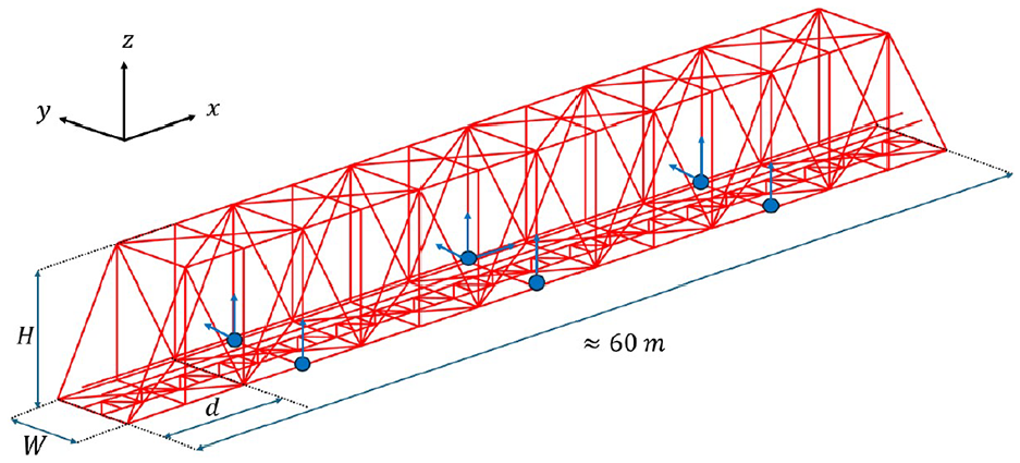
3D FE model of the truss bridge under analysis (H = 7.70 m, W = 5.25 m, and d = 8.64 m).
The structure is characterised by ideal hinge and roller boundary conditions, with a ballastless track. Euler-beam elements were used to create the model, each with six degrees of freedom per node. This modelling choice is based on the fact that the beams in question are slender. Moreover, the elements of this structure predominantly work under axial forces. Since the FEM model reflects the centrelines of the beams, the moments at the nodes are not significant. Therefore, it is possible to model the connections between the bridge elements either using hinges or rigid connections, expecting no significant changes. The geometrical properties of the model were derived from previous field surveys and technical drawings related to the long span of the bridge. The steel material in the model is assigned a Young’s Modulus of 200 GPa, a Poisson’s ratio of 0.3, and a density of 7850 kg/m3. The density was artificially increased by 15% to account for elements not included in the calculation of the net cross-sectional area of each truss member, such as bolts and connecting plates. Additionally, concentrated masses were applied to the bridge deck to represent non-structural components like timber sleepers, track plates, handrails, and footbridges along the sides of the bridge. Proportional damping is assumed in this work (i.e. Rayleigh model72,73):
Comparison between experimental and numerical frequencies for the first seven mode shapes of the bridge.

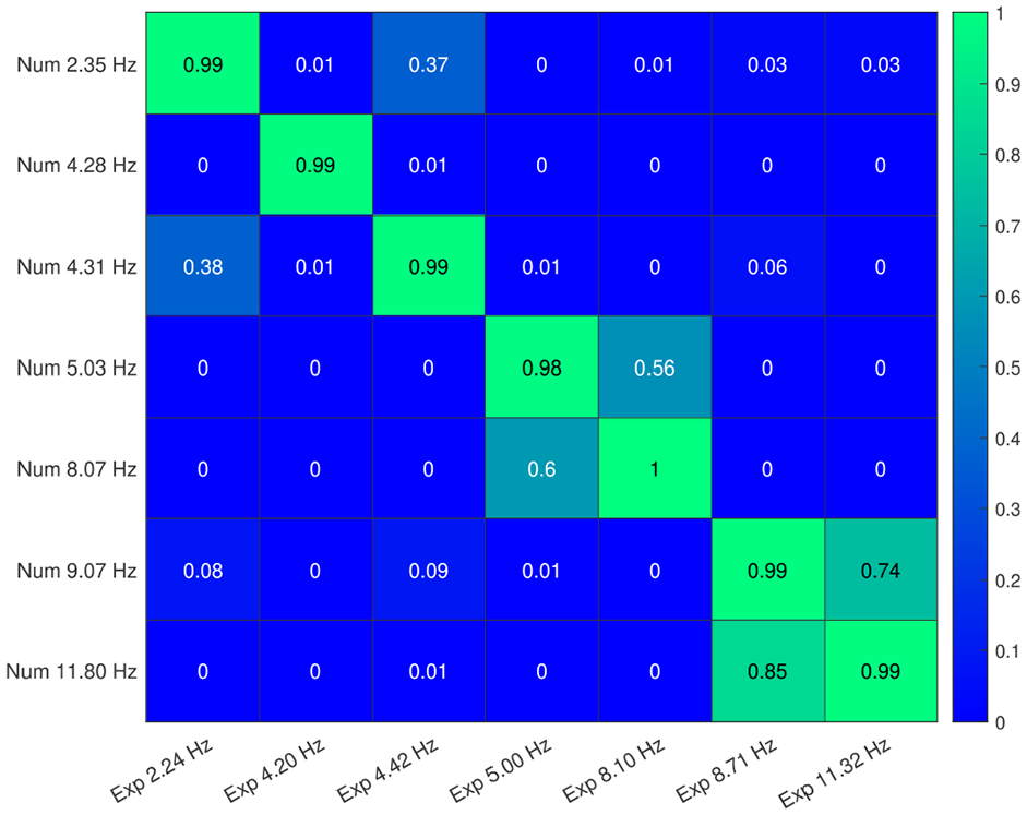
MAC matrix for the first seven modes of the bridge under analysis.
Train-track-bridge dynamic interaction
As mentioned before, the simulation of train-track-bridge (TTB) dynamic interaction is conducted using ADTreS. 59 This software facilitates finite element (FE) modelling of track and bridge structures, offering flexibility in selecting different FE element types, such as Euler beam, plate, or bar elements. As mentioned before, the rail vehicle is instead modelled using a multibody approach.
Structure and train are modelled as two different sub-systems, coupled by contact forces. Structure equations of motion can be written in the following way:

where
Considering the generic i-th vehicle, the following equation can then be written:

where
Therefore, the coupling between the train and the track-bridge structures is achieved through contact forces exchanged at the wheel-rail interface, where a multi-Hertzian 79 wheel-rail contact model is applied. Prior to simulation, using either measured or theoretical wheel and rail profiles, the necessary parameters for calculating the contact forces are stored in a contact table. 63 As reported in Alfi and Bruni, 62 after having computed wheel-rail relative displacements and velocities in all potential contact points, it is possible to enter the contact table with the relative wheel-rail displacement and the longitudinal position. Key contact parameters, stored in the contact table, include the contact angle, wheel’s rolling radius, local curvature radii of the wheel and rail profiles.62,63,65
Considering the m-th wheel, the normal component of the contact force in the q-th potential contact, is computed according to the following set of equations:

where
Once longitudinal and lateral creepages are calculated according to the expression in Alfi and Bruni, 62 longitudinal and tangential contact forces are derived using the Shen, Hedrick, and Elkins formulation. 80 Then, lagrangian components of the contact forces on wheelset and track free coordinates are evaluated.60–62 ADTreS supports multiple simultaneous wheel-rail contact points, with the option to include both new and worn wheel-rail profiles and to account for track geometrical irregularities. Time integration is carried out using the Newmark integration method, with a modified time-step procedure to handle the nonlinearity of the contact problem,62,65,73 as schematically depicted in Figure 5.

Time-integration scheme to handle contact non-linearities.
More in detail, assuming a forward motion of the rail vehicle, with constant speed V, the longitudinal position of the m-th wheel

where
At the beginning of the generic j-th time step, the first approximation (p = 1) of the contact point motion is calculated, considering the wheels in the new position. Once the contact forces are calculated, after having computed the generalised contact forces, equations (1) and (2) are integrated. Then, a new approximation (at p = p + 1) of the contact point motion is obtained and the contact forces are calculated again. Therefore, an iterative procedure is performed (green dashed box in Figure 5) within the j-th time step. Once convergence is reached for the contact forces, the time step can be then incremented. 81
For further details on the simulation software, please refer to References 59, 62, and 63.
Damaged scenarios
The simulated damage scenarios, considered in this study, all pertain to corrosion, the primary cause of material degradation in steel structures. Corrosion is a natural electrochemical process in which metals react with their surrounding environment. In steel structures, this process leads to a reduction in the cross-sectional area of the affected elements, compromising their structural integrity and performance. 82 In this work, corrosion is simply modelled as a reduction of the same quantity of both density and Young modulus to account for flexural and axial stiffness reduction as well as material loss. This modelling choice is equivalent to a reduction of the cross-sectional area, which causes a decrease of the resistance of the chord and its mass. As assumed by Simoncelli et al. 82 and Xiao et al., 83 this damage affects the whole extension of the flawed element. A set of scenarios is considered in this work, as schematised in Figure 6. Three levels of damage were modelled, namely 15, 25, and 50%, while the damage was applied to two distinct members (one at a time), that is, cross-girders and stringers. In case of damage SD (applied to stringers), both the two stringers are degraded of the same quantity: in this damage scenario, two different locations are investigated (i.e. subscripts 2 and 3). Instead, for damage type CG (applied to cross girder), three positions were considered (i.e. subscripts 1, 2, and 3), to investigate the effect of damage position on the detection algorithm.

Top view of the bridge deck. Damages scenarios are highlighted in the figure, concerning cross girders and stringers.
Plan of simulations
The methodology presented in this work was tested considering variations in terms of operational variables. To this end, the authors acted on the following features:
train mass;
track irregularity;
travelling speed.
In particular, five different configurations of the same convoy were used, changing carbody masses to account for different passenger traffic levels during the day. A comparison between numerical axle loads for the adopted vehicles and the experimental counterpart consisting of a sample of 268 trains of the same typology is shown in Figure 7. Track irregularity was changed to model its evolution in time, among different vehicle transits. This was done, starting with the generation of one reference longitudinal profile obtained as a random phase spatial realisation of the PSD curve defined by ORE B176, 84 considering “low level” defects. Then, other four profiles are constructed starting from the reference one. To do so reference amplitudes and phases are increased of a quantity whose maximum depends on the spatial frequency range under analysis: 5% for spatial defects larger than 3 m, and 10% for spatial defects lower than 3 m. This procedure aims to model the differential evolution of track irregularity, which is assumed to evolve faster for lower defects than larger. As mentioned before, train’s mass variations are considered as well, with five different train convoys used for the simulations. Furthermore, the modelled vehicles move with a forward speed ranging from 80 to 130 km/h. Therefore, the simulated scenarios account for a large variability of inputs other than the occurrence of a damage, whose detection is the target of the presented methodology.

Axles load for the five passenger trains considered in the simulations set (train 1–5). Solid red line describes the mean value for each axle load of the convoy, measured on a population of 268 corresponding real train passages. Blue dashed lines define
Methodology
This section is dedicated to the presentation of all the steps of the developed damage detection methodology, starting from the raw data consisting of vertical bogie accelerations. As highlighted in the introduction, the authors concentrated on exploring the feasibility of using a single sensor, installed on the leading bogie of the train, to evaluate the health condition of a Warren truss bridge. The ability to rely on one single sensor, to detect the presence of structural damage across the bridge deck, presents significant potential in terms of cost-efficiency, offering a highly advantageous alternative when compared to more complex direct monitoring systems. The presented methodology relies on the following main steps:
CWT applied to leading bogie vertical acceleration. To do so, a complex Morlet wavelet is adopted and set according to Fitzgerald et al. 28 ;
Identification of the frequency range of interest, given the dimension of the bridge module (of length d) and the travelling speed, which together define the passing frequency
Averaging of the absolute values of the obtained wavelet coefficients along frequency dimension, in the band of interest;
Resampling over space dimension of the curve obtained in the previous point;
Adoption of a sparse autencoder (SAE) used to encode and decode the obtained CWT curve;
Presentation of two different damage indices: the first is based on Hotelling’s distance applied to the latent space, while the second is simply the signal reconstruction error measured by MAE.
Each point introduced before is illustrated in Figure 8, and explained in detail in the following sections. Please notice that the bogie vertical acceleration time series, as well as its CWT scalogram, are plotted between two specific time instants. Precisely, the time at which the first axle of the “instrumented bogie” enters the bridge and the time where its second axle exits it. To move from time to space domain, the travelling speed must be considered, assumed to be constant. This means that the spatial window of interest (whose length is

Representation of the damage detection algorithm flow chart.
Signal processing: CWT
For each considered scenario, the obtained vertical bogie acceleration is processed through 1D Continuous Wavelet Transform (CWT). 85 The latter offers several advantages compared to Fast Fourier Transform 86 when processing and analysing time series with the purpose to extract damage-sensitive indications. In fact, CWT provides a time-frequency representation of the processed signal, allowing the analysis of its frequency content as well as how it evolves with time. Instead, FFT provides the user only with frequency information without retaining any time localisation capability. Therefore, FFT is generally less effective in the identification of damages which are localised in space (i.e. in time). Moreover, CWT is inherently more suitable for the processing of non-stationary signals and it also allows for multi-resolution analysis. This is possible provided that wavelet atoms can be translated in time and dilated 85 in shape: this aspect clearly enhances the detection of damages that can manifest their effects at different frequencies.
In this work, a complex Morlet wavelet is considered to perform CWT operation on vertical bogie accelerations. This family of wavelets is described by the following equation:
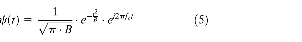
where two input parameters can be clearly distinguished, namely the bandwidth B and the centre frequency
For the present study, the authors opted for the same centre frequency and bandwidth used by Fitzgerald et al.,
28
given their promising results for the detection of scour defects. Therefore, a bandwidth B of 1 was assumed, together with a centre frequency

where

Process to obtain
Autoencoders architecture and preprocessing
Sparse Autoencoder (SAE) is a variation of the conventional autoencoder, specifically designed to learn sparse representations of data, emphasising the extraction of the most distinctive features. The SAE achieves this by introducing a sparsity constraint during training, which encourages the model to encode only the most relevant information while ignoring unnecessary details. 92 This feature results in a more efficient and focused representation of the data, helping the model distinguish between significant patterns and background noise.
During the training process, differently from a Convolutional autoencoder (CAE), the SAE incorporates a sparsity penalty term

where x is a vector representing the network inputs,
By enforcing sparsity, the SAE enhances the model’s ability to highlight fundamental characteristics of the data, making it more effective at identifying structural changes or anomalies. 21 The sparsity constraint reduces the risk of overfitting by preventing all neurons from being activated simultaneously, making the model more effective for unseen data. Moreover, it enforces compact feature representations, making them beneficial for high-dimensional data analysis and reducing computational costs.
In this work, two different neural networks (NNs) are employed, distinguished by the type of input they receive: the first network, hereafter called

where
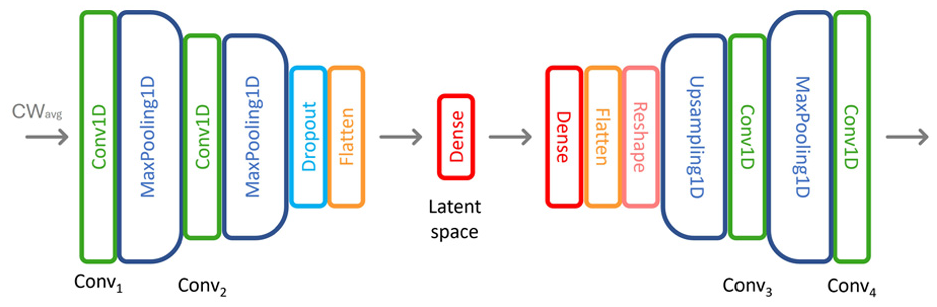
Schematic representation of the first network without considering train velocity, called

Schematic representation of the second network, which considers train velocity, called
Damage detection: Batch reconstruction error
The reconstruction error used to assess the presence of damage is the Mean Absolute Error (MAE), as defined in equation (9):
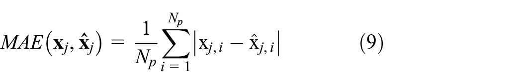
where

This approach ensures that the damage index accounts for multiple signals (multiple runs), providing a more reliable estimate of the damage level. In this work, the original signal
Damage detection: Hotelling’s
control chart
By means of Hotelling’s
In this study,
In particular, considering a matrix

where r is an integer parameter referred to as subgroup size that determines the
Results
Bayesian optimisation
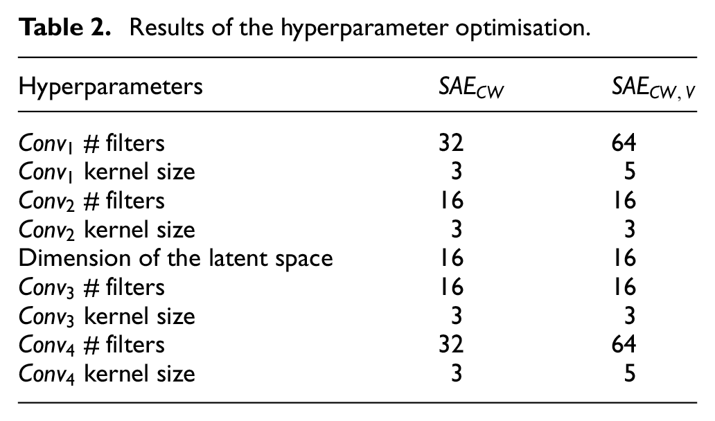
To identify the best combination of hyperparameters, a sensitivity study is conducted involving multiple trials. Optuna 96 is employed to utilise sampling algorithms like the Tree-structured Parzen Estimator (TPE) for selecting hyperparameter sets to be evaluated. The TPE algorithm is particularly effective for high-dimensional optimisation problems and efficiently navigates complex search spaces. A total of 200 trials are conducted for each analysis, where each selected hyperparameters set is used to train and evaluate the model. An objective function is defined to measure the model’s performance based on the chosen hyperparameters, specifically by minimising the reconstruction error of the NN. As trials progressed, Optuna adjusts its sampling strategy to concentrate on areas of the search space likely to yield optimal hyperparameters. After completing 200 trials for each analysis, Optuna identifies the best hyperparameters combinations. It optimises the following parameters with a given set of possible values:
Number of convolutional filter of
Kernel size of
Number of convolutional filter of
Kernel size of
Dimension of the latent space: start: 8, step: 8, end: 64.
Number of convolutional filter of
Kernel size of
Number of convolutional filter of
Kernel size of
This optimisation is run for each network by considering ADAM optimiser on a training process of 1000 epochs and implementing a early stopping callback on validation loss of 30 epochs. The best hyperparameters obtained are resumed in Table 2.
Results of the hyperparameter optimisation.
Damage detection
The sparse autoencoder (SAE) is trained considering a total number of 760 simulations over the healthy structure, accounting for variability in terms of vehicle mass, speed, and track irregularity. The training set comprises 80% of the healthy bridge simulations, while both the validation and testing sets each account for 10%. The autoencoder is trained to encode the input

Original
As previously introduced, two architectures were considered for the SAE neural network (NN), where the second accounts for vehicle speed, whose information is directly fed into the latent space (see Figure 11). For this second case, the performance of the
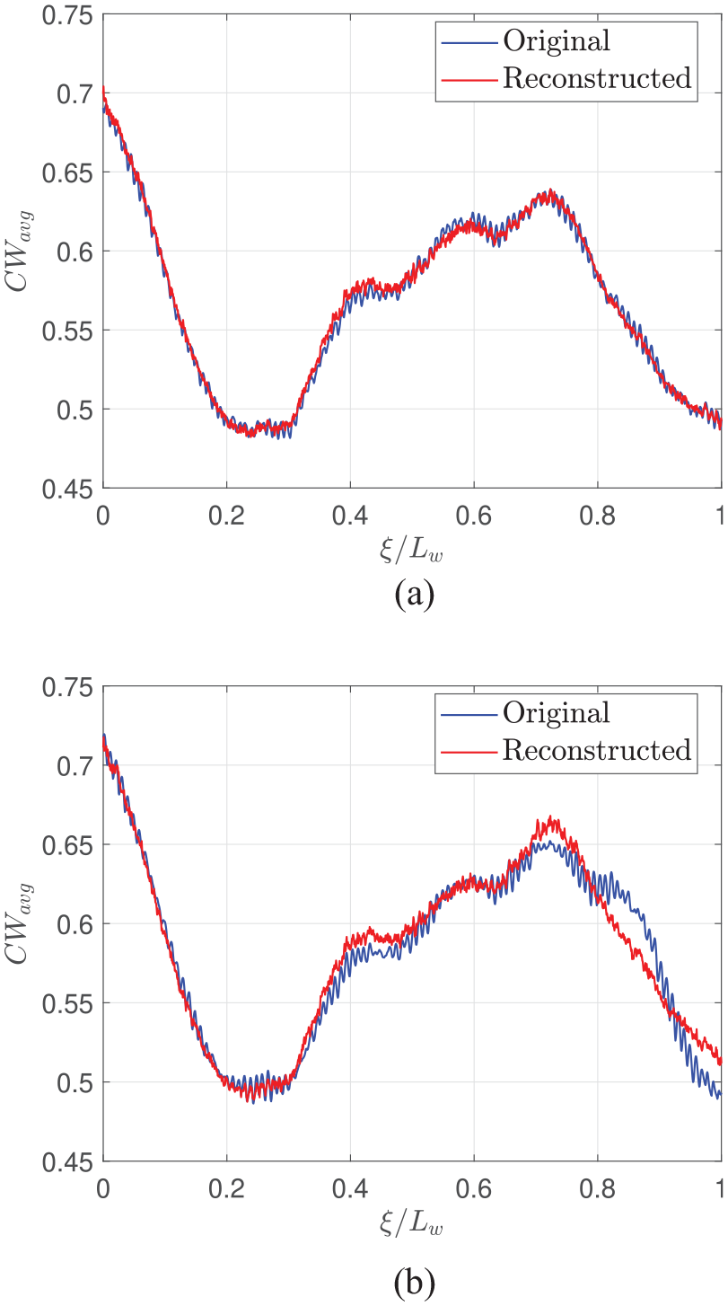
Original
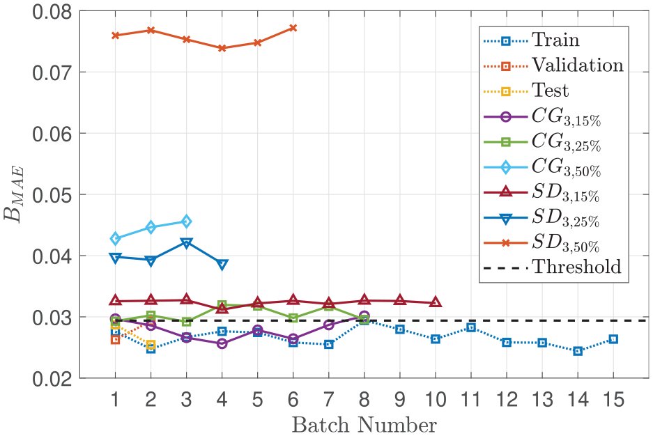
In this work, the objective is to investigate the feasibility of adopting single or multiple train transits to detect damage occurrence across bridge span. It is important to stress the following aspect: for each degraded scenario, simulations are carried out considering operational variables presence (considered also in healthy case), and, before grouping different train transits together, they are automatically shuffled. This means that each batch of train transits, referred to a specific damage scenario, contains a set of bogie vertical accelerations that was randomly extracted from the whole dataset concerning that specific damage. An important aspect to consider for damage detection is the number of train runs that are necessary to detect the onset of a damage. To this end, damage

where TP refers to the number of true positives, TN to true negatives, while FP and FN are respectively the number of false positives and negatives identified by the presented damage index. In particular, while Figure 14(a) refers to the

Accuracy of the damage detection algorithm as a function of train batch size: (a)
For the considered scenario, the
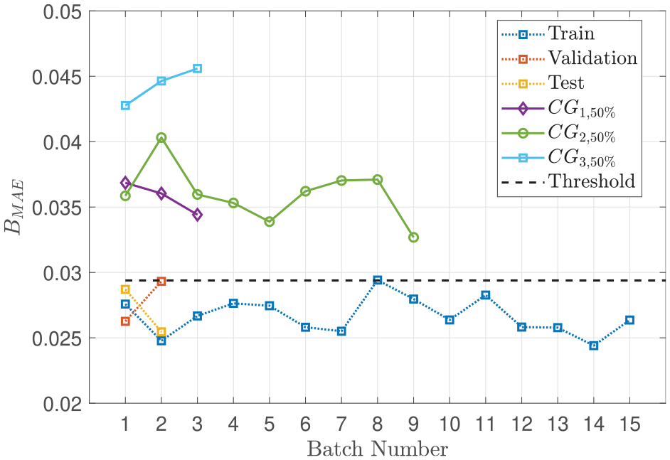
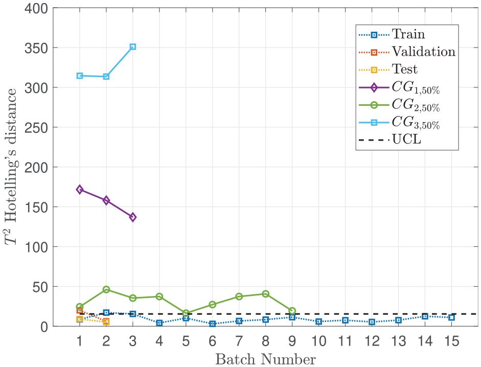
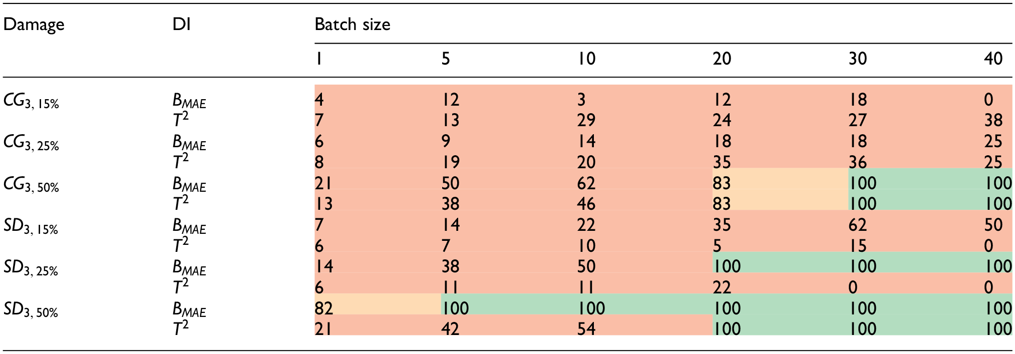
Going more in detail with the damage detection indices, Figure 15 shows the

Accuracy performance for the two damage indices, as a function of considered scenario and the batch size. Two damage types and three different intensities are considered. The adopted NN architecture is


For accuracy larger or equal to 95% the shading colour is green. For values between 94 and 81 is orange. Finally, for values lower than 81, the colour of the shading is red.
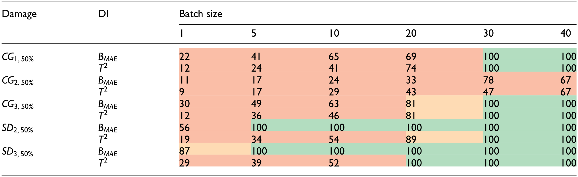
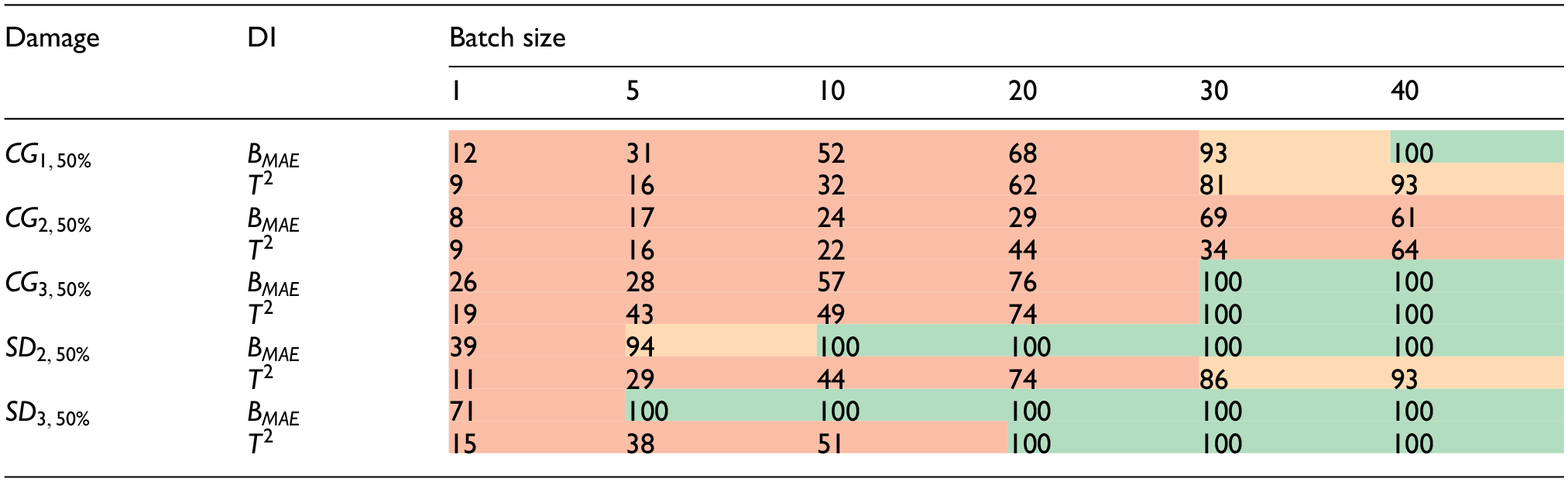
According to Figure 6, different damage positions were modelled in this work, for both CG and SD damage scenarios. This was done in the attempt to investigate any influence played by damage position over DI magnitude. Focusing on damage affecting cross girders, Figures 17 and 18 report the results in terms of
Accuracy performance for the two damage indices, as a function of considered scenario and the batch size. Two damage types, different positions, and same intensity are considered. The adopted NN architecture is


For accuracy larger or equal to 95% the shading colour is green. For values between 94 and 81 is orange. Finally, for values lower than 81, the colour of the shading is red.
Robustness to velocity error and measurement noise
To check and investigate damage detection performances in scenarios closer to real-working conditions, two other factors are taken into account in this section. One is the measurement noise, modelled according to the approach employed by de Souza et al. 36 and Sarwar and Cantero. 50 Therefore, a random artificial noise is added to the vertical bogie accelerations, with the following expression:

where
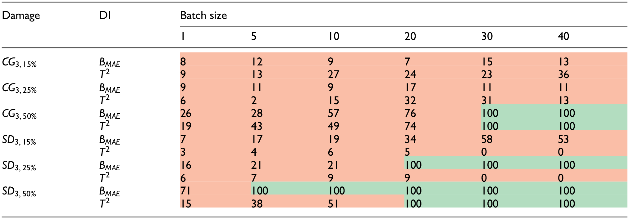
Accuracy performance for the two damage indices, as a function of considered scenario and the batch size. Two damage types and three different intensities are considered. The adopted NN architecture is
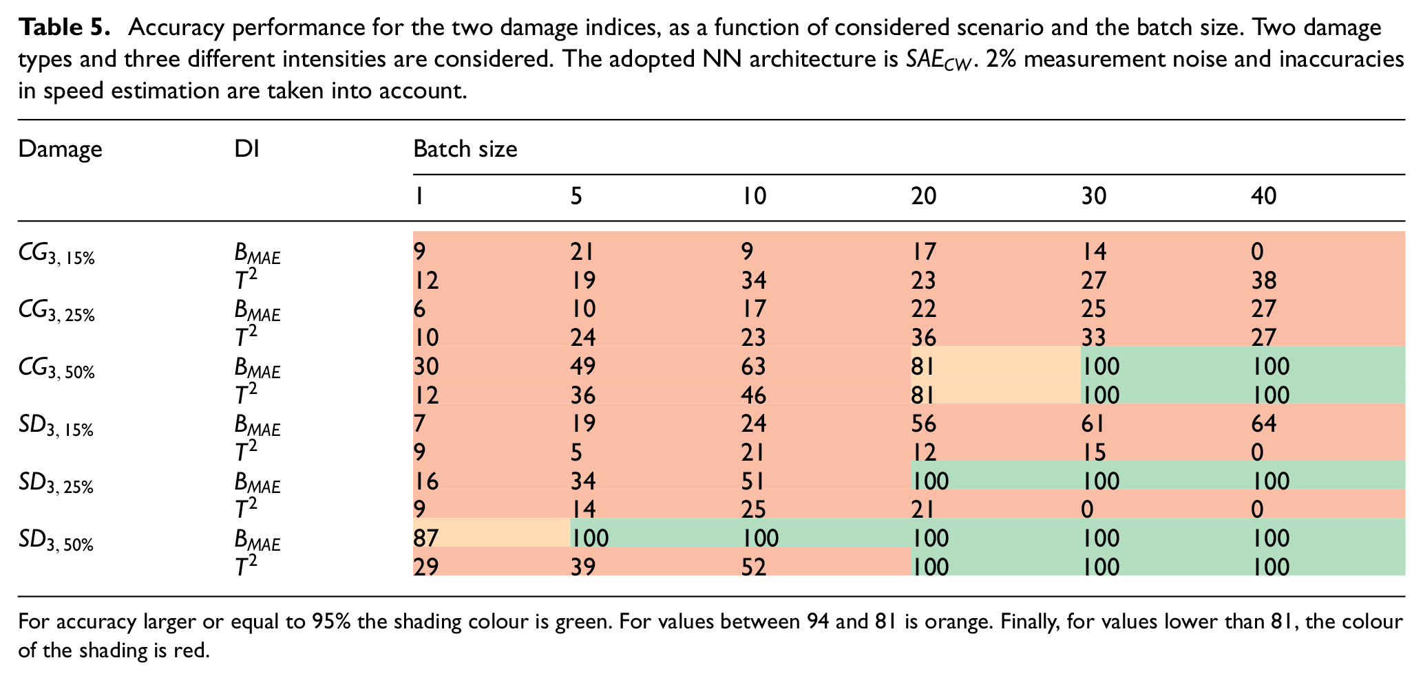

For accuracy larger or equal to 95% the shading colour is green. For values between 94 and 81 is orange. Finally, for values lower than 81, the colour of the shading is red.
Table 6 is the dual of Table 4, again, considering the addition of
Accuracy performance for the two damage indices, as a function of considered scenario and the batch size. Two damage types, different positions, and same intensity are considered. The adopted NN architecture is

For accuracy larger or equal to 95% the shading colour is green. For values between 94 and 81 is orange. Finally, for values lower than 81, the colour of the shading is red.
For the case featured by a measurement noise of
Accuracy performance for the two damage indices, as a function of considered scenario and the batch size. Two damage types and three different intensities are considered. The adopted NN architecture is

For accuracy larger or equal to 95% the shading colour is green. For values between 94 and 81 is orange. Finally, for values lower than 81, the colour of the shading is red.
Accuracy performance for the two damage indices, as a function of considered scenario and the batch size. Two damage types, different positions, and same intensity are considered. The adopted NN architecture is


For accuracy larger or equal to 95% the shading colour is green. For values between 94 and 81 is orange. Finally, for values lower than 81, the colour of the shading is red.
Accuracy performance for the two damage indices, as a function of considered scenario and the batch size. Two damage types and three different intensities are considered. The adopted NN architecture is

For accuracy larger or equal to 95% the shading colour is green. For values between 94 and 81 is orange. Finally, for values lower than 81, the colour of the shading is red.
Accuracy performance for the two damage indices, as a function of considered scenario and the batch size. Two damage types, different positions, and same intensity are considered. The adopted NN architecture is

For accuracy larger or equal to 95% the shading colour is green. For values between 94 and 81 is orange. Finally, for values lower than 81, the colour of the shading is red.
Based on the results shown in this section, a set of considerations can be drawn: the authors have developed a robust damage detection algorithm utilising Continuous Wavelet Transform (CWT) and sparse autoencoder (SAE) NN. Compared to de Souza et al., 36 where the authors use a SAE-based damage detection algorithm, the present paper requires only one single sensing point rather than multiple ones. In fact, the proposed methodology allows for the identification of defects using a single sensor mounted on the leading bogie of the heading coach, which, compared to techniques developed in other studies,51,52,54 potentially results in significant cost savings.
The study focuses on a steel truss structure, a structural archetype not extensively discussed in the related literature. In fact, according to the authors’ best knowledge of past researches in this field, only the study, proposed by the authors in Bragança et al., 55 presents a damage detection technique exploiting CWT and autoencoders applied to a Warren truss bridge. In relation to that work, the approach proposed in this paper involves a passenger train instead of a freight train, requires the use of only one sensor (instead of eight), and is demonstrated to be effective at higher speeds (i.e. up to 130 km/h instead of 60 km/h). Then, compared to other works, such as Fitzgerald et al., 28 the frequency band of interest is chosen based on the structural conformation which is typical of the bridge under analysis as proposed by Bernardini et al.. 91 In this study, the authors also explored the use of a Damage Index (DI) based on features contained in the latent space, rather than focusing on the decoder output, differently from what has been done in other works, including References 36, 51, 52, and 55. Finally, under this regard, according to authors’ best knowledge, this work represents the first application of the concept of Hotelling’s distance for latent space features distributions in the field of drive-by bridge monitoring. Further insights are critically discussed in the conclusions section, outlining main achievement and limitations.
Conclusions
In this work, the authors focused on the definition of a damage detection approach based on Sparse Autoencoder (SAE) and wavelet coefficients, which exploits one single measurement point to detect corrosion damages affecting a Warren truss bridge. Vertical accelerations of the first bogie of the leading coach are processed through Continuous Wavelet Transform (CWT) considering complex Morlet as the mother wavelet. The obtained scalogram was then reduced to a portion of interest defined in the frequency range given by the train forward speed and the module length of the bridge. In this frequency band, the absolute values of the obtained wavelet coefficients are averaged and interpolated in space. This curve represents the input to a SAE NN architecture, whose parameters were defined through Bayesian optimisation, trained to learn to decompose and recompose the input signal. Two NN configurations were modelled and trained in this work, not incorporating or incorporating train speed, that was considered at the latent space level. Two different damage indices (DIs) were proposed: one consisting of the batch Mean Absolute Error (
When dealing with perfect speed and position estimations, the work led to the following main results:
accounting for train speed information at the latent space level does not lead to a more effective SAE NN with improved accuracy performances;
the proposed DIs are found to be both very accurate when dealing with batches of 40 trains and damage intensities equal to
considering the lightest modelled lightest modelled damages,
the presented DIs are sensitive to damage intensity: an increase of damage intensity reflects in a larger magnitude for both the DIs;
when considering damages affecting cross girders, highest DI magnitudes are obtained when the flawed element is closer to the end of the bridge;
T2 distance appears to be strongly dependent on the position of the damaged cross girder.
In this work, the authors also accounted for three different levels of measurement noise (
Globally, methodology performances decrease, still showing promising results, when dealing with 50% corrosion damages;
When keeping speed and position estimation inaccuracies constant (i.e.
BMAE index appears to be more robust than
Despite the previous point, using both of the two DIs is deemed to be a robust choice that does not require any additional implementation and/or computational costs.
While promising results are achieved, it is worth mentioning that the presented methodology has some limitations, among which, the most complex to be tackled regards the need for a robust and accurate estimation of the forward speed as well as train position, which is crucial for a proper identification of the spatial window of interest. In addition, while relying on one single sensor has several advantages in terms of costs, it may result less robust, due to lack of redundancy of the measuring solution. Finally, it is worth stressing that since this approach exploits the modular conformation which is typical of Warren truss bridges, another choice on the frequency range of interest must be carried out when dealing with other bridges. Some possibilities can be found in literature, for example, References 24, 27, 28, and 51. However, the obtained outcomes pointed out the promising performances of the presented methodology, which requires only one sensor to be installed on the train, representing a significant advantage in terms of costs, if compared to direct systems and to other drive-by approaches relying on sparse autoencoders. Future outlooks will consist of combining the developed methodology with the adoption of more than one sensor. Moreover, the effect played by module length and speed estimation errors, without any position estimation inaccuracy, will be investigated.
To further explore the potential of sparse autoencoders, future research can focus on integrating sparsity with additional regularisation techniques such as variational methods to enhance performance. Another promising direction is the combination of sparse autoencoders with generative models, such as GANs, to improve latent space representations.
Footnotes
Handling Editor: Chenhui Liang
Funding
The author(s) received no financial support for the research, authorship, and/or publication of this article.
Declaration of conflicting interests
The author(s) declared no potential conflicts of interest with respect to the research, authorship, and/or publication of this article.
Data availability statement
The data that support the findings of this study are not openly available due to reasons of sensitivity. Some of the data are available from the corresponding author upon reasonable request.