Sage Journals: Discover world-class research

Abstract

Heat damage in automobiles is concentrated in the engine compartment, where the radiator is key to cooling performance. The relative positions of the intercooler, condenser, and oil cooler also influence this performance. This study optimizes the positions of these cooling components in a mid-sized pickup truck to address heat damage. Vehicle tests first identified extreme working conditions leading to heat damage. Computational fluid dynamics (CFD) simulations then analyzed heat damage locations and assessed the impact of component positions. A near-orthogonal Latin hypercube method selected layout schemes, and a Chebyshev transformation improved their spatial distribution. Parametric modeling and CFD simulations of the thermal field were conducted. Based on simulation results, a multi-objective two-layer deep Gaussian process model predicted heat source temperatures. The positions of cooling components were optimized using a genetic algorithm with heat-sensitive locations as the objectives. The results showed temperature reductions at all four critical positions, with the urea injection pipe temperature decreasing by 10.2°C. This approach effectively mitigates heat damage in the engine compartment and can be applied to optimize cooling component layouts in pickup trucks.

Keywords

automotive thermal management deep Gaussian process aerodynamic layout heat damage engine cooling system

Introduction

Owing to high engine power and harsh operating conditions, the thermal load of the engine compartment in mid-sized pickup trucks is significantly greater than that of urban household cars under typical driving conditions.¹ Fifty percent of vehicle malfunctions are caused by engine-related issues, with the majority of engine failures being associated with thermal damage. A common type of thermal damage is the rapid local temperature rise of components caused by insufficient heat dissipation performance in the engine compartment under various adverse operating conditions. Therefore, the heat dissipation performance of engine cooling systems is subject to increased demands,² and improving heat dissipation performance is crucial for addressing thermal damage problems.

Owing to the long duration and high cost of full-scale vehicle testing, computational fluid dynamics (CFD) simulation methods are widely used to investigate the flow and temperature fields in automotive engine compartments.^3,4 However, current methods for addressing thermal issues in engine compartments focus primarily on improving the structure and parameters of cooling components. Zhan et al.⁵ researched automotive air conditioning condensers and reported that reducing the fin spacing effectively improved the condenser performance. Pingping and Zhendong,⁶ in response to the significant recirculation issue in the engine compartment, proposed four optimization schemes: arranging sealed air guiding channels, tilting the cooling module by 5°, centrally positioning the cooling fan, and employing dual cooling fans. These solutions effectively improved the heat dissipation performance of the original engine compartment. Zhang et al.⁷ utilized the Cheb-OLH sampling method and surrogate models to optimize the stagger angle, sweep angle, and chord of a cooling fan, thereby increasing the fan cooling efficiency. Tang et al.⁸ replaced the straight bumper beam of an SUV with a U-shaped beam, increasing the airflow to each heat exchanger and enhancing the heat dissipation performance of the exchangers.

Since most automobile manufacturers now rely on finished cooling components provided by suppliers, they are limited to a selection of predefined models. The performance of existing cooling components varies across different vehicle models, resulting in differing effectiveness in addressing engine compartment thermal issues. To achieve optimal performance in specific vehicle models, a comprehensive and scientific method for selecting the optimal installation positions of cooling components is needed.

To explore optimal design solutions, a combination of surrogate models and intelligent optimization algorithms is commonly used. Common surrogate models include the polynomial response surface model (RSM),¹⁰ the neural network model (NN),¹¹ the radial basis function (RBF),¹² the kriging model, and its various derivatives. Owing to their ability to assess uncertainty in predicted results, kriging-related methods have been widely applied in engineering.¹³ However, to provide uncertainty assessments, the kriging model relies on the assumption of second-order stationarity; that is, a stationary stochastic process is predefined.¹⁴ If the autocorrelation function is modeled as Gaussian, this assumption is reflected in the invariance of the mean μ and variance σ. In reality, stochastic processes are not necessarily stationary, and the probability density function may change with variations in dimension and spatial region. Unlike the kriging method, the Gaussian process (GP) also assumes a Gaussian distribution but does not require the mean and autocorrelation functions to remain constant. By further combining GP with deep learning networks, Damianou¹⁴ and Lawrence and Moore¹⁵ proposed the deep Gaussian process (DGP), which retains the flexibility of GP and leverages the enhanced capabilities of deep neural network architectures. This approach results in a more powerful model with improved uncertainty prediction.^17,18 The DGP model has significant advantages in handling complex nonlinear function relationships,¹⁹ adapting to various data distributions, and providing uncertainty assessments for predicted outcomes.²⁰ On the basis of fluid simulation results, this paper employs the DGP model to mine data through a dual-layer GP, establishing high-dimensional visualization techniques that accurately and comprehensively express the mapping relationship between the layout of cooling components and the temperature of the thermal heat-harm position. This method “traverses” all feasible layout schemes to explore the impact of the spatial coordinates of the cooling components on the temperature of the thermal heat-harm position. First, the nearly orthogonal Latin hypercube (NOLH) sampling method²¹ is used to generate the initial experimental design points, which are then transformed via Chebyshev polynomials²² to generate new experimental design points. Second, the vehicle model is then parameterized, corresponding geometric models are created, and mesh generation is conducted. Third, simulation software is used to perform aerodynamic simulations of the internal flow field of the engine compartment, obtaining the temperature distribution within the compartment. Fourth, on the basis of the simulation results, a DGP model²³ is constructed to predict the objective function values, and a genetic algorithm is employed for multiobjective optimization design. Last, high-dimensional parametric visualization techniques based on self-organizing maps (SOMs)¹⁵ are used to analyze the optimization results, providing optimized solutions for the rational layout of cooling components. The significance of this research lies not only in improving engine cooling performance but also in providing an intuitive presentation of complex layout problems under multifactor coupling. This research offers a theoretical foundation for similar layout analysis and decision-making problems in aerospace and other engineering fields.

Therefore, based on fluid simulation results, this paper adopts the deep Gaussian process model to mine data through a dual-layer Gaussian process and constructs high-dimensional visualization techniques to accurately and comprehensively express the mapping relationship between the layout of cooling components and the temperature of thermal damage points. This method allows for a systematic “exploration” of all feasible layout schemes, analyzing the impact of the cooling component positions on the temperature of thermal damage points. As a result, it provides a scientific basis for optimizing the layout of cooling components in the engine compartment. The significance of this research lies not only in enhancing engine cooling performance but also in offering an intuitive presentation of complex layout problems under multifactor coupling, providing a theoretical foundation for similar layout analysis and decision-making problems in aerospace and other engineering fields.

Computational fluid simulation model of the engine compartment

Preprocessing of automotive CAD models

The subject of this study is a commercial mid-sized pickup truck. Owing to the large number of components within the engine compartment, geometric model simplifications were applied to insignificant details such as bolts, screws, and small holes that do not affect the global flow field and temperature field in the engine compartment to reduce the computational load prior to conducting CFD simulations. The simplified full-vehicle CAD model is shown in Figure 1 and includes key components that significantly affect the flow field and temperature field, such as the body, powertrain system, cooling system, chassis system, and exhaust system.

Figure 1.

Full-vehicle CAD model.

Different tools were used to process the surface and volume meshes. First, ANSA was employed to wrap the pickup truck model and create the surface mesh. Second, the surface mesh was imported into STAR-CCM+ for quality checks, refinement in specific regions, and computational domain definition, followed by volume mesh generation.

The computational domain was created on the basis of the standard²⁰ for aerodynamic simulation specifications for passenger cars. The domain height and width were each set to seven times the vehicle height and width, respectively, with a front distance more than three times the vehicle length and a rear distance exceeding eight times the vehicle length. Figure 2 presents a schematic of the full vehicle and the computational domain.

Figure 2.

Schematic of the numerical simulation computational domain.

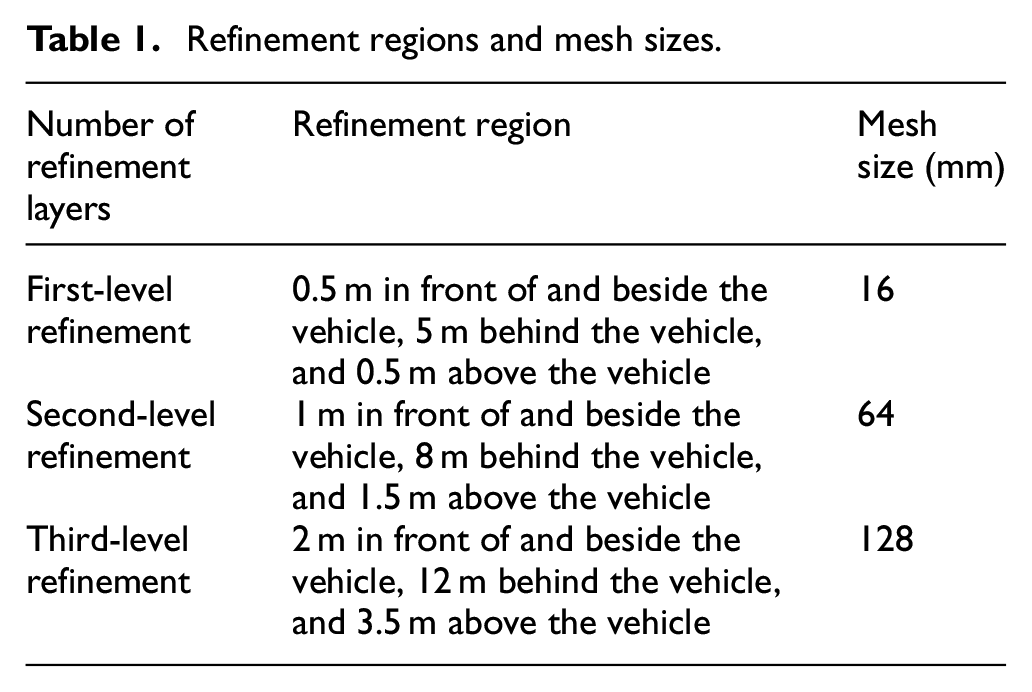
To simulate the flow field conditions inside the engine compartment more accurately, the computational domain was divided into three refinement layers. The refinement regions and mesh sizes are shown in Table 1. Key areas affecting flow, such as the intake grille, engine compartment, and chassis, were locally refined. A schematic of the Y = 0 cross-sectional mesh of the engine compartment after refinement is shown in Figure 3. The total number of tetrahedral meshes for the full vehicle is approximately 55 million.

Table 1.

Refinement regions and mesh sizes.

Number of refinement layers	Refinement region	Mesh size (mm)
First-level refinement	0.5 m in front of and beside the vehicle, 5 m behind the vehicle, and 0.5 m above the vehicle	16
Second-level refinement	1 m in front of and beside the vehicle, 8 m behind the vehicle, and 1.5 m above the vehicle	64
Third-level refinement	2 m in front of and beside the vehicle, 12 m behind the vehicle, and 3.5 m above the vehicle	128

Figure 3.

Schematic of the Y = 0 cross-sectional mesh of the engine compartment.

Boundary condition settings

The boundary conditions for this calculation include a velocity inlet, a pressure outlet, and stationary walls. The specific boundary condition settings are shown in Table 2. The multiple reference frame (MRF) method was used to define the rotating regions for the CFD simulation of the working fan flow field. The multiple reference frame (MRF) method was used to set the rotating region for the numerical computation, with the fan operating at a speed of 2430 rpm and a power of 800 W. The Reynolds-averaged Navier–Stokes (RANS) equations were solved with the k–epsilon turbulence model via the SIMPLE algorithm for pressure correction and second-order upwind discretization.

Table 2.

Boundary condition settings.

Boundary model	Boundary name	Boundary position
External boundary	Inlet	Velocity-inlet
External boundary	Outlet	Pressure-outlet
Internal boundary	Hot engine component	Temperature wall
	Cooling fan	MRF model
	Radiator unit	Porous medium model
	Other unit	Static wall

The thermal boundary conditions involve mainly defining the thermal boundary types and material properties. The high-temperature heat source is assigned a specific temperature, whereas other solid surfaces are defined by their material type, including density, thermal conductivity, and specific heat capacity. To improve the thermal field simulation accuracy within the engine compartment, temperature zones are assigned to the main heat source components. This approach divides the engine surface into five sections and the exhaust pipe into 17 segments. To more realistically reflect the impact of the heat generated by the engine during vehicle operation on the thermal field within the engine compartment and to make the simulation more accurate, the engine is divided based on temperature. The engine surface is divided into five sections, with each section assigned a temperature as a heat source. Additionally, since the exhaust pipe is relatively long and experiences significant temperature differences, it is divided into 17 sections, each assigned a temperature.

In CFD simulations, vehicle heat dissipation components are typically modeled as porous media, which is achieved by defining two parameters—the inertial resistance coefficient and the viscous resistance coefficient—that simulate flow resistance through porous regions. These coefficients are derived from velocity and pressure loss data in the engineering database and fitted into a quadratic function without a constant term, as shown in the following formula:

\frac{Δ P}{Δ n} = \frac{μ}{α} v + \frac{1}{2} ρ C_{2} v^{2}

(1)

where $Δ P$ represents the pressure loss in the direction of the main airflow; $Δ n$ denotes the length of the main airflow, which, in this model, is aligned with the horizontal longitudinal axis of the vehicle and corresponds to the thickness of the heat exchanger; $\frac{1}{α}$ is the viscous resistance coefficient; $C_{2}$ is the inertial resistance coefficient; $v$ is the velocity of the airflow; $ρ$ is the air density; and $μ$ is the dynamic viscosity. The values for both the air density and the air viscosity are provided as experimental data from the manufacturer: $ρ = 1.1108 kg \cdot m^{- 3}$ and $μ = 1.93365 \times 10^{- 5} kg \cdot m^{- 1} \cdot s^{- 1}$ .

The heat dissipation components used in this vehicle include the radiator, intercooler, oil cooler, and condenser. Table 3 provides the inertial and viscous drag coefficients of these components.

Table 3.

Porous media parameters of the heat dissipation components.

Radiator unit	Inertial resistance coefficient (kg/m⁴)			Viscous resistance coefficient (kg/m³ s)
	x	y	z	x	y	z
Radiator	133.46	13,346	13,346	1147.2	114,720	114,720
Intercooler	308.33	30,833	30,833	807.03	80,703	80,703
Oil cooler	210.27	21,027	21,027	890.83	89,083	89,083
Condenser	186.27	18,627	18,627	437.28	43,728	43,728

Experimental testing revealed that under low-speed climbing conditions, the engine compartment temperature reaches its peak, which poses a risk of thermal damage. Consequently, the low-speed climbing condition was chosen for the CFD simulation. The operating conditions were based on vehicle tests: ambient temperature of 40°C, 30% humidity, irradiation intensity of 1050 W/m², vehicle speed of 20 km/h, and slope of 15%. Humidity was adjusted by modifying the air moisture content, and the irradiation intensity was manually set by adjusting the solar load. During simulation, the temperature at potential thermal damage points was monitored, because it varied with each iteration. The temperature criterion was defined as the average temperature with an iterative change not exceeding 1% over 50 steps. However, in several cases, even when the residuals meet the convergence criteria, the temperatures at the thermal damage points continue to fluctuate. This fluctuation was due to the Chebyshev transformation, because certain measurement points were near the boundary of the sampling range. The close proximity of heat dissipation components to other parts in the engine compartment resulted in poor mesh quality. In these cases, the temperature criterion was adjusted to an average temperature with an iterative change not exceeding 3% over 50 steps.

Experimental calibration of the numerical simulations

The components in an automobile engine compartment have complex shapes and multiple performance parameters, making thermal performance evaluation challenging. Traditionally, preliminary designs are completed via empirical methods or engineering estimates and then tested experimentally. The design is iteratively refined on the basis of test results to meet requirements.²¹ With advancements in CFD, combining CFD simulation with experimental testing has become common in aerodynamic design. CFD simulations offer benefits such as low cost, short cycle time, and visualization of flow fields within the computational domain.²² In this study, full-scale vehicle testing, followed by CFD simulations to obtain performance metrics, was conducted. The simulation results were compared with the experimental data to ensure accuracy.

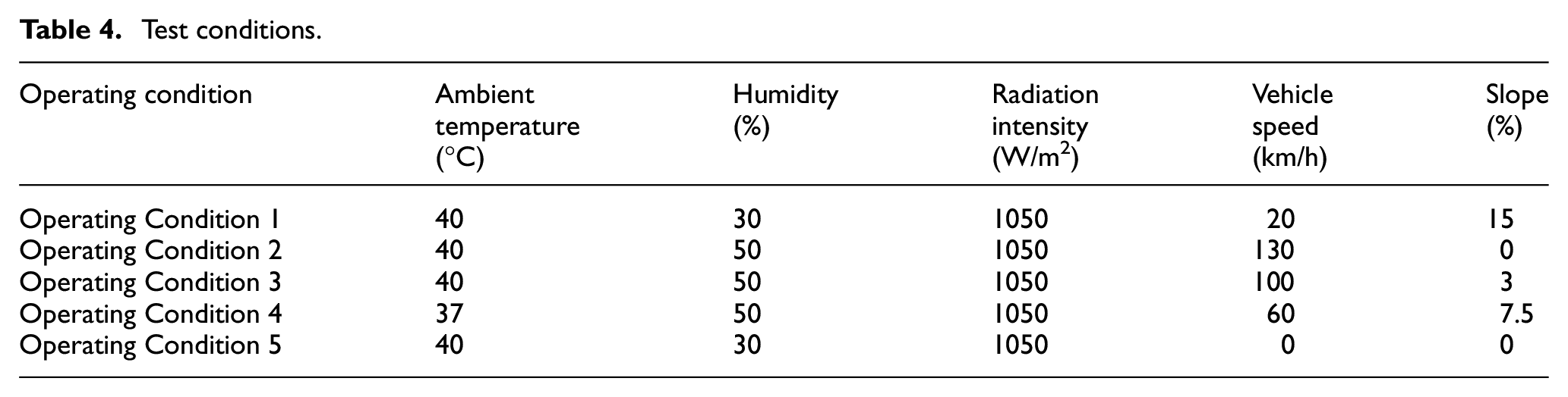
Full-scale vehicle testing was conducted in an environmental simulation chamber following the group standard “Technical Specification for Aerodynamic Simulation of Passenger Cars” to verify the accuracy of the simulation results. The test conditions for the full-scale vehicle experiment are listed in Table 4. Temperature sensors were placed in the engine compartment to measure the temperatures at various points. To establish boundary conditions for the CFD simulations, the primary heat source components were segmented and measured. The exhaust pipe was divided into 17 regions, and the engine components were divided into 5 regions. In the environmental test chamber, the experimental data changes of each temperature and flow measurement point are recorded in real-time, while the airflow distribution at different locations within the engine compartment is also monitored. An infrared thermography device is used to measure the temperature distribution on the engine surface, key thermal damage areas, and within the engine compartment.

Table 4.

Test conditions.

Operating condition	Ambient temperature (°C)	Humidity (%)	Radiation intensity (W/m²)	Vehicle speed (km/h)	Slope (%)
Operating Condition 1	40	30	1050	20	15
Operating Condition 2	40	50	1050	130	0
Operating Condition 3	40	50	1050	100	3
Operating Condition 4	37	50	1050	60	7.5
Operating Condition 5	40	30	1050	0	0

The thermal management system operating data of this vehicle under different driving modes are obtained through experiments. The main experimental data that need to be collected include the following: (1) the coolant flow rate and inlet/outlet temperatures of the engine, radiator, and condenser; (2) the temperature distribution on the surface of the engine and exhaust pipe; and (3) the temperature in heat-sensitive areas. The following shows several temperature measurement test diagrams. Figure 4(a) shows the test points for the urea injection pipe temperature sensor. Figure 4(b) shows the partial test points for the high-temperature exhaust pipe temperature sensor. Figure 4(c) shows the test points for the engine cylinder temperature sensor. The placement of temperature sensors is based on locations that are likely to experience thermal damage according to experience, as well as areas that will be used as boundary condition data in subsequent CFD simulations.

Figure 4.

Test points for the temperature sensor: (a) urea injection pipe, (b) high-temperature exhaust pipe, and (c) engine cylinder.

Analyze the experimental results of the five operating conditions shown in Table 5, which indicate that the temperature within the engine compartment is highest during low-speed climbing under Operating Condition 1, where four heat-sensitive areas were identified. A CFD simulation was conducted for this condition, and the simulated temperatures were compared with the experimental data. The results are presented in Table 6. Discrepancies between the experimental results and the simulated results were observed due to challenges in precisely mapping test point locations in the model and the influence of external factors. However, all the errors were within 10%, which is acceptable for accuracy.

Table 5.

Experimental results.

Operating condition	Turbocharger heat shield (°C)	Urea injection pipe (°C)	Engine compartment wiring harness (°C)	Engine wiring harness (°C)
Operating Condition 1	113.2	119.8	88.7	97.3
Operating Condition 2	109	118.1	88.8	92.2
Operating Condition 3	108.1	117.8	88.6	92.1
Operating Condition 4	108.8	117.8	88.6	91.2
Operating Condition 5	90.3	101.2	84.1	82.7

Table 6.

Comparison of the experimental and simulation results for Operating Condition 1.

Data comparison	Turbocharger heat shield	Urea injection pipe	Engine compartment wiring harness	Engine wiring harness
Test (°C)	113.2	119.8	88.7	97.3
CFD (°C)	102.3	126.7	95	106.1
Error (%)	9.6	5.8	7.1	9

After analyzing the results of the five test conditions shown in Table 5, it was ultimately found that Condition 1 (low-speed climbing condition) resulted in the highest temperature inside the engine compartment, with four heat damage points identified. The insulation material used for both the engine compartment harness and the engine harness is PVC, which is cost-effective and durable but has limited temperature resistance, ranging from −40°C to 105°C. Although the temperatures of these harnesses did not exceed the material’s range during the experiment, they were already very close to the upper limit. Moreover, CFD simulations indicated that the temperature exceeded the allowable range. Considering these factors, it is necessary to reduce the temperature in these areas. The turbocharger heat shield and the urea injection pipe are made of stainless steel, which, as metal components, have high-temperature resistance. However, plastic parts are present around these components. To protect the surrounding plastic parts, the outer surfaces of these metal components need to maintain lower temperatures, making these two locations heat damage points. A CFD simulation was conducted for this condition, and the simulated temperatures were compared with the experimental temperatures, as shown in Table 6. Due to the inability to precisely match the sensor placement in the experiment with the model representation and the presence of external influencing factors, discrepancies exist between the experimental and simulated results. However, all errors are within 10%, which is considered to meet accuracy requirements.

Although experiments were conducted, due to the limitations of the experimental conditions, the infrared thermal imager can determine the temperature distribution but cannot accurately reflect specific temperatures. Additionally, due to the constraints of vehicle disassembly during testing, some temperature sensors could not measure the intended component locations. In such cases, simulations are needed to identify specific thermal hazard locations under extreme conditions, supplementing this missing information. As a complementary tool to experiments, simulations can reduce the number of tests, lower testing costs, and more precisely locate potential thermal hazard areas. Moreover, conducting experiments alongside simulations helps analyze the coupling relationship between the two, calibrate key aspects such as boundary condition settings and mesh division in simulations, and facilitate the accumulation of technology and data.

Analysis of heat-sensitive locations in the engine compartment

The three-dimensional CFD simulation results were postprocessed to obtain the velocity vector diagram and temperature contour plot at the Y = 0 position within the engine compartment.

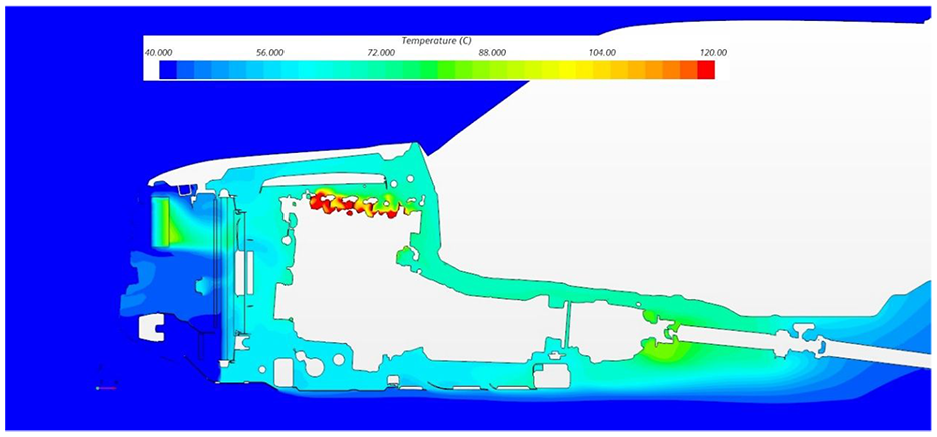
Figure 5 shows the velocity vector diagram. The engine compartment contains numerous components in a compact space, resulting in complex airflow conditions. Only part of the airflow entering from the intake grille flows into the intercooler, whereas the other part bypasses the intercooler and flows directly to the condenser and oil cooler. Owing to the suction effect of the cooling fan, the airflow is accelerated and impacts the engine at high speed, creating a vortex between the fan and the engine and creating a high-temperature region in this area. A small portion of the airflow bypasses the heat-dissipating components and flows directly into the engine compartment, forming vortices above the condenser and below the oil cooler, which adversely affects the heat dissipation performance of the compartment. The temperature distribution within the engine compartment is shown in Figure 6. Under low-speed climbing conditions, high temperatures were observed at the turbocharger heat shield, urea injection pipe, engine compartment wiring harness, and engine wiring harness, causing heat damage at these locations.

Figure 5.

Velocity vector diagram at Y = 0.

Figure 6.

Temperature contour plot at Y = 0.

The distribution of the heat-sensitive points is shown in Figure 7: (a) urea injection pipe and (b) engine compartment wiring harness, engine wiring harness, and turbocharger heat shield. The urea injection pipe is located near the high-temperature exhaust pipe, where the exhaust pipe temperature reaches 340°C, causing the urea injection pipe temperature to increase to 126.7°C. The high temperatures around the engine compartment wiring harness and engine wiring harness are due to their proximity to the engine, generating high-temperature zones, whereas the turbocharger heat shield, located near the catalytic converter, reaches a temperature of 102.3°C.

Figure 7.

Temperature diagram of heat-affected components: (a) in car position and simulation result of urea injection pipe and (b) simulation of other critical heat-harm positions.

Under low-speed climbing conditions, the insufficient intake airflow at the front grille fails to adequately exchange heat with the coolant in the radiator, resulting in suboptimal radiator cooling performance. Additionally, not all of the cold air entering the engine compartment through the grille passes through the radiator for heat exchange; some airflow bypasses it, entering the compartment directly and forming vortices, which reduces the utilization of cold air. Adjusting the position of the radiator and directing airflow paths can increase cold air utilization, which helps reduce temperatures in heat-sensitive areas within the engine compartment.

Engine compartment thermal damage optimization based on deep Gaussian processes

Introduction to the DGP model

Deep Gaussian processes (DGPs) are based on the GP mappings of deep belief networks²³ and are designed to address various complex functional relationships and classification tasks. By modeling the posterior distribution of class labels, DGPs provide uncertainty estimates, improving their ability to address ambiguous samples. The structure of DGPs resembles the hierarchical organization of neural networks, as shown in Figure 8, comprising multiple stacked GPs. The input of each internal GP is governed by the output of the preceding GP, allowing each layer to extract different features. This multilayered architecture enables DGPs to capture complex nonlinear relationships and multiscale structures within data more effectively. The GP controls the mappings between layers, with each mapping corresponding to an individual GP.¹⁵

Figure 8.

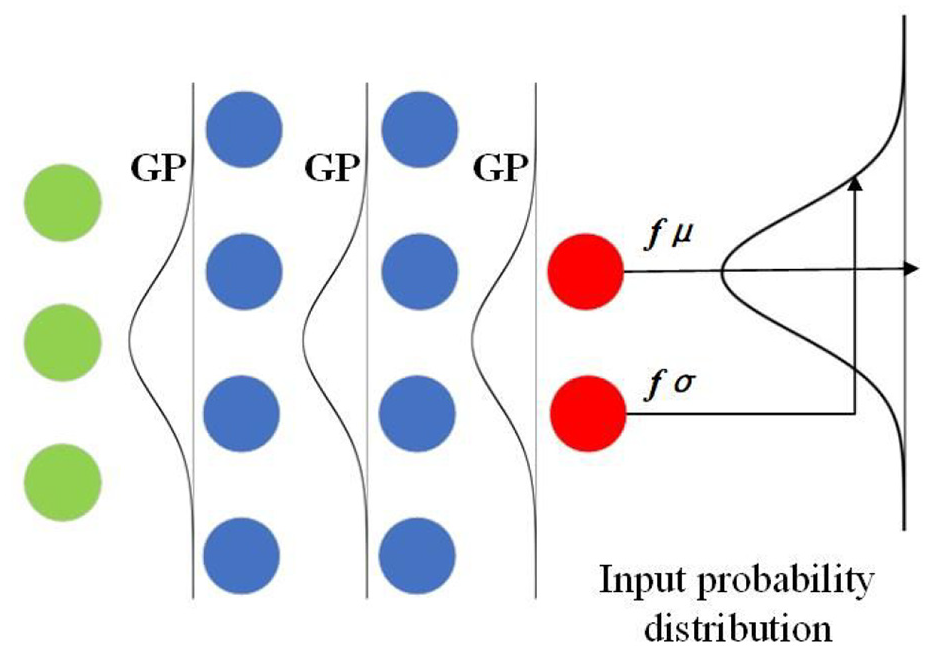
DGP model diagram.

The circles in the diagram represent nodes. Within the hidden layers, each node serves as the output of the previous layer and as the input for the subsequent layer. The mapping relationships between layers are defined via the GP. The results of the DGP are characterized by the output layer through the mean and variance. The DGP model is described as follows:

\begin{matrix} p (Y, {F^{l}, U^{l}}_{l = 1}^{L}) = Π_{i = 1}^{N} p (y_{i} | f_{i}^{L}) \\ Π_{i = 1}^{L} p (F^{l} | U^{l}; F^{l - 1}, Z^{l - 1}) p (U^{l}; Z^{l - 1}) \end{matrix}

(2)

In this equation, $Π_{i = 1}^{N} p (y_{i} | f_{i}^{L})$ represents the marginal likelihood of the DGP, L denotes the number of layers in the DGP, and N is the number of samples. $F^{l}$ denotes the output of layer l, whereas $U^{l}$ represents the inducing variables used to accelerate computation, with $Z^{l - 1}$ indicating the inducing points at layer $l - 1$ . $Y$ is a matrix where the $i$ -th row contains the observed value $y_{i}$ . $f_{i}^{L}$ represents the function value of the $i$ -th data point at the $L$ -th layer.

To improve the performance of DGPs in capturing complex nonlinear relationships within multilayered structures, which improves the expressive capability of the model, variational inference is employed to approximate the posterior distribution, which increases model accuracy. Doubly stochastic variation inference effectively maintains the correlations within each layer as well as between adjacent layers.¹⁶ Variational inference constructs an optimizable variational distribution that transforms the evidence lower bound (ELBO) of the log marginal likelihood into an optimization objective. DSVI uses randomization techniques to address computational complexity, allowing more efficient updates and optimizations of the ELBO at each step. By maximizing the ELBO, a posterior distribution close to the true posterior is obtained.

L_{E L B O} = \sum_{i = 1}^{N} E_{q (f_{i}^{L})} [l o g p (y_{i} | f_{i}^{L})] - - \sum_{l = 1}^{L} K L [q (U^{l} | | p (U^{l}, Z^{l - 1}))]

(3)

In this equation, $E_{q (f_{i}^{L})} [\log p (y_{i} | f_{i}^{L})]$ represents the expectation of the log likelihood $\log p (y_{i} | f_{i}^{L})$ , where $q (f_{i}^{L})$ denotes the variational posterior distribution of the output $f_{i}^{L}$ at layer L. $KL [q (U^{l} | | p (U^{l}, Z^{l - 1}))]$ denotes the Kullback–Leibler (KL) divergence between the variational posterior $q (U^{l})$ of the inducing variables $U^{l}$ at layer l and the prior $p (U^{l}, Z^{l - 1})$ .

A two-layer DGP model is constructed with four input feature dimensions: intercooler x (mm), intercooler z (mm), condenser x (mm), and oil cooler x (mm). The model targets four output dimensions: the temperature of the turbocharger heat shield, the temperature of the urea injection pipe, the temperature of the engine compartment harness, and the temperature of the engine wiring harness.²⁴

Mathematical modeling of heat-harm position temperature w.r.t. underhood layout

To increase the cooling efficiency of heat dissipation components and reduce the temperature of the heat-harm position within the engine compartment, this study adjusts the installation positions of the condenser, intercooler, and oil cooler within the compartment to determine the optimal positions for achieving maximum cooling performance. In this mid-size pickup model, the condenser has a movable range along the x-axis of (−14, 37) mm, and the oil cooler can be moved along the x-axis within a range of (−73, 20) mm. The intercooler can be moved in both the x direction and z direction, with the movement range determined through measurements of the internal space of the engine compartment, as shown in Figure 9. The sampling method used is the NOLH sampling approach. The NOLH method provides excellent uniformity and orthogonality within the design space,^25,26 enabling effective coverage across the space.

Figure 9.

Intercooler sample point distribution: (a) Distribution of 17 NOLH sample points for the intercooler, (b) Chebyshev Transformation, (c) Distribution of 17 Cheb-OLH sample points for the intercooler.

Traditional design space-filling methods often involve significant errors at the edges, because interpolation and fitting techniques extrapolate beyond the sample coverage range, resulting in reduced accuracy. This has a substantial effect on the calculation of robustness metrics for heat dissipation components. To ensure balanced global accuracy, this study introduces Chebyshev polynomials into the experimental design process from a space-filling strategy perspective. This approach increases the information density at the edges of the design space, making minor adjustments to the positions of the NOLH sample points. Testing has shown that this method effectively reduces edge errors,²⁷ improves the global accuracy of the surrogate model, and yields more precise predictive information. This enables a more precise optimization of the installation positions of heat dissipation components. On the basis of the sampling method, 17 sets of installation positions for the heat dissipation components were generated. The positions of the condenser, oil cooler, and intercooler in the engine compartment CAD model were adjusted accordingly, and then CFD simulation calculations were performed.

The DGP model constructed on the basis of sample points can approximate the black-box relationship between design variables and response values. The mapping from the target space, defined by four heat-harm positions, to the design space for the initial individuals is not a linear transformation, with certain dominant variables present. To show the mapping relationship between positional coordinates and target variables within the eight-dimensional data, the SOM method^28,29 was employed to analyze 10,000 discrete individuals. The SOM method can represent multidimensional data via a set of two-dimensional images that is equal to the number of dimensions. In each image, colors indicate the magnitude of the corresponding variable. Each design point occupies the same relative position across all images, and the values of the design variables are reflected by the colors at the corresponding positions in each image. This facilitates the observation of correlations between design variables and target function variables. The SOM diagram in this study was computed primarily from a 10,000 × 8 data matrix, where colors represent the magnitude of the data values, resulting in the eight-dimensional SOM diagram shown in Figure 10.

Figure 10.

SOM diagram of random samples in the design space: (a) the intercooler x-direction, (b) the intercooler z-direction, (c) the condenser x-direction, and (d) the oil cooler x-direction. The bottom four images represent the temperatures at the four heat-harm positions for these 10,000 initial samples: (e) turbocharger heat shield, (f) urea injection pipe, (g) engine compartment harness, and (h) engine wiring harness.

Each image in Figure 10 contains partial information from the 10,000 initial samples. By observing the color at the same position across all eight images, one can obtain the magnitudes of the values of any given sample. The analysis of Figure 10 indicates a significant correlation between the positions of the heat dissipation components and the temperatures at the heat-harm position. However, the temperature correlations among the four heat-harm positions are weak; that is, adjusting the positions of the cooling components cannot simultaneously minimize the temperatures at all four heat-harm positions. The temperatures of the engine compartment harness and engine wiring harness, as well as those of the turbocharger heat shield and urea injection pipe, are positively correlated in response to changes in the positions of the cooling components. Therefore, the specific installation positions of these components should be chosen on the basis of actual conditions.

Multi-objective optimization and result analysis

The DGP model can quickly predict the target response at any point in the design space, with computation time negligible compared with the CFD simulation time for sample points. Therefore, optimization can be performed on the basis of a numerous sample points. This study employs the second-generation nondominated sorting genetic algorithm (NSGA-II) for multiobjective optimization. The initial population for the optimization algorithm is 1000, with a mutation probability of 0.1 and a termination criterion of 30 iterations, resulting in a Pareto optimal solution set of 115 solutions.

Similarly, the SOM method was used to create a multidimensional mapping of the Pareto optimal solution set, as shown in Figure 11. This figure reflects the eight-dimensional mapping relationships within the local space that only contains the nondominated solution set. However, owing to variations in the mapping relationships across different spatial positions, the SOM diagrams in Figures 10 and 11 show different relationships.

Figure 11.

SOM diagram of the Pareto optimal solution set: The top four images show the positional changes in the coordinates of (a) the intercooler x-direction, (b) the intercooler z-direction, (c) the condenser x-direction, and (d) the oil cooler x-direction. The bottom four images represent the temperatures at the four heat-harm positions for these 10,000 initial samples: (e) turbocharger heat shield, (f) urea injection pipe, (g) engine compartment harness, and (h) engine wiring harness.

As shown in Figure 11, the temperatures at the heat-harm position still have a distinct relationship with changes in the spatial positions of the radiators. The correlations between the engine compartment harness and the engine wiring harness, as well as between the turbocharger heat shield and the urea injection pipe, exhibit the same trend as that observed in Figure 10, with opposite temperature changes. The variation trends of the four optimization objectives in the optimal solution set are inconsistent. Thus, achieving optimal results for all four objectives simultaneously is not feasible. Additionally, the quality of each solution within the Pareto set cannot be compared directly. Therefore, the optimal solutions must be selected on the basis of actual operating conditions.

Considering the need to reduce the temperatures at all four heat-harm positions and ensure that the temperature at the urea injection pipe—the hottest location—meets safety standards, the optimal solution data were obtained. The final optimal solution after rounding is presented in Table 7, with its position within the optimal solution set highlighted in Figure 11.

Table 7.

Comparison of the results between the optimal solution and the initial position.

Installation position	Turbocharger heat shield (°C)	Urea injection pipe (°C)	Engine compartment wiring harness (°C)	Engine wiring harness (°C)
Initial position	102.3	126.7	95	106.1
Optimal solution position	100.3	116.9	91.5	103
Degree of optimization	2	10.2	3.5	3.1

To clearly demonstrate the superiority of the overall optimization design, a comparison was made between the predicted values of the optimal solution model and the calculated values at the initial positions. The temperatures at all four heat-harm positions decreased, with the urea injection pipe showing a particularly notable reduction of 10.2°C, significantly reducing the risk of thermal damage in the engine compartment. The temperature decrease at other locations is limited, as heat transfer in the engine compartment is complex, with multiple factors jointly affecting the heat distribution.

The velocity vector diagram and temperature contour map at the Y = 0 position inside the optimized engine compartment are shown in Figures 12 and 13.

Figure 12.

Velocity vector diagram at the Y = 0 Section after optimization.

Figure 13.

Temperature contour map at the Y = 0 Section after optimization.

The intercooler was moved toward the front of the vehicle along the x-axis and upward along the z-axis, allowing it to maximize the intake of airflow entering the engine compartment through the front grille, improving heat exchange. The remaining airflow entering through the gaps in the upper and lower parts of the grille, in addition to the airflow passing through the intercooler, remained unobstructed within the engine compartment and flowed directly to the condenser for heat exchange. The condenser was shifted toward the rear and closer to the radiator and fan, whereas the oil cooler was moved toward the front. The combined repositioning of these three heat exchangers facilitated smoother airflow circulation within the engine compartment, improving the cooling performance and reducing the temperatures at the heat-harm position.

Conclusion

This paper presents an optimization method for expressing the global relationship between key flow field characteristics and the spatial layout of components, specifically focusing on the complex flow field structure within a confined pickup truck engine compartment. The method was applied to optimize the layout of heat dissipation components in the engine compartment, using heat-harm position temperatures as the objective and the spatial coordinates of cooling components as variables, resulting in favorable outcomes. The contributions of this study can be attributed to the following aspects:

(1) This approach integrates the DGP model to capture the significant pattern of the data given by CFD simulations. Using interpolation of CFD results from a limited set of initial design points, the method estimates function response values throughout the sample space. Combined with a genetic algorithm, this approach enables approximate optimization across the entire sample space. The surrogate model achieved a prediction error within 10%, and the temperatures across all four optimization targets were reduced, with the highest temperature decrease of 10.2°C occurring in the UIP. SOM diagrams facilitated multidimensional parameter visualization, offering valuable insights for component layout decisions within the engine compartment.

(2) From an industrial perspective, this study identified key factors that influence the placement of cooling components in the engine compartment. High-dimensional data represent the strong correlation between heat-harm position temperatures and the installation positions of cooling components. For this vehicle model, the intercooler should be positioned closer to the front and higher near the roof, the condenser should be positioned further toward the rear, and the oil cooler should shift forward from its original position. The combined repositioning of these three heat exchangers facilitated smoother airflow circulation within the engine compartment, improving the cooling performance and reducing the temperatures at the heat-harm position.

The conclusions and methods in this study provide valuable references for addressing layout challenges in other automotive components.

This study, as an improved design, provides valuable insights for the layout issues of other automotive components based on its conclusions and the methods used.

Footnotes

Acknowledgements

We extend our gratitude to the reviewers and editors for their efforts in reviewing and editing the manuscript.

Handling Editor: Xiang Tian

ORCID iDs

Zebin Zhang

Sisi Liu

Xianzong Meng

Author contributions

Zebin Zhang proposed the concept. Sisi Liu and Chuanrui Wang performed the numerical simulations. Xianzong Meng and Shizhao Jing carried out the analysis. Sisi Liu was a major contributor to writing the manuscript. Tingting Wang and Dongchen Qin reviewed and edited the manuscript. All authors read and approved the final manuscript.

Funding

The author(s) disclosed receipt of the following financial support for the research, authorship, and/or publication of this article: This research was funded by the National Natural Science Foundation of China (Grant No.12272354 and No.12302229), the Postdoctoral Fellowshi Proeram of CPSF (Grant No.G2c20232400), and Key Science and Technology Project in Henan Province (Grant No.241100240300).

Conflicting interests

The author(s) declared no potential conflicts of interest with respect to the research, authorship, and/or publication of this article.

Data availability

The datasets generated and/or analyzed during the current study are not publicly available, but are available from the corresponding author on reasonable request.

References

Zhengzheng

Research of internal flow characteristics of underhood for heavy-duty truck based on layout of cooling modules. Master Thesis, Jilin University, China, 2012.

Guodong

Xiaoli

A study on the matching of multi-fans cooling module for commercial vehicles. Automot Eng 2014; 36(5): 552–555+565.

Chuanbo

YiMing

, et al. Simulation and optimization of cooling assembly arrangement in vehicle engine compartment. Automot Eng 2018; 40(3): 245–258.

Dalu

Yuzhu

Study of auto cooling system arrangement. Machinery 2017; 44(1): 40–44.

Zhan

Shirong

Linhai

, et al. Numerical simulation of coupled heat transfer of multiple parallel flow condenser in automotive air-conditioning. J Fuzhou Univ (Nat Sci Ed) 2019; 47(3): 366–371.

Pingping

Zhendong

3D simulation analysis and optimization of thermal management in automotive engine compartment. Agric Equip Veh Eng 2020; 58(8): 52–56+73.

Zhang

Jing

, et al. Corner error reduction by Chebyshev transformed orthogonal grid. Eng Comput 2024; 40: 3717–3734.

Tang

Lou

Chen

, et al. 1D/3D co-simulation and improvements of thermal management for SUV engine compartments. China Mech Eng 2019; 30(5): 608.

Korkali

Mili

, et al. An iterative response-surface-based approach for chance-constrained AC optimal power flow considering dependent uncertainty. IEEE Trans Smart Grid 2021; 12(3): 2696–2707.

10.

Zhao

Architecture and system support for safety-aware autonomous vehicle design. University of California, 2021.

11.

Meng

Rozycki

Qiao

, et al. Nonlinear system modeling using RBF networks for industrial application. IEEE Trans Industr Inform 2018; 14(3): 931–940.

12.

Jing

Zhang

Meng

Surrogate based robust design optimization by using Chebyshev transformed orthogonal grid. Struct Multidiscipl Optim 2024; 67: 127.

13.

Zhang

Exploration of anisotropic design space by using unified Taylor-Cokriging method. Appl Math Modell 2022; 110: 45–60.

14.

Damianou

Deep Gaussian processes and variational propagation of uncertainty. PhD Thesis, University of Sheffield, UK, 2015.

15.

Lawrence

Moore

. Hierarchical Gaussian process latent variable models. In: Proceedings of the 24th international conference on machine learning, Corvalis, OR, USA, 20–24 June 2007.

16.

Salimbeni

Deisenroth

Doubly stochastic variational inference for deep Gaussian processes. Adv Neural Inf Process Syst 2017; 30: 1–12.

17.

Sauer

AE.

Deep Gaussian process surrogates for computer experiments. PhD Thesis, Virginia Polytechnic Institute and State University, USA, 2023.

18.

Lawrence

Hyvärinen

Probabilistic non-linear principal component analysis with Gaussian process latent variable models. J Mach Learn Res 2005; 6: 1783–1816.

19.

Damianou

Lawrence

ND.

Deep Gaussian processes. Proc Mach Learn Res 2013; 31: 207–215.

20.

T/CSAE 112-2019. Technical specification of passenger car aerodynamic numerical simulation. 2019.

21.

Qiang

Jianping

Junying

, et al. Numerical simulation and experimental verification on bus underhood thermal management system. Comput Aided Eng 2017; 26(6): 23–29.

22.

Adjei

Fan

Wang

, et al. Multidisciplinary design optimization for performance improvement of an axial flow fan using free-form deformation. J Turbomach 2020; 143(1): 011003.

23.

Hinton

Osindero

Teh

YW.

A fast learning algorithm for deep belief nets. Neural Comput 2006; 18(7): 1527–1554.

24.

Jakkala

Deep Gaussian processes: a survey. arXiv preprint arXiv:2106.12135, 2021.

25.

Cioppa

Lucas

TW.

Efficient nearly orthogonal and space-filling Latin hypercubes. Technometrics 2007; 49(1): 45–55.

26.

Zhang

Guo

, et al. Implementation of Kriging model based sequential design on the optimization of sliding bearing. J Harbin Inst Technol 2019; 51(7): 178.

27.

Zhu

Yang

, et al. Surrogate modeling for dynamic analysis of an uncertain notched rotor system and roles of Chebyshev parameters. J Sound Vib 2022; 524: 116755.

28.

Yiwen

Tao

Xing

, et al. Quality prediction for services based on SOM neural network. J Softw 2018; 29(11): 3388–3399.

29.

Zhang

SOM-based high-dimensional design spaces mapping for multi-objective optimization. J Northwest Polytechnical Univ 2020; 38(3): 677–684.

Crucial heat damage analysis and optimization of a mid-sized pickup truck based on a deep Gaussian process model

Abstract

Keywords

Introduction

Computational fluid simulation model of the engine compartment

Preprocessing of automotive CAD models

Boundary condition settings

Experimental calibration of the numerical simulations

Analysis of heat-sensitive locations in the engine compartment

Engine compartment thermal damage optimization based on deep Gaussian processes

Introduction to the DGP model

Mathematical modeling of heat-harm position temperature w.r.t. underhood layout

Multi-objective optimization and result analysis

Conclusion

Footnotes

Acknowledgements

ORCID iDs

Author contributions

Funding

Conflicting interests

Data availability

References