Towards Digital Twins: a Novel Model-Data Fusion Method for Simulating a Train Passing Through Curved Tracks

Abstract

The use of digital twin technology eases the integration of physical and virtual spaces, thus offering significant potential for simulation of the dynamics of trains passing through curved tracks and enhancement of train operational safety when compared with the previous emphasis on traditional dynamic research. This paper introduces a novel model-data fusion method that uses extended Kalman filtering (MDF-EKF) to simulate the dynamics of trains passing through curved tracks, with the ultimate goal of advancing development of digital twins. By integrating the three components of interaction, data fusion, and model-data fusion, this framework ensures that data from both static and dynamic sources are captured and used accurately to create a comprehensive digital twin that can then be used to map physical train operating states accurately. Furthermore, by using the extended Kalman filtering method, the proposed MDF-EKF method can estimate the operating state variables of the train. When compared with other model-data fusion methods, the MDF-EKF method exhibits minimal deviations throughout the entire process of a train passing through curved tracks. Experimental results indicate that the MDF-EKF method reduces the state description errors caused by system uncertainty and reflects the real-time operating states of trains passing through curves accurately.

Introduction

High-speed railways are increasing their operating speeds, which leads to an increase in the lateral forces acting between the wheels and the rails when trains pass through curves, thus affecting the dynamic safety of trains during motion through curved tracks. ¹ Digital railways are gradually being developed using a combination of digitalization, intelligence, and informatization, and digital twins (DTs), which are a prerequisite for intelligent digital railways, have become a research hotspot and a challenge in recent years.^2,3 Use of DT trains for real-world applications can be a powerful tool. By using a combination of mechanical, visual, and data-driven models, DT trains can create and sustain dynamic personalized digital counterparts of the physical trains and all their subsystems. These models are combined with real-time monitoring and simulation data to create and maintain dynamic, personalized digital counterparts of physical trains. DT trains are capable of forecasting future outcomes and the safety risks associated with real-world train operations by constantly monitoring and learning from the real-time status, condition, and operation of trains.

The concept of DTs is no longer a mere concept. For example, a DT augmented with information for automatic train operation (ATO) systems has been developed. ⁴ As a result of the fusion of multibody dynamics simulations with machine learning algorithms, a surrogate model to evaluate the real-time derailment risk was created. For the future development of DTs in rail domains, a prospective roadmap has been presented in the literature ⁵ that could allow this model to be refined and thus allow trains to unlock additional operational benefits. DT trains have the potential to revolutionize the entire rail industry as part of an ongoing transformation into digitalization and use of artificial intelligence. ⁶ Model-data fusion will undeniably play an integral role in the construction of DT trains. This role will go beyond simply enabling the fundamental capabilities for simulation of an actual train’s performance by also enabling synchronization of the physical and digital counterparts. The use of model-data fusion to develop DT models has also become an increasingly popular topic in recent years. Because the key to implementation of DT technology is the “virtual real combination” of models and parameters and the subsequent provision of new solutions based on this technology, research into the fusion of model data has emerged as an important factor in the realization of this goal.^7–11 The model-data fusion method combines test data with a model that can fully use the measurement data obtained from testing. ¹² Zhao et al. introduced a model-data fusion life prediction method based on DTs and multi-source regression adversarial domain adaptation to enhance the accuracy of remaining useful life prediction in industrial systems. ¹³ Zhang et al. explored use of multimodal data fusion and machine learning techniques to enhance DT models for use in smart urban environments, addressing the challenges posed and highlighting practical applications for optimization of city operations and infrastructure management. ¹⁴ Cai et al. introduced sensor data integration and information fusion techniques to develop DT virtual machine tools for cyber-physical manufacturing with enhanced accountability and capabilities. ¹⁵ These models can be adjusted mathematically and repeatedly to ensure that the simulated values match the corresponding test values in real time and thus reflect the real world more accurately. By adjusting the model parameters, it becomes possible to reduce the difference between the model results and the test results and thereby optimize the model. However, the key factor in model-data fusion is making full use of the effective information in the test data. ¹⁶ Therefore, the model-data fusion process consists of four components: the model, the data, the objective function (i.e., the difference between the model results and the test results), and the fusion method.

To achieve model-data fusion, the objective function is essential. ¹⁷ Specifically, the objective function can be expressed as a function of the objective variables to quantify the difference between the model data and the test results. For example, the least squares criterion’s objective function is the sum of the squared residuals between a model result value and the corresponding test value. ¹⁸ Despite the inability for test data error to be known, this method can still be used. As a prerequisite for the use of the maximum likelihood criterion, it is necessary to assume that the data errors are independent and that they all have the same variance. ¹⁹ Depending on the distribution of the test errors, the objective function may also change. Using Bayesian parameter estimation, the objective function can take both the differences between the test values and the model values, and the differences between the prior and posterior data into account. ²⁰ Depending on the specific conditions, different objective functions can be applied during the actual fusion process. It is common for different parameter combinations to produce the same objective value for the objective function. Sufficient quantities of data and constraints must be collected to prevent such extreme local situations. In terms of the fusion methods, the model-data fusion method involves minimization of the constructed objective function by updating parameters repeatedly to realize the optimal state. ²¹ From a summary of the current model-data fusion methods, it can be concluded that nonsequential model-data fusion methods can be differentiated from sequential model-data fusion methods based on the temporal order of the data. These model-data fusion methods can be summarized as follows: the sequential model-data fusion method adds new test data continuously during the optimization process to determine the optimal values with the model state variables.^22,23. The advantages of this approach are its strong real-time performance and progressive optimization process, whereas the disadvantages include high data continuity requirements and early error susceptibility. The nonsequential model-data fusion method involves one-time comprehensive processing of the multi-source data^24,25 and offers high flexibility and low collection synchronization requirements, but with the downsides that it ignores both temporal dynamics and delays in updating the results.

The ongoing development of advanced sensor technology and intelligent algorithms has led to the development of model-data fusion methods, including big data, machine learning and deep learning, which do not require detailed knowledge of the mechanisms involved. For the railway industry, Ghaboura et al. ²⁶ discussed DT for railways (DTR) and presented a taxonomy to aid in understanding of the challenges and opportunities involved in DTR. Using machine learning, Bosso et al. ²⁷ demonstrated the feasibility of building surrogate models to perform train dynamics simulations, enhancing their capabilities and reducing the computation times. Hakimi et al. ²⁸ emphasized the importance of establishing a framework with data fusion to address civil infrastructure management issues. For smart cities, Li et al. ²⁹ conducted a big data analysis using deep learning to improve the system performance. Furthermore, published works are available on the creation of DTs for railway signals based on synthetic data, ³⁰ surveys on machine learning and deep learning in DT networks, ³¹ efficient distributed association management for DT railways, ³² and use of DT modeling to assess rail operation safety. ³³ As each work has contributed to the development and application of DT technology in various contexts, the latest progress in model-data fusion methods for DTs has also brought numerous benefits, but there are also some problems that must be addressed. In terms of the data requirements, the high dependence on high-quality and complete data means that low-quality or missing data can easily affect the fusion accuracy. On a technical level, the extensive computational requirements for model-data fusion place high demands on the computing resources and hardware, particularly for complex fusion model development, debugging, and maintenance, which in turn reduces interpretability and credibility. Although artificial intelligence and other technologies have applications in this area, there are still limitations to their use, e.g., high training data requirements for deep learning and the limited applicability of some algorithms in specific scenarios. At the application level, the lack of unified standards and specifications makes it difficult for different systems to be compatible and thus be integrated, which results in insufficient scalability and adaptability, and leads to difficulty in responding to new demands produced by business development and changes.

In this paper, we propose a model-data fusion method based on extended Kalman filtering (MDF-EKF) to implement DT technology on a railway. The method combines the twin data to address the real-time requirements of DTs and the nonlinear characteristics of railway system dynamics to determine the operational state variables of trains with high accuracy. Overall, the main contributions of this paper are twofold.

• (1) In this paper, we propose a novel data fusion method for MDF-EKF DT models that integrates real-time requirements with the nonlinear dynamics in railway systems to provide a new perspective on data fusion in DTs.

• (2) When compared with other fusion methods, the proposed MDF-EKF method provides higher accuracy when predicting train operating parameters, including the longitudinal displacement, lateral displacement, vertical displacement, roll angle, pitch angle, and yaw angle, and thus provides new insights for improvement of train curve safety.

Materials and Methods

The fusion of model data is achieved through data exchange between physical entities and virtual models, with the data from the physical world being transmitted into the virtual world in real time. A bidirectional feedback mechanism between the virtual world and the physical world is formed by fusing the virtual world model with the data and then feeding back the results to the physical world. In this paper, we present an MDF-EKF method for integration of models and data for DTs within the model-data fusion framework, as illustrated in Figure 1.

Figure 1.

Model-data fusion framework.

Through analysis, simulation, and inference of the operational dynamics of the physical world in the digital realm, it becomes possible to predict developmental trends in the physical world and then implement appropriate and timely adjustments. The fusion process consists primarily of the following steps based on the data fusion framework in DTs.

• (1) Interaction: The connection between the physical entities and the virtual entities is established through data interaction, which involves a clearly defined data transmission protocol, the transmitted data, and the data flow direction. The transmitted data are fed back to the twin model in real time, enabling acquisition of the real-time operational status and easing optimization decisions in the real world, and thus forming the basis of a bidirectional feedback system.

• (2) Data fusion: Upon receipt of data from multiple sensors simultaneously, the DT system generates a digital replica and then performs multi-sensor data fusion through a combination of data processing and analysis. This process uses state estimation and real-time measurement feedback to acquire accurate information about the operating states of trains, thereby reducing the number of state description errors caused by system uncertainty (including environmental factors, sensors, actuators, models, and calculations) and enabling creation of a more precise model.

• (3) Model-data fusion: The MDF-EKF method is used to estimate specific values under various conditions, e.g., different routes and times. By transforming both abstract and uncertain knowledge into data, the actual operating status of trains and other vehicles can be described and the engine can be controlled in real time.

This information enables analysis and mining of the data, and provision of the corresponding twin services for the system based on the meanings and patterns contained within the data.

Twin Model and Visualization

A physical model of a train passing through a curve is developed to address the physics-related challenges. Basically, this process involves the development of a geometric model that serves as a repository for pertinent information, including the performance, structural, component geometry, and assembly details as the train navigates a curve. ³⁴ This paper therefore establishes a three-dimensional model of the vehicle during the train’s passage through the curve based on the physical curve model. Subsequently, using actual train parameters, a high-fidelity virtual train operation scene is constructed that leads to the development of a virtual model of the train navigating the curve.

Using a dynamic generation control algorithm for the curved lines, this study displays and visualizes the model in real time, as shown in Table 1. In the table, $d_{\mathrm{int}}$ represents the position of the front end of the vehicle; $d_{\mathrm{cur}}$ represents the current position of the vehicle; $d_{\mathrm{cal}}$ represents the starting coordinates of the generated circuit; $l_{\mathrm{line}}$ represents the length of the generated domain; $l_{\mathrm{tra}}$ represents the length of the train; and $R^i$ represents the ith line area generated. The corresponding line area is created by applying the Destroy () function, the Dequeue () function at the top of the queue, and then the Enqueue () function at the bottom, before CreatModel () is finally applied at the bottom to regenerate the model. A curved route area is generated based on the distance between two coordinate points before and after the area, and its name changes based on the vehicle position. In addition to operation of the vehicles, new tracks are generated continuously in relation to the passage of the train vehicles through the curved tracks. As a result, the latter segment of the curved track generation domain moves forward by a distance of two curved route areas simultaneously when the train vehicles enter the next curved track generation domain.

Table 1.

Pseudocode for curved line generation algorithm.

Pseudocode for dynamic generation algorithm of curved lines:
Input:  $d_{\mathrm{int}}$ , $d_{\mathrm{cur}}$ , $d_{\mathrm{cal}}$ , $l_{\mathrm{line}}$ , $l_{\mathrm{tra}}$
$R^1=\{(d_{\mathrm{int}}-l_{\mathrm{line}},d_{\mathrm{int}})\}$
$R^2=R^1+\{(l_{\mathrm{line}},l_{\mathrm{line}})\}$
$R^3=R^2+\{(l_{\mathrm{line}},l_{\mathrm{line}})\}$
$d_{\mathrm{cal}}=d_{\mathrm{int}}$
if $d_{\mathrm{cur}}-d_{\mathrm{cal}}>l_{\mathrm{line}}$
$d_{\mathrm{cal}}=d_{\mathrm{cur}}$
Destroy ( R )
R=Dequeue ()
$R^{+}=\{(2l_{\mathrm{line}},2l_{\mathrm{line}})\}$
Enqueue (R)
CreateModel (R)
End

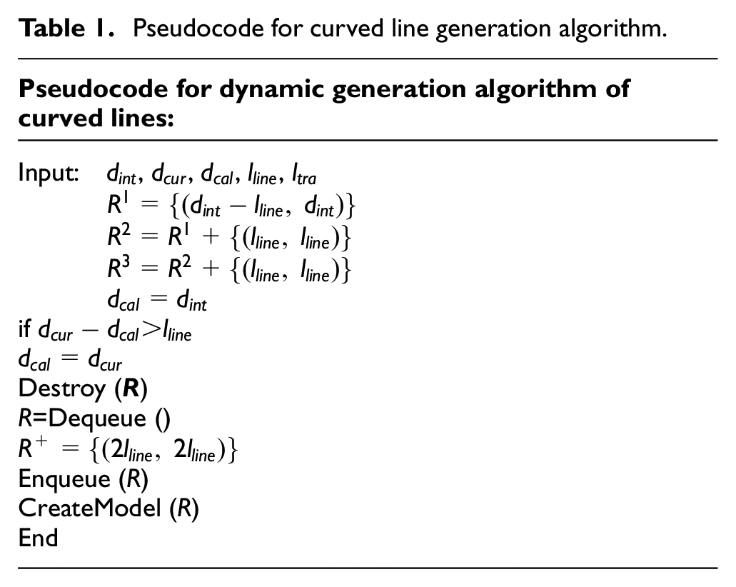
In this paper, the UNITY 3D platform is used to simulate the actual running status of the trains as they pass through curves. Because of computer performance differences, each frame has a different running time that results in different execution times for frames. As a result, Time.deltaTime in UNITY 3D multiplies the previous frame’s running time by the speed, and the result is then used to update the vehicle distance for the next frame to control the vehicle position while the train passes through the curve. It is necessary to implement corresponding algorithms to manage each vehicle and structure to allow a train of eight cars to run efficiently. In this algorithm (see Table 2), the leading train vehicle’s initial position is $d_{\mathrm{int}}$ , the number of vehicles in the train (n) is eight, $l_{\mathrm{veh}}$ represents the length of a single vehicle, $l_{\mathrm{bog}}$ represents the fixed distance between the front and rear bogies of a vehicle, $l_{\mathrm{dis}}$ represents the distance between the ends of adjacent vehicles, $d_i$ represents the position of the ith vehicle, $d_i^f$ represents the position of the front bogie of the ith vehicle, $d_i^b$ represents the position of the rear bogie of the ith vehicle, and the position deviation limit is defined as 0.2 ( $R_{\mathrm{limit}}=0.2$ ). A deviation correction can be applied automatically when the positions of the train and the bogie deviate after setting of the position deviation, i.e., when the deviation exceeds the set deviation limit value when the train is operated on a curve.

Table 2.

Pseudocode for relative position control algorithm for train operation.

Pseudocode for relative position control algorithm of train grouping:
Input:  $d_{\mathrm{int}}$ , $l_{\mathrm{vel}}$ , $l_{\mathrm{bog}}$ , $l_{\mathrm{dis}}$ , $R_{\mathrm{limit}}=0.2$ , n=8
$d_1=d_{\mathrm{int}}-l_{\mathrm{veh}}/2$
For each $d_{i+1},i=[1,n-1]$
$d_{i+1}=d_i-l_{\mathrm{veh}}/2-l_{\mathrm{dis}}$
$d_{i+1}^f=d_{i+1}+l_{\mathrm{bog}}/2$
$d_{i+1}^b=d_{i+1}-l_{\mathrm{bog}}/2$
end for
For each $d_{i+1},i=[1,n-1]$
$L_i=d_{i-1}-d_i$
$\mathrm{\Delta }L=L_i-l_{\mathrm{veh}}-l_{\mathrm{dis}}$
If $\mathrm{\Delta }L>R_{\mathrm{limit}}$
$d_i+=\mathrm{\Delta }L$
If $d_i^f-d_i-l_{\mathrm{bog}}/2>R_{\mathrm{limit}}$
$d_i^f-=d_i^f-d_i-l_{\mathrm{bog}}/2$
If $d_i-d_i^b-l_{\mathrm{bog}}/2>R_{\mathrm{limit}}$
$d_i^b+=d_i-d_i^b-l_{\mathrm{bog}}/2$
end for
End

Twin Data

Data collection

In DT systems, it is essential that the digital representation reflects the real-time status in the physical world accurately, and this necessitates collection of the pertinent information from the real environment.

In this section, we discuss two data acquisition methods: a monitoring-based acquisition system and a measurement and control-based acquisition system. The monitoring-based acquisition system comprises three primary components: a video acquisition unit, a video transmission unit, and a video display unit. During the train’s passage through the curve, multiple cameras act as video acquisition units to enable comprehensive monitoring of the real-time operating status of the train, with the collected image information being converted into data signals. Measurement and control-based acquisition typically involves detection of signals such as voltage, current, pressure, dynamic stress, vibration, noise, temperature, velocity, and displacement signals from the train. Various sensors are used to convert these signals into electrical signals that are then transmitted to the collection equipment for analysis. To display the collected data effectively, relevant data display software can be used to record the different sensor numbers, along with the corresponding acceleration, speed, and other data during the train’s passage through the curve. The data from the different segments can be saved and stored simultaneously to enable easy review and application of specific data collection scenarios in future work. In addition to collection and analysis of multi-source data, the train’s operational status can be monitored by analyzing the vibration acceleration, displacement, and stress characteristics of important elements of the train and the railway transportation equipment. Additionally, the elements of the measurement and control acquisition system include an acquisition unit, a transmission unit, and a display unit. To collect the vibration acceleration, displacement, stress, and triaxial force characteristics, the data acquisition unit uses displacement sensors, acceleration sensors, triaxial force sensors, and attitude sensors. The transmission unit can then transmit data to the corresponding data acquisition system. Finally, the collected data are displayed on the display unit. The attitude sensor must be connected to the computer via a serial port module that converts from Universal Serial Bus (USB) to transistor–transistor logic (TTL). Each frame of data consists of three packets for the acceleration, the angular velocity, and the angle, and each frame is output once every 10 ms at 115,200 baud. Then, based on a specific calculation formula, the corresponding values for the acceleration, velocity, and angle are determined.

The vehicle structure must be equipped with acceleration sensors to monitor its operation; the axle box must be equipped with composite sensors (acceleration) to monitor its bearings and wheelsets. A force measuring wheelset is mounted on the wheelset to monitor the wheel rail force conditions; vibration acceleration sensors are installed on the vehicle to monitor the vehicle’s vibration conditions. By using the sensors associated with these components, comprehensive, and accurate information about the operation and status of the various vehicle components can be captured. The measurement points for the sensor section are described in detail in Table 3.

Table 3.

Partial sensor deployment positions.

Location	Measurement data sensor	Monitored objects
Bogie frame	Accelerometer	Vehicle operating status
Axle box	Composite sensor	Axle box bearings wheelset status
Wheelset	Instrumented wheelset	Wheel rail force
Car body	Vibration acceleration sensor	Vibration state

Data transportation

It is often necessary to design corresponding databases to store and read the required data in real-time and at high speeds. To maintain a secure, reliable, and efficient operating environment, the selection and design of the database are crucial processes. A relational database and a nonrelational database can be included within the database. ³⁵ For driver data transmission to the twin models of the digital world via the network protocols, a nonrelational database called the REDIS server was built, while MYSQL was used to store the train data. The purpose of this design is to improve and maintain the high availability of the relational database by designing a read-write separation mode. Locking is not required for read-only application operations to ensure synchronization. Despite increasing the workload, this mode also accelerates the system’s processing speed. The data security and reliability can be improved by designing nonrelational databases in conjunction with cluster deployment and data modeling. During database design, corresponding entities and attributes are matched for specific data collection times, data types, data numbers, and other characteristics, and the relevant relationships are realized. To associate all data collected under the different test numbers in the different collection test tables, the real-time data table can, for example, be divided using attributes such as test number, speed, acceleration, and time.

In DT systems, real-time mapping is essential, but it places higher demands on the real-time data performance. Although this may not be an issue in theory, in practice, reception of large amounts of data within a short period of time may cause a slow response and delays in data transmission because of the high frequency with which the data pressure acts on the server. This section addresses processing of high-frequency data to reduce the DT delay caused by data collection and the transmission frequency. We use the following methods:

• (1) Segment the data. An interval of 0.5 s is used in the server’s segmented data transmission method. Using a timed function, the server pushes all cached data to the client actively in a multithreaded manner every 0.5 s when the data are transmitted through the User Datagram Protocol (UDP). This approach ensures that the latest collected data are transmitted and prevents packet sticking by clearing the static cache queue. When this method is used, the client will receive data less often, thus resulting in reduced resource consumption.

• (2) Stack the data less frequently. Redundancy in the high-frequency data is caused by high numbers of high-frequency repetitions within a short timeframe. Therefore, every five data cycles, the data are inserted into the data queue. A reduction in the number of data stack presses and optimization of the client’s service response can reduce the performance loss associated with data transmission.

MDF-EKF method

Over time, the estimation state error becomes increasingly large because of an increase in the uncertainty in the test data. To realize the goal of expressing the running state of the train and vehicle on curves accurately in real time, fusion of the multi-sensor data and the model is required to improve the measurement accuracy.

The core algorithm for model-data fusion is centered on the calculation of real-time state corrections that enable autonomous online adjustments to reflect the actual system state in real time. If there is a nonlinear system of train curves when running through curved tracks, it is necessary to establish both the state equation and the measurement equation for the train, and then linearize these equations by taking a first-order approximation that is close to the estimated state of the train. During initialization, the values for the vertical, lateral, and longitudinal vibration displacements, along with the values of the covariance matrix for the initial state estimation errors, are set based on prior knowledge. To continue with the required iteration, three steps must be completed at the end of each iteration. First, the state equation is used in conjunction with the control inputs to predict the current state based on the value of the previous state. Second, the error covariance matrix of the predicted state is calculated; then, the Kalman gain is calculated based on the predicted state, the measurement matrix, the measurement noise covariance, and additional parameters. A more accurate state estimation value is then obtained by combining the measured values with the Kalman gain and subsequently updating the state estimation error covariance matrix. Finally, a data model update converts the uncertain data into information about the train’s running behavior based on real-time data. With continuous iterations, we can visualize the actual state of the train when running through curved tracks in real time.

The MDF-EKF method used in this section is an online optimal estimation algorithm that enhances the traditional Kalman filter to enable better handling of nonlinear systems. This algorithm fully uses the data collected during the testing processes, applies recursive techniques to eliminate any random noise, and determines the spatial state values online accurately. ³⁶ Based on an analysis of the dynamic model of a train passing through a curve, its state equation and its measurement equation can be constructed, ³⁷ as shown in equations (1) to (4).

$$\begin{array}{c}\stackrel{·}{l}(t)=f(\mathit{l}(t),\mathit{u}(t),\mathit{w}(t))\hfill \\ \multicolumn{1}{c}{\mathit{c}(t)=h(\mathit{l}(t),\mathit{v}(t))}\end{array},$$

(1)

The state variables are:

$$\mathit{l}\left(t\right)=[x,y,z,\varphi ,\beta ,\psi ],$$

(2)

The measurement output is:

$$\mathit{c}\left(t\right)=[x\prime ,y\prime ,z\prime ,\varphi \prime ,\beta \prime ,\psi \prime ],$$

(3)

The control variables are:

$$\mathit{u}\left(t\right)=[a_x,a_y,a_z],$$

(4)

where $f$ represents the state function; $h$ represents the measurement function; $a_x,a_y,a_z$ represent the longitudinal, transverse, and vertical accelerations of the vehicle, respectively; $\mathit{w}(t)$ and $\mathit{v}(t)$ represent the independent process noise and the observation noise, respectively, and their corresponding covariance matrices are represented by Q and R, respectively.

By combining the vehicle dynamics equations, the state matrix, the control matrix, and the measurement matrix can be obtained. The state matrix $F\left(t\right)$ and the measurement matrix $H^{*}$ can be replaced with the Jacobian matrix. When the state matrix variable is n, the Jacobian matrix solution process can then be expressed as: ²⁹

$$F\left(t\right)=\frac{\partial f}{\partial l}=\left[\begin{array}{ccc}\frac{\partial f_1}{\partial l_1}\hfill & \cdots \hfill & \frac{\partial f_1}{\partial l_n}\hfill \\ \multicolumn{1}{c}{⋮}& \ddots \hfill & ⋮\hfill \\ \multicolumn{1}{c}{\frac{\partial f_n}{\partial l_1}}& \cdots \hfill & \frac{\partial f_n}{\partial l_n}\hfill \end{array}\right],$$

(5)

$$H^{*}=\frac{\partial h}{\partial l}=\left[\begin{array}{ccc}\frac{\partial h_1}{\partial l_1}\hfill & \cdots \hfill & \frac{\partial h_1}{\partial l_n}\hfill \\ \multicolumn{1}{c}{⋮}& \ddots \hfill & ⋮\hfill \\ \multicolumn{1}{c}{\frac{\partial h_n}{\partial l_1}}& \cdots \hfill & \frac{\partial h_n}{\partial l_n}\hfill \end{array}\right],$$

(6)

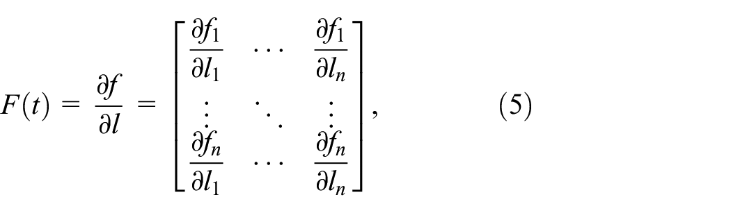
By assuming a time interval of ãt, the linearized state transition matrix A * can be expressed as:

$${\mathit{A}}^{*}\left(\mathit{t}\right)={\mathit{e}}^{\mathit{F}\left(\mathit{t}\right)\mathrm{\Delta }\mathit{t}}\approx \mathit{I}+\mathit{F}(\mathit{t})\mathrm{\Delta }\mathit{t},$$

(7)

Then, only N−1 measurement values at the current time and previous times are selected for the optimal estimation calculation. Based on this approach, the discrete state equation and the measurement equation are obtained as follows: ²⁹

$$L_k=A_{k|k-1}{L}_{k-1}+B_{k|k-1}{U}_{k-1}+W_{k-1},$$

(8)

$$C_k=H_k{L}_k+V_k,$$

(9)

where $L_k$ and $L_{k-1}$ represent the state matrices at a time $k$ and a time $k-1$ , respectively; $U_{k-1}$ represents the control variable matrix at time $k-1$ ; $A_{k|k-1}$ represents the state transition matrix for prediction of time k at time k−1; $B_{k|k-1}$ represents the measurement transition matrix for prediction of time k at time k−1; $H_k$ represents the measurement matrix at time k; $W_{k-1}$ represents the process noise matrix at time k−1; and $V_k$ represents the measurement noise matrix at time k.

The specific process of autonomous correction in model-data fusion research (see Figure 2; the corresponding pseudocode is shown in Table 4) can be divided into the following steps:

• (1) Set the storage of the initial value $L_{k-1}^{*}$ and the initial covariance matrix $P_{k-1}^{*}$ ;

• (2) Predict the state equation: ${\overline{L}}_k=A_{k|k-1}{L}_{k-1}^{*}$ ;

• (3) Linearize the state transition matrix and the measurement matrix: $\mathit{A}\to \mathit{A}*,\mathit{H}\to \mathit{H}*$ ;

• (4) Predict the covariance: $P_{k|k-1}^{*}=A_{k|k-1}^{*}{P}_{k-1}^{*}{A}_{k|k-1}^{*T}+Q_{k-1}$ ;

• (5) Predict the measurement matrix: ${\overline{C}}_k=H_k{\overline{L}}_k$ ;

• (6) Obtain the measurement error: $R_k=C_k-{\overline{C}}_k$

• (7) If $k<<N,{\hat{R}}_k^{*}=R$ ;

  if $k>N,{\hat{R}}_k^{*}=\sum _{i=k-N+1}^k\frac{1-\epsilon }{1-{\epsilon }^N}{\epsilon }^{k-i}·[(r_i-{\hat{r}}_k^{*}){(r_i-{\hat{r}}_k^{*})}^T-\frac{N-1}{N}{H}_k^{*}{P}_{k|k-1}^{*}{H_k^{*}}^T]$ , where $\epsilon$ represents the weighting coefficient, which has an interval range of 0.95 to 0.995.

• (8) Obtain the filtering gain: $K_k^{*}=P_{k|k-1}^{*}{H}_k^{*T}(H_k^{*}{P}_{k|k-1}^{*}{H}_k^{*T}+{\hat{R}}_k^{*}{)}^{-1}$

• (9) Update the status: ${\hat{L}}_k^{*}={\overline{L}}_k+K_k^{*}(Z_k-H_k^{*}T{\overline{L}}_k)$

• (10) Update the covariance: $P_k^{*}=(I-K_k^{*}{H}_k^{*})P_{k|k-1}^{*}{(I-K_k^{*}{H}_k^{*})}^T+K_k^{*}{\hat{R}}_k^{*}{K}_k^{*}T$ . According to the literature, ³⁶ simplifying and updating the covariance can then give: $P_k^{*}=(I-K_k^{*}{H}_k^{*})P_{k|k-1}^{*}$ .

Figure 2.

Update calibration process.

Table 4.

Pseudocode for the MDF-EKF method.

Pseudocode for the MDF-EKF method
Input:  $L_0^{*}$ , $P_0^{*}$ , $Q_0$ , $\mathit{A}*$ , $\mathit{H}*$ Initial  $P_0^{*}$ and $L_0^{*}=$ [ $x_0$ , $y_0$ , $z_0$ , ${\varphi }_0$ , ${\beta }_0$ , ${\psi }_0$ ]
For each $\mathrm{k}=[1,N]$
$L_k^{*}=\mathit{A}*L_{k-1}^{*}$ ;
$P_k^{*}=\mathit{A}*P_{k-1}^{*}\mathit{A}*\prime +Q_{k-1}$ ;
${\mathrm{y}}_k=\mathit{H}*L_k^{*}$ ;   $K_k^{*}=P_k^{*}\mathit{HH}\prime *\mathrm{inv}(\mathit{H}*P_k^{*}\mathit{H}*\prime +R_k)$ ;   $L_k^{*}=L_k^{*}+K_k^{*}({\mathrm{z}}_k-{\mathrm{y}}_k)$ ;   $P_k^{*}=(\mathrm{I}{K}_k^{*}\mathit{H}*)P_k^{*}$ ;
end for
End

A DT system is not complete without a model of the relevant physical entities, which includes the ability to reflect the operating status of these entities in real-time, i.e., to follow their changes in the real world. A single request approach is used in data-driven modeling to avoid unnecessary resource consumption being caused by multiple requests and thus enable the virtual model to receive the real-time data from the server. As soon as the server receives an access request, it queries the databases sequentially through a Bloom filter. Upon receiving real-time data in the client, the virtual model desterilizes the received data to obtain information that describes the operational status of the relevant physical entity. The data are then filtered at fixed time intervals, which are consistent with the Fixed Update interval, to prevent rendering delays being caused by an influx of data within a short period. Subsequently, the virtual model’s states are updated at these fixed time intervals in alignment with the Fixed Update timing. This method ensures that even if abnormal data are received, the digital model states are updated to reflect the real-time states of the physical entity and thus effective data-driven modeling is achieved. Ultimately, model visualization requires real-time model updates, which means that when the virtual model does not receive any information, it remains in its initial state; the speed, time, and other information are then updated in real time when the model receives the relevant dynamic information. As a result, the model can reflect the motion status at different times and in real time. A diagram showing the processes involved in the MDF-EKF method can be found in Figure 3.

Figure 3.

MDF-EKF method diagram.

Case study

Establishment of twin models

The twin model transmits vital information, including performance, structural, geometry, and assembly information, while the train passes through curved tracks. Through polygonal modeling, the specific features of the vehicle system are described in detail using Autodesk Maya 2018 software (Autodesk, Inc., San Francisco, CA, USA). This creates a more realistic representation of the vehicle’s complex structure. Real-time three-dimensional graphic data are calculated and output to obtain an accurate model of the train when passing over curved tracks. In this work, we developed a simplified train virtual model based on the parameters and the structure of the CRH380B high-speed train. Additionally, a model of the entire train formation was created to analyze the behavior of this train when negotiating curves. According to the literature, ³⁸ the maximum axle load of the CRH380B high-speed train is 17 t, and its traction power is 8800 kW. The specific basic parameters for this vehicle are listed in Table 5.

Table 5.

Vehicle parameters of CRH380B high-speed train.

Parameters	Units	Value
Center distance of bogie	mm	17,375
Wheelbase	mm	2500
Wheel rolling circle lateral span	mm	1493
Wheel rolling circle diameter	mm	920
Inner distance of wheelset	mm	1353
Wheel profile		S1002CN
Length	mm	24,825
Width	mm	3257
Height from rail surface	mm	3915
Height between the floor and the rail surface	mm	1260

These terms describe the various dimensions and characteristics related to the bogie, the wheels, and overall configuration of a rail vehicle, including the distance between the bogie centers, the wheelbase, the lateral span and the diameter of the wheel rolling circles, the inner distance of the wheelset, and the wheel profile, along with the length, width, height from the rail surface, and height between the floor and the rail surface of the vehicle.

The bogie features an H-shaped welded frame with a wheel diameter of 920 mm and rotary arm-type axle box positioning. The primary suspension system uses spiral springs and vertical shock absorbers, while the secondary suspension system uses air springs with auxiliary rubber piles to support the vehicle body directly. Anti-roll bars are connected in parallel on each side of the bogie, and a Z-shaped traction rod device is used. An anti-roll torsion bar device is also installed to create a simplified bogie model, as illustrated in Figure 4(a). Additionally, a three-dimensional vehicle model of the CRH380B high-speed train is constructed using these parameters. The vehicle model includes the body, the frame, the wheelset, and two series of suspension systems, resulting in a simplified vehicle model. Given that the CRH380B high-speed train uses an eight-car configuration with four motor cars and four trailers, a simplified train model is established by incorporating a coupler buffer device, as illustrated in Figure 4(b).

Figure 4.

Virtual models. (a) Bogie model; (b) train model.

Next, we reconstruct the terrain and the curved route based on the selected curve route. The terrain construction process involves three main steps: selection of the reconstruction area, extraction of the dataset, and reconstruction of the terrain. During the reconstruction region selection stage, which is based on the spherical Mercator projection,^39,40 the focus of the process is on calculation of the center point of the reconstruction region, converting this point into the origin of the world coordinates, and then mapping the selected pixel coordinate domain onto the World Geodetic System WGS-84 latitude and longitude coordinates used in this paper. During the dataset extraction stage, the texture data from the selected terrain area and the terrain elevation data are obtained separately. Finally, during the terrain reconstruction stage, the segmented terrain is arranged based on the longitude and latitude coordinate values to form the complete terrain, and textures are then added.

The line from Chaoyang Station to Beipiao Station on the Beijing-Shenyang high-speed railway line was selected as the research line for this study. An area of 54.8 × 36.54 km² between Chaoyang City and Beipiao City was reconstructed, with its center point at a longitude of 120.257° and a latitude of 41.519°. The elevation map and the texture data from the selected area were organized to reconstruct the terrain and render its overall effect. The reconstructed three-dimensional terrain can display the undulations in the terrain and features such as rivers, forests, and mountains realistically. The rendered terrain map is shown in Figure 5. Based on the established terrain, a track curve model was then created to generate the curved lines.

Figure 5.

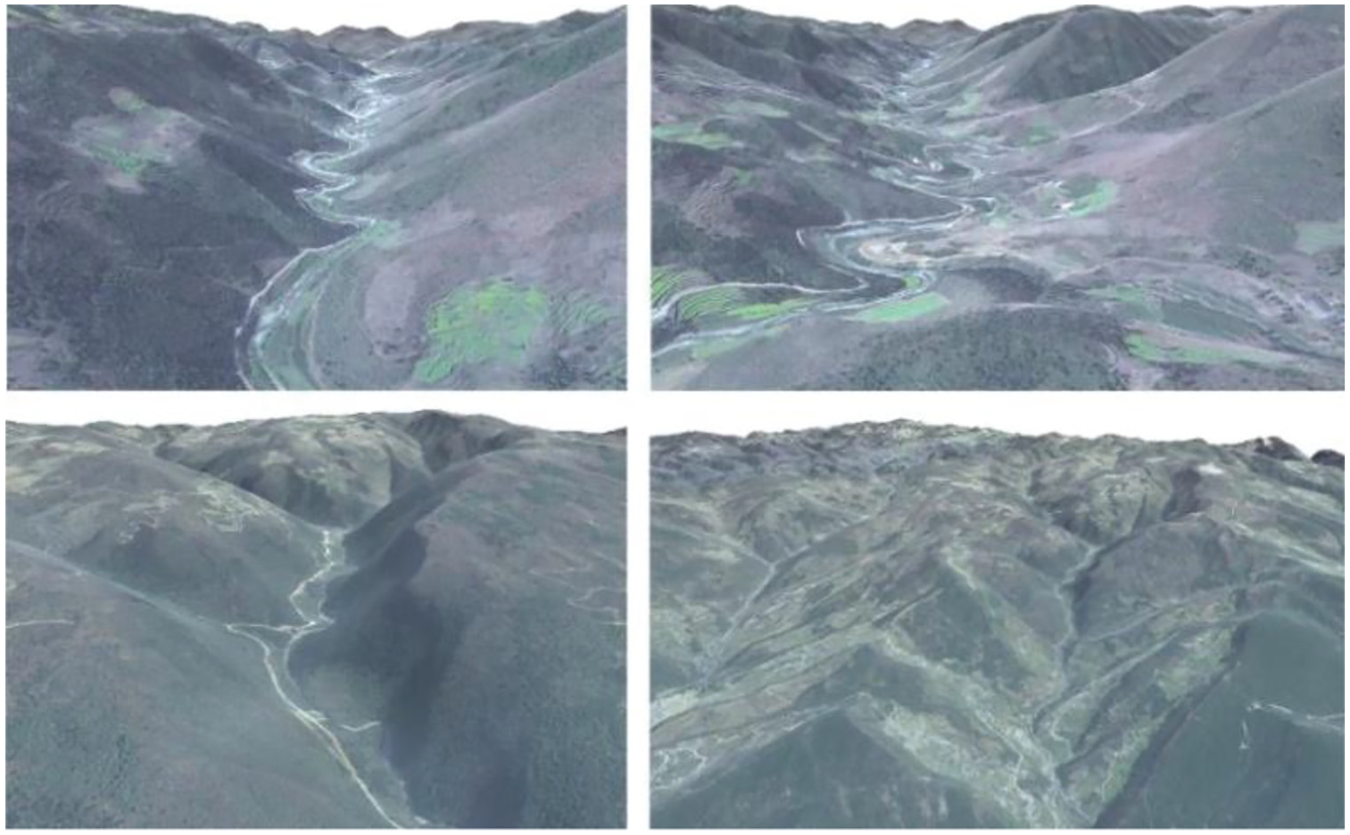
Terrain reconstruction images.

Using the conventional structural parameters of railway lines, basic models of elements such as steel rails, sleepers, fasteners, and track beds were constructed to form a basic model library. The characteristics of tunnels, elevated lines, and other track structures, along with basic parameters such as the distribution spacing, were then analyzed based on the line information. The positional relationships between the line, the model, and the terrain were calculated using coordinate transformation principles. Finally, different curve routes were constructed based on the identified location information. The total distance from Chaoyang Station to Beipiao Station is approximately 37 km and features complex terrain with bridges and tunnels. The line model constructed here includes structures such as steel rails, sleepers, bridge piers, pillars, contact lines, and tunnels.

Twin data analysis

Using DTs, train curve passage safety can be enhanced by analyzing the twin data while focusing on the safety of train curve passages. Several twin data types exist, including structural data, operational data, and indicator data, which could enable implementation of a real-time driving twin model. Table 6 lists the available primary twin data.

Table 6.

Partial twin data description.

Data Name	Unit	Data Description
Measured speed	km/hour	Operational data
Vertical force of outer rail	kN	Operational data
Lateral force of outer rail	kN	Operational data
Vertical force of inner rail	kN	Operational data
Lateral force of inner rail	kN	Operational data
Lateral displacement of inner rail	mm	Operational data
Lateral displacement of outer rail	mm	Operational data
Vertical displacement of outer rail	mm	Operational data
Vertical displacement of external sleeper	mm	Operational data
Lateral displacement of external sleeper	mm	Operational data
External sleeper acceleration	g	Operational data
External rail acceleration	g	Operational data
Internal rail acceleration	g	Operational data
Wheel load reduction rate	—	Operational data
Internal rail derailment coefficient	—	Indicator data
Derailment coefficient of outer track	—	Indicator data
Curve superelevation	mm	Structural data
Curve radius	mm	Structural data
Curve length	mm	Structural data

There are several types of twin data, with each having its own meaning.

• (1) Structural data: This data type encompasses the physical information of the vehicle curve model, including parameters such as the vehicle model, the curve radius, the curve length, and the superelevation. These data not only affect the external structure of the twin 3D model but also can be adjusted according to various needs and specific services.

• (2) Operational data: This data type refers to data that reflect the operational status of the model, including the operating speed, the axle box acceleration, the vertical wheel-rail force, the lateral wheel-rail force, the vertical displacement, and the lateral displacement. These data can indicate real-time changes in vibration, performance, and other states as the train navigates curves in the DT model.

• (3) Indicator data: This data type consists of safety indicators during train curve passage, including the derailment coefficient, the lateral wheel-rail force, and the wheel load reduction rate. These indicators are typically derived from historical operational data and provide critical support for predictive and preventive measures in DTs.

The data collection frequency is 20 Hz. The collected data are cached in the memory, and collections of 1000 data points are batch-inserted into the database using SqlSessionFactory. Experimental verification performed on a Windows 10 system platform with eight cores and 16 threads showed that it takes only 1 to 2 s to insert 1000 data points. Real-time data are then transmitted via network protocols. Upon receiving the data, the server then performs the relevant processing and desterilizes the serialized data to extract the various data. The received state data are subsequently used to drive operation of the DT model.

To achieve interoperability between the data and the models, three protocols are used in this section: Hypertext Transfer Protocol (HTTP), ⁴¹ UDP, ⁴² and WebSocket. ⁴³ These protocols enable real-time data transmission and communication. These protocols are used in this section as part of the DT data transmission system. After the Netty server receives the real-time collected data, these protocols are applied to enable real-time reception of client data, thus providing strong support for driving real-time operation of the DT model. Given that traditional TCP protocols can only send requests in one direction at a time, leading to low transmission efficiency, this section uses the HTTP, UDP, and WebSocket protocols comprehensively. These three network protocols enable data transmission and interconnection between data acquisition devices, data servers, and UNITY 3D clients. HTTP is used for the data transmission between the UNITY 3D client and the server, WebSocket pushes the real-time collected data, and UDP sends data from the data acquisition devices to the servers for storage. This multi-protocol data transmission process is illustrated in Figure 6.

Figure 6.

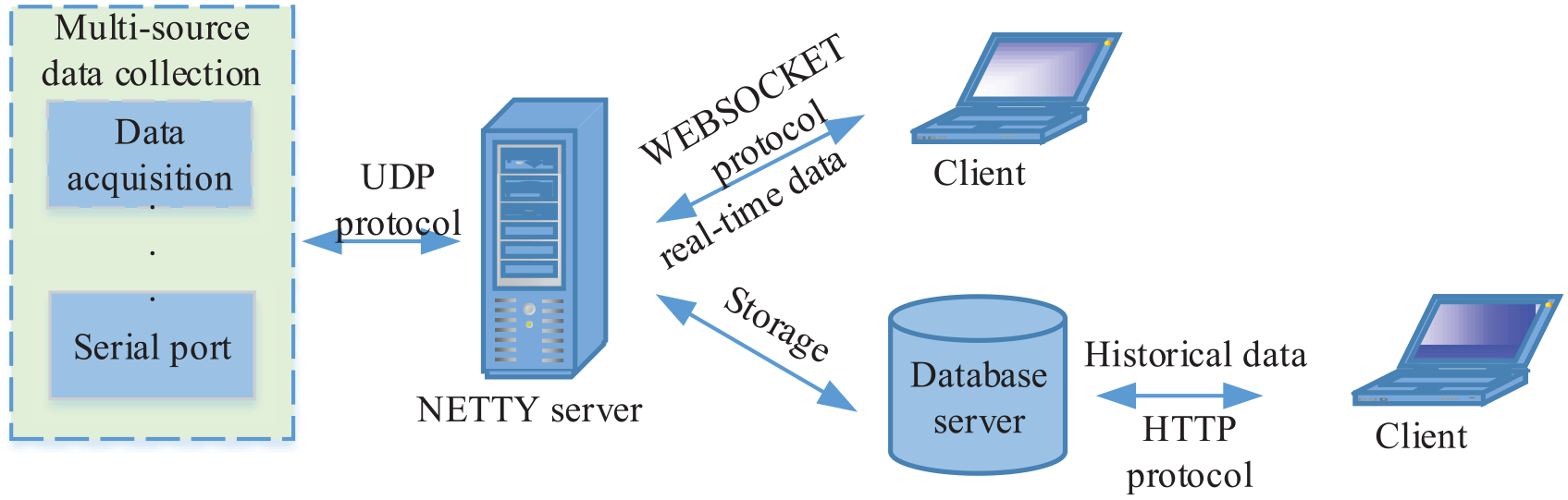
Multi-protocol data transmission process.

As illustrated in Figure 6, the data transmission process includes two main parts: transmission of the real-time collected data and transmission of historical data. For real-time data collection during transmission tests, the main steps are described as follows: (1) Send the data collected by the data acquisition device to the Netty server using the UDP protocol. (2) Actively push the UDP-collected data to the client using the WebSocket protocol. (3) On receiving the data, the client performs deserialization and then visualizes the real-time data changes. For transmission of historically collected data, the main steps are: (1) Send the data collected by the data acquisition device to the Netty server using the UDP protocol. (2) Actively push the UDP-collected data to the database server using the WebSocket protocol. (3) Establish a connection between the client and the data server, and then send a request. (4) Using the HTTP protocol, the server transmits the data to the client. (5) On receiving the data, the client desterilizes it to acquire data that describe the running status of the model and then displays the real-time data changes.

Experimental results

Using the example of a train traveling on the Beijing–Shenyang high-speed railway, the model-data fusion analysis procedure is demonstrated in this work. The CRH380B high-speed train is used as the experimental object in this paper. The line from Chaoyang to Beipiao Station, which is 60 km long, with six curves and 24 longitudinal slope sections, was selected as the main research section to meet the requirements for diversity of data collection. Table 7 provides information about the six curve sections. The train passes through these curves at 250 km/hour and 350 km/hour, and collects experimental data at intervals of 0.01 s, which is consistent with the FixedUpdate time interval used in UNITY 3D. In this paper, model-data fusion methods are used to estimate the train’s state variables (i.e., the longitudinal displacement (X), the lateral displacement (Y), the vertical displacement (Z), the roll angle (ϕ), the nodding angle (β), and the shaking angle (ε)) at various times and positions.

Table 7.

Characteristics along the curve route.

	Curve radius R (m)	Front transition curve length l (m)	Rear transition curve length l (m)	Curve length L (m)	Intermediate straight line length (m)	Actual superelevation (mm)
1	9000	530	530	4451.607	—	120
2	12,000	370	370	1363.027	4462.098	90
3	10,000	470	470	1320.557	4208.416	110
4	8000	590	590	1671.202	22,862.502	125
5	8000	590	590	3048.247	4374.444	125
6	10,000	470	470	1318.280	3881.959	100

Model-data fusion methods were used to estimate the train’s state variables by applying extended Kalman filtering (MDF-EKF), Kalman filtering (KF), and unscented Kalman filtering (UKF). These estimated results were then compared with the test results, as shown in Figure 7.

Figure 7.

Comparison of estimated and tested values for three model-data fusion methods.

From Figure 7, it is evident that although all three fusion methods exhibited good tracking performances, the estimated states are close to the real states across most time periods. The KF method showed significant errors in the longitudinal displacement, the lateral displacement, and the vertical displacement. The UKF method presented significant errors in estimation of the roll angle, the nodding angle, and the shaking angle. The MDF-EKF method proposed in this study exhibited minimal deviations in the longitudinal displacement, the lateral displacement, the vertical displacement, the roll angle, the nodding angle, and the shaking angle throughout the entire process. To provide a further illustration of the accuracy of MDF-EKF when estimating the system state, its deviation from the predicted values is explained using absolute deviations. The bias estimates for the different filtering algorithms are presented in Figures 8 to 10.

Figure 8.

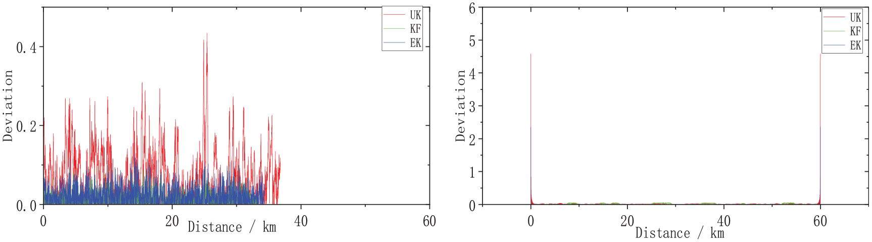
Deviation distribution maps of the longitudinal displacement and the lateral displacement.

Figure 9.

Deviation distribution maps of the vertical displacement and the roll angle.

Figure 10.

Deviation distribution maps of the nodding angle and the shaking angle.

In Figure 8, the KF method shows significant errors in both the longitudinal displacement and the lateral displacement, with maximum errors of 2.85 and 1.46, respectively. The MDF-EKF method proposed in this study exhibits minimal deviations in the longitudinal displacement and the lateral displacement throughout the entire process, with maximum deviations of 0.7 and 0.8, respectively. The overall deviation from the application scenario has a value of less than 3, which is considered acceptable.

In Figure 9, the KF method shows significant errors in the vertical displacement, with a maximum error of 2.69. The UKF method displays significant errors in estimation of the roll angle, with a maximum error of 0.58. The MDF-EKF method proposed in this study shows minimal deviations in the vertical displacement and the roll angle throughout the entire process, with maximum deviations of 2.45 and 0.31, respectively. The overall deviation from the application scenario again has a value of less than 3, which is considered acceptable.

In Figure 10, the UKF method displays significant errors in estimation of both the nodding angle and the shaking angle, with maximum errors of 0.43 and 0.45, respectively. The MDF-EKF method proposed in this study shows minimal deviations in the nodding angle and the shaking angle throughout the entire process, with maximum deviations of 0.30 and 0.08, respectively. The overall deviation from the application scenario has a value of less than 0.5, which is again considered acceptable.

Overall, the KF method shows significant errors in the longitudinal displacement, the lateral displacement, and the vertical displacement, with maximum errors of 2.85, 1.46, and 2.69, respectively. The UKF method shows significant errors in estimation of the roll angle, the nodding angle, and the shaking angle, with maximum errors of 0.58, 0.43, and 0.45, respectively. The proposed MDF-EKF method exhibits minimal deviations in the longitudinal displacement, the lateral displacement, the vertical displacement, the roll angle, the nodding angle, and the shaking angle throughout the entire process, with maximum deviations of 0.7, 0.8, 2.45, 0.31, 0.30, and 0.08, respectively. The overall deviation from the application scenario has a value of less than 3, which is considered acceptable. These comparison results indicate that the MDF-EKF method offers superior performance when compared with the other fusion methods in terms of its ability to estimate and describe the state of the vehicle accurately during the train curve-passing process.

Additionally, we analyzed the running speed characteristics of trains when traveling at 250 km/hour and 350 km/hour to verify the feasibility of the proposed method, and we compared the MDF-EKF method with the particle filtering (PF) algorithm (where 1000 particles are used and a 100 iterations are performed) for estimation of the state variables of the train at different positions and times (including the longitudinal displacement, the lateral displacement, the vertical displacement, the roll angles, the nodding angle, and the shaking angle). The MDF-EKF and PF methods were compared at 250 km/hour in terms of the longitudinal displacement (X), the lateral displacement (Y), and the vertical displacement (Z), with results as shown in Figure 11. In Figure 12, the results for estimation of the rolling angle (ϕ), the nodding angle (β), and the shaking angle (ε) obtained using the two fusion methods are shown.

Figure 11.

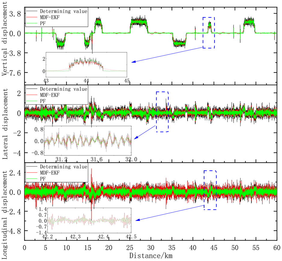
Results of comparison of the MDF-EKF and particle filtering (PF) methods at 250 km/hour.

Figure 12.

Results of comparison of the MDF-EKF and PF methods at 250 km/hour.

The MDF-EKF and PF methods were then compared at 350 km/hour in terms of the longitudinal displacement (X), the lateral displacement (Y), and the vertical displacement (Z), with results as shown in Figure 13. In Figure 14, the results for estimation of the rolling angle (ϕ), the nodding angle (β), and the shaking angle (ε) obtained using the two fusion methods are shown.

Figure 13.

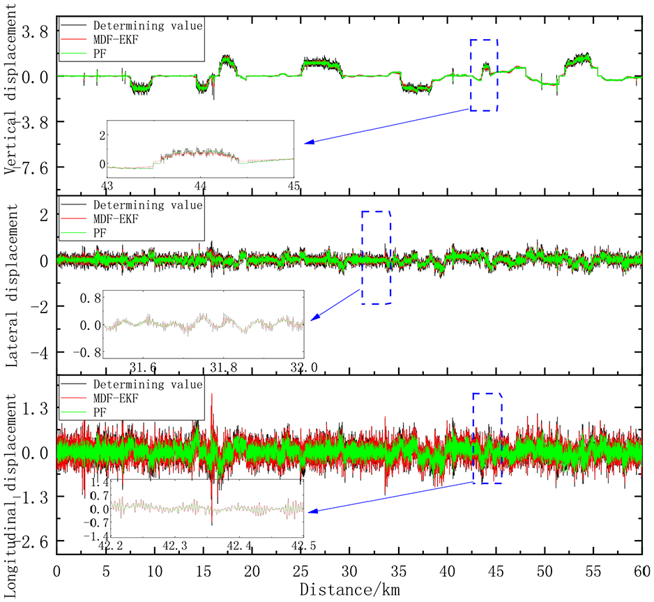
Results of comparison of the MDF-EKF and PF methods at 350 km/hour.

Figure 14.

Results of comparison of the MDF-EKF and PF methods at 350 km/hour.

In Figure 11, the deviations between the measured values and those estimated using the MDF-EKF method and the PF algorithm are shown for three displacements: the vertical displacement, the lateral displacement, and the longitudinal displacement. It is noticeable that the values estimated by the MDF-EKF and PF deviate significantly from the measured values at around 43 to 45 km, with both estimated values being significantly higher than the measured values. The MDF-EKF and PF values also deviated from the measured values in terms of the lateral displacement at around 31 to 33.0 km. The value estimated using the PF approach fluctuates greatly within this range and is higher than the measured value, and although the value estimated using the MDF-EKF method fluctuates similarly, the amplitude of these fluctuations is relatively small. Within the test section, it was found that there were significant deviations between the MDF-EKF and PF values, and the PF fluctuations are most evident during these intervals.

In Figure 12, we show the deviations between the measured values and the estimated MDF-EKF and PF values for three angles: the shaking angle, the nodding angle, and the roll angle. In the range from 0 to 10 km, there is a relatively small deviation between the MDF-EKF and PF estimates and the measured values of the shaking angle. However, between 10 and 12 km, this deviation increases, before then decreasing after 12 km, although the deviation remains positive. There are also small deviations over the range from 0 to 28 km for the nodding angle, and this is followed by a large positive deviation in the PF values and a small positive deviation in the MDF-EKF value from 28–30 km. As the PF deviation decreases after 30 km, and when the MDF-EKF deviation decreases, it then stabilizes. For the roll angle, there are small deviations over the range from 0 to 28 km, followed by a significant positive deviation in the PF value and a small positive deviation in the MDF-EKF value over the 28- to 30-km range. Beyond 30 km, the PF deviation decreases rapidly and then stabilizes with a negative deviation, and the MDF-EKF deviation decreases as a result. In general, the MDF-EKF and PF deviations are both relatively small, but significant deviations are observed within specific intervals, particularly in areas with dramatic angle changes.

In Figure 13, measured displacements and those from the MDF-EKF and PF methods are compared for the vertical displacement, the lateral displacement, and the longitudinal displacement. At around 43 to 45 km, there is a significant deviation between the measured values and those of the MDF-EKF and PF methods, with their estimated values being considerably higher than the measured results. The estimated longitudinal displacement values differ significantly from the measured value at around 42.2 to 43.5 km. The MDF-EKF method has a relatively small fluctuation amplitude when compared with that of the PF method and fluctuates greatly. The PF estimate fluctuates much more than the measured values, and the MDF-EKF value fluctuates much more than the measured values. It is important to note that there are significant differences between the measured values and the MDF-EKF and PF values within specific distance ranges. The PF fluctuations are often more pronounced than the MDF-EKF fluctuations.

As shown in Figure 14, the deviations between the measured values and the MDF-EKF and PF values are assessed based on three angles: the shaking angle, the nodding angle, and the roll angle. Between 0 and 10 km, the deviation between the MDF-EKF and PF estimates and the measured values is small, but over the range from 10 to 12 km, there is a significant positive deviation. Over distances from 12 to 28 km, the deviations for the PF and MDF-EKF methods are minimal, with a larger positive deviation being observed for the PF from 28 to 30 km, and a minimal deviation being observed for the MDF-EKF beyond 30 km. A significant positive deviation in the PF value and a small positive deviation in the MDF-EKF value can be observed from 28 to 30 km. Within the 30 km range, the PF deviation decreases rapidly and then stabilizes after a negative deviation appears, while the MDF-EKF deviation decreases correspondingly. Generally, there is slight deviation between the MDF-EKF and PF estimates, but there may be significant deviations when the angle changes are dramatic.

In Figure 15, the two fusion methods (MDF-EKF and PF) are compared under six operating conditions (longitudinal, lateral, and vertical displacements, and rolling, nodding, and shaking angles) at different speeds (250 km/hour and 350 km/hour). The different fusion methods show significant differences between their deviation values at the different speeds under different working conditions; although the deviation values estimated at 350 km/hour tend to be higher than those estimated at 250 km/hour, these deviations both stay within 3.5, thus indicating that both methods are accurate. Calculations performed using the PF algorithm at 350 km/hour or 250 km/hour are generally slower than those performed using the MDF-EKF method at those speeds.

Figure 15.

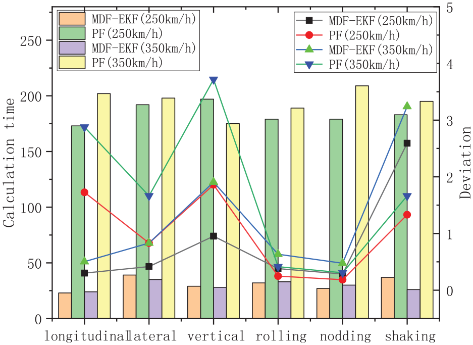
Comparison of the two fusion methods.

By combining our estimates with measurement data gathered during train passage through a curve, the MDF-EKF and PF methods were able to determine suitable estimated values. It is true that both the PF and MDF-EKF methods are capable of capturing train operation accurately. However, the PF requires significant computing resources and real-time performance is difficult to guarantee, thus limiting its application to DTs for real-time scenarios. As a result of using MDF-EKF, the twin models can be driven in real time to reflect the true state of the train during the curve passing process, thus providing a basis for further prediction of future states and provision of dual services such as decision optimization and adjustment.

Discussion

Discussion

The achievement of “fully digital twin trains” remains a distant goal, and the route is marked by numerous unforeseeable challenges in terms of vehicle system dynamics and related disciplines. In the context of railway vehicle dynamics models for DTs, the primary disparities between DT track vehicle dynamics models and the traditional models revolve around the way in which two key issues are addressed. The first is the necessity of model accuracy as a fundamental condition for creation of DTs. In many instances, computational limitations make it challenging to implement exceptionally precise models because of resource constraints, model complexity, and other factors. The second issue involves ensuring the real-time performance of these models.

In the development of a DT-oriented model, it is imperative to integrate the data into traditional railway vehicle dynamics models. One practical approach involves amalgamating the test data with physical models to create a fusion model that simulates the specific behavior of a single train accurately while also capturing the distinctions and variations between trains of the same type. This step will be pivotal in the development of DT trains. Because the Kalman filter is constructed based on a Gaussian assumption, its performance will decrease significantly when faced with non-Gaussian noise. ⁴⁴ Furthermore, in scenarios involving highly nonlinear systems, e.g., railways, Kalman filters can cause significant linearization errors that lead to inaccurate state estimation and reduced filter stability. When it comes to non-Gaussian noise and highly nonlinear system dynamics, PF offers some advantages. The model can adapt to complex system characteristics by continuously resampling and updating the particle weights, and therefore it tracks the state changes accurately. DTs, however, have a relatively large state space dimension, which means that PF requires large amounts of computing resources. As a result, it is difficult to guarantee real-time performance and thus the application of DTs in real-time scenarios is limited. By taking both the nonlinear characteristics of railway systems and the real-time requirements of DTs into account, the MDF-EKF method can address the real-time requirements of DTs comprehensively. By optimizing the calculations of nonlinear systems based on their state equations, the method reduces linearization errors, improves the state estimation accuracy, and ensures real-time calculations are possible for nonlinear systems.

Future Studies

As the digital infrastructure of the railway system evolves, further development and use of vehicle dynamics will be essential to test the models and the various data collection and fusion technologies for DT trains and their components. A comprehensive digital model of a train will simulate its performance, behavior, and interactions in various scenarios. The process of creating DT trains can be divided into two parts: the first part involves establishing a universal model of the train, which is usually based on physics, and the second part focuses on creation of personalized models by integrating specific data into the universal model. Additionally, each DT train will update continuously with real-time data to ensure that it provides an accurate and current representation of the physical train.

From the initial design phase through the development and operation and maintenance phases, the framework ensures synchronous reflection of the states of physical trains. This process not only enhances the fidelity of DTs but also enables stakeholders to conduct comprehensive multi-source data and predictive analyses. Using advanced data fusion technology, the platform serves as a foundation throughout the entire lifecycle of the train that can adapt to the constantly evolving needs of physical systems to ensure their safe and efficient operation. However, the accuracy and reliability of DT trains largely depend on the precision and the comprehensive nature of their vehicle system dynamics models. Clear vehicle system dynamics models will enable DTs to simulate real-world scenarios, predict potential problems, and then propose feasible solutions.

Deep learning can make use of the large amounts of historical and real-time data in DT systems, enabling them to learn the complex characteristics of the system more accurately as the data volumes increase. It is expected that nonlinear relationships and non-Gaussian noise processing will also be developed further. Consequently, combining deep learning with other model fusion methods may represent the next research step. In addition to using deep learning’s advantages in complex systems and noise processing, Kalman filters also use the recursive mechanism to solve state estimation problems in practical applications, thus making these filters more effective.

Conclusions

In this paper, we propose a model-data fusion method for a train passing through a curved track toward development of DTs. A three-dimensional virtual model that reflects the real scene of the train’s curve passage is established and visualized, and the MDF-EKF method is then applied to obtain the operating state variables of the trains and vehicles accurately, thus reducing the state description errors caused by system uncertainty. Specifically, based on the curved line information from the Beijing–Shenyang high-speed railway, a corresponding curved line physical model was developed and a physical model of a CRH380B high-speed train was established. Additionally, by applying an automatic generation algorithm for the curved lines and a control algorithm for the positioning of grouped trains, real-time control of the grouped trains’ positions during the curve passage was achieved. It is possible for the MDF-EKF method to provide state estimation results in real-time system scenarios without processing large numbers of random particles like the PF technique, thus saving considerable computation time and resources, and making it better able to perform real-time processing in systems with strong real-time requirements. Additionally, throughout the entire process of the train passing through the curved track, the MDF-EKF method shows the smallest deviations when compared with other fusion methods. Deep learning could be combined with other fusion methods in future work to enable twin services, e.g., state prediction, that ensure safe and efficient system operation.