
Abstract
To improve the stability of the maglev train’s levitation and enhance its dynamic performance during high-speed operation, this paper establishes a control strategy based on backstepping control theory and fuzzy neural network. Firstly, this paper presents a vehicle/guideway numerical model based on the Shanghai Maglev line (SML) structure, considering the guideway’s flexible deformation and vertical irregularity. The coupled vibration of the vehicle and guideway is solved using an implicit time-domain analysis method. Then, a backstepping control (BSC) scheme is designed using multi-body dynamics and electromagnetic force equations. To improve its control performance, a fuzzy neural network control strategy (BFNNC) is designed to mimic the BSC scheme to achieve the suspension control of high-speed maglev trains. Finally, the paper confirms the reliability of the numerical model with the measured data of the SML. The dynamic responses of the vehicle and guideway are studied systematically under two different control schemes at high speeds. The control performance of the BFNNC strategy and the BSC scheme is compared considering different train speeds and disturbance force. The conclusion shows that compared to the BSC scheme, the BFNNC strategy has a superior control performance and robustness performance.
Keywords
Introduction
The high-speed maglev transportation system leverages electromagnetic induction to achieve vehicle levitation, transitioning the support force from traditional mechanical contact to electromagnetic forces. This technology offers the benefits of high-speed operation, enhanced safety, and reduced energy consumption, positioning it as a leading contender for future transportation systems. Consequently, an increasing number of nations are expressing interest in the development of maglev systems. 1 For high-speed maglev train operations, maintaining a suspension gap within a narrow tolerance is crucial for safety. The suspension system’s inherent instability, stemming from its electromagnetic properties, is exacerbated by track irregularities and vehicle/guideway coupled (V/GC) vibrations, which pose a significant challenge to maintaining suspension stability, particularly at elevated velocities. 2 This susceptibility to instability in the V/GC system is a critical concern. As per operational standards, 3 the Shanghai Maglev Line (SML) is designed to maintain a suspension gap of 10 . 2 mm, a stringent requirement that, if exceeded, could lead to levitation instability and potential rail collisions, both of which are deemed unacceptable. As research into high-speed maglev transportation progresses and development accelerates, the study of vertical dynamics in high-speed maglev trains has garnered significant attention from the academic community, with the ultimate goal of ensuring the safe and smooth rides.
In the field of maglev V/GC dynamics, research on vertical dynamics is of paramount importance, as it directly influences both safety and ride comfort. 4 In previous researches, plenty of research has been conducted in this domain. Early studies often simplified the complex magnetic-track interactions by modeling the electromagnetic forces, the coupling medium between the vehicle and guideway, as linear springs and dampers. 5 To enhance the accuracy of electromagnetic force simulation, 6 introduced a one-dimensional model of magnetic-track interaction, which has since been widely applied in EMS system research. Using this interaction model, numerous researchers have employed numerical simulations and experimental validations to explore the dynamic responses of the V/GC system under a spectrum of key parameters and operational scenarios.7–9 Zhang and Huang 10 employed the modal updating method to develop a finite element model of the V/GC system and systematically analyzed the impact of track irregularities and train speed on the system’s response. Most previous V/GC dynamic studies have employed linear approximations of the electromagnetic force at equilibrium points to simplify the controller’s complexity. However, this kind of approach is precise only under conditions of minor variations in current and suspension gaps.
In actual maglev transportation systems, the inherent nonlinearity of electromagnetic forces renders the V/GC model highly nonlinear, posing challenges for linear control schemes. Kong et al. 11 developed a sliding mode control (SMC) strategy incorporating Kalman filtering and Linear Quadratic Regulator (LQR) algorithms, demonstrating that SMC strategy, which is a kind of nonlinear control algorithm, can markedly enhance vehicle operational safety and smoothness compared to the LQR scheme. Currently, research on nonlinear control algorithms has become a mainstream direction in the study of suspension control algorithms for maglev transportation, with approaches such as sliding mode control, 12 adaptive control, 13 and backstepping control 14 being prominent examples. Among these, the backstepping control (BSC) algorithm has garnered significant research interest due to its effectiveness in managing nonlinear dynamics. The BSC algorithm simplifies a complex nonlinear system by breaking it down into simpler subsystems through virtual control vectors and ensures stability by selecting suitable Lyapunov functions, thus constructing the control law. 15
However, traditional BSC strategy faces limitations due to the complexity of parameter selection, the need for highly accurate models, and intricate mathematical operations. 16 Additionally, in actual V/GC system, there are numerous unknown disturbance loads. The ideal control performance cannot be guaranteed even with optimally tuned control parameters. Consequently, many researchers have integrated advanced techniques, such as optimization algorithms, 17 neural networks, 18 and fuzzy logic, 19 with BSC strategy to enhance control performance. Wai et al. 20 pioneered the study of nonlinear control combined with fuzzy neural network technology on hybrid maglev dynamics, demonstrating that the incorporation of neural networks in nonlinear control strategies generally yields superior performance compared to conventional linear and nonlinear control methods across various metrics. However, in most studies on control algorithms for V/GC systems, the vehicle model is often simplified into a single-mass model, overlooking that the vehicle structure is a coupled system composed of multiple substructures. The limited degree of freedom restricts the accuracy of the V/GC dynamic response analysis.
In this paper, we address the problems identified in the previous studies through several research measures: (1) Considering the flexible deformation of the guideway, the random excitation of track irregularities and the coupling interactions between the main components of the vehicle, this paper establishes a numerical model of the high-speed maglev V/GC system, using SML as the prototype. The two subsystems are coupled through electromagnetic forces. Given that the system is a nonlinear time-varying system, the implicit integration method is employed to solve the coupled vibration of the system. (2) For the high-speed maglev V/GC system, a suspension controller was designed based on backstepping control theory. To improve its performance and robustness, this study integrates it with a fuzzy neural network (FNN), forming a backstepping fuzzy neural network control (BFNNC) algorithm. The convergence of this algorithm is ensured through the projection algorithm and the Lyapunov stability criterion.
The paper is organized as follows: the second section introduces the construction process of the high-speed maglev V/GC numerical model. The third section illustrates the solution process of the Newmark-
High-speed maglev dynamics vehicle model and guideway model
Maglev vehicle model
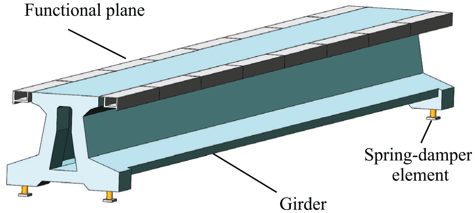
The TR08 model maglev trains are in operation on the SML. These vehicles consist of three principal components: carriages, bogies, and electromagnets. The carriages are connected to the bogies, maintaining a rail-hugging configuration as illustrated in Figure 1. The suspension electromagnets are positioned beneath the guideway. In operational conditions, the energized electromagnets interact with the functional planes embedded in the track, producing an electromagnetic force that achieves the levitation of the vehicle.

Schematic diagram of a maglev V/GC system in SML.
To facilitate the analytical modeling of maglev vehicles, the following assumptions have been made in this study:
The primary components of the maglev vehicle are considered rigid bodies, and each component has a small displacement.
Given that the vertical dynamic performance of the maglev V/GC system is primarily influenced by vertical vibrations, this study focuses exclusively on the vertical vibration of the vehicle body and guideway girder.
The masses of the bogies and carriages are assumed to be uniformly distributed across the associated spring-damping elements.
In the EMS maglev train mechanics calculation model, the train is typically represented by a simplified configuration comprising one carriage, four bogies, and eight suspension electromagnets. 21 The carriage is linked to the four bogies via eight springs and dampers, constituting the secondary suspension system. Each bogie, in turn, is connected to two suspension electromagnets through a pair of springs and dampers, respectively. Collectively, the four bogies and eight electromagnets, interconnected by eight springs and dampers, constitute the primary suspension system, as depicted in Figure 2. Drawing from the actual structure of the train, this paper develops a 2D, 18 Degrees of freedom (DOFs) high-speed maglev train model, 22 presented in Figure 3.

The dynamic model of TR08 maglev train.

The geometric model of TR08 maglev train.
The model attributes one vertical displacement and one pitching rotation to the carriage and each bogie. Each magnet is assigned a single vertical displacement. The DOF vector for an individual vehicle is denoted by equation (1).

Carriage dynamic formulation
Based on the dynamic model of the maglev train, the dynamic equation for the carriage is formulated and presented as equation (2):

where

where
Bogie dynamic formulation
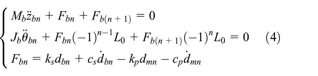
where

Electromagnet dynamic formulation

where
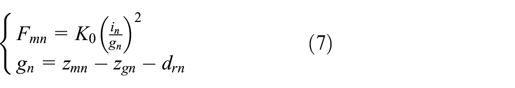
where
By integrating equations (2)–(6), we derive the matrix equations governing a maglev vehicle with 18 DOFs.

where the matrices
Guideway model
Drawing on prior research and actual model data,
10
this study develops a finite element model of the guideway, treating the girder unit as a two-dimensional Euler-Bernoulli beam element. The guideway is modeled as a simply supported girder bridge with a span of 24.768 m, as depicted in Figure 4. The girder is connected to its supports through spring-damper elements. The vertical stiffness is determined to be

where

where

The configuration of the guideway.
In the formulation of the guideway structure’s vibration equation, the mass matrix

where
Irregularity model
The vertical surface of the functional plane experiences inevitable deviations from its ideal geometric position due to track surface unevenness, manufacturing tolerances, and environmental variations. This deviation is termed “vertical irregularity,” and it significantly influences the dynamic response of the vehicle. To characterize the geometric variability of the guideway girder’s surface irregularities, this study employs the power spectral density function (PSD). Over recent years, numerous investigations have been conducted on track irregularities within the maglev transport sector.5,11,23,24 Notably, Shi et al. 3 developed a power spectrum model for high-speed maglev systems using data from the SML, a model that has gained broad acceptance in the field. Based on this research, this paper generates irregularity sample data utilizing the track PSD function, as illustrated in equation (13):

where f represents the spatial frequency. The wavelength range considered spans from 1 to 50 m. The parameters A, B, C, D, E, F, and G are characterization coefficients that define the PSD function and are detailed in Table 1.
Parameter for the PSD function.

Vehicle/guideway coupled model
Utilizing equations (8) and (11), the dynamic equation for the maglev V/GC system is formulated.

Addressing the solution of these dynamic equations involves tackling a nonlinear, time-varying system, specifically under the influence of the electromagnetic forces resulting from the one-dimensional magnetic-track interaction. This challenge is addressed using an incremental iterative algorithm based on the Newmark-
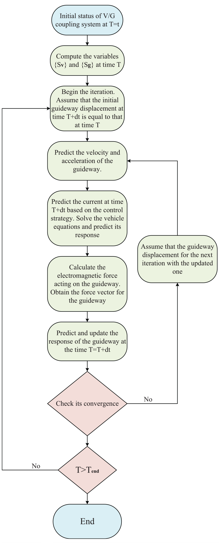
The flow chart of solving the V/GC model.
Parameters for the V/GC system.

Control model
The electromagnetic force serves as a critical medium for coupling the vehicle to the guideway in a maglev system. The implementation of an effective control strategy are essential, as they directly influence the accuracy of the simulation and the dynamic performance of the V/GC system. 25 In this section, we design a BSC algorithm for the V/GC system. To address the high precision requirements and computational complexity of the traditional backstepping algorithm and to enhance its robustness, we combine BSC with a fuzzy neural network, developing a BFNNC algorithm.
Backstepping control
The BSC algorithm is a sophisticated nonlinear control strategy, known for its effectiveness in addressing complex nonlinear control challenges. In this study, the objective of the suspension controller is to maintain the electromagnet’s suspension gap at a stable nominal value of 10 mm. To achieve this, we rewrite the equation (6). Define the input variable of the system:

Design a virtual control and define the error equations.

where
Step 1: Define the first Lyapunov function candidate as follow:

The derivative of it can be expressed as follows:

Define the virtual control law

where

Step 2: Define the second Lyapunov function candidate as follow:

The derivative of it can be expressed as follows:

Differentiating the

Combining equations (22) and (23),

Step 3: The feedback control law can be designed as:
where

According to the Lyapunov stability criterion, the trend of the system’s behavior can be described by constructing a Lyapunov function V based on the system. If V is positive definite at the equilibrium point and its derivative is negative definite in the neighborhood around the equilibrium point, the system states will gradually approach the equilibrium point over time, thereby achieving asymptotic stability. Since
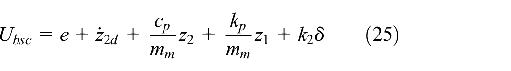
Step 4: Rewritten equation (25), the control law can be transformed as:

Therefore, the realistic current value in control system can be expressed as:

Backstepping fuzzy-neural-network control
Based on the analysis in the section “Backstepping control,” we can conclude that the system stability can be guaranteed theoretically when the BSC law (28) is adopted. However, selecting control parameters that yield the desired simulation outcomes can be challenging and often necessitates significant expertise. Furthermore, the control law relies on precise data for virtual control values e and
To address these limitations and enhance both the control performance and the robustness of the system, while also minimizing the reliance on highly accurate model data, this section introduces the design of the BFNNC strategy. This approach integrates the control efficacy of BSC with the inferential capabilities of the FNN. FNN harnesses the adaptive learning capabilities and logical computation of neural networks, 27 alongside the fuzzy reasoning of fuzzy systems 28 and the human-like decision-making processes of expert systems. 29 This integration enables the control system to achieve satisfactory performance without relying on highly precise model data, instead leveraging the computational logic of expert systems and neural networks. 30 The architecture is detailed in Figure 6.

Block graph of BFNNC system.
The Variable Transformation 1 module translates input parameters into control vectors e and
The FNN leverages an Adaptation Laws model to autonomously fine-tune the weights and the membership functions of the fuzzy subsets. Figure 7 illustrates the structure of a four-layer FNN, which includes an input layer, a fuzzification layer, a fuzzy rule layer, and an output layer. The input layer corresponds to the input vector:

Structure of the four-layer FNN.
where (

where

where

where

where

The approximation error can be linearized using Taylor’s theorem, leading to an error expansion expression:
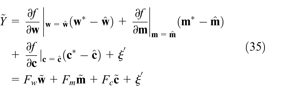
where
If (

If (
If (

If (

If (

If (

where
According to Lyapunov’s stability criterion and Barbara’s theorem, If
To ensure the convergence of the BFNNC, specifically
The time differentiation of

According to the equation (32), one can get that

Using equations (15), (27), and (34), the above equation can be rewritten as


Substituting equation (47) into equation (43) yields:

where
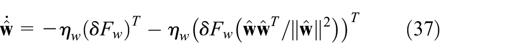
If the adaptation law for
When the condition of the equation (36) are satisfied,
When the condition of the equation (37) are satisfied,

As
If the adaptation law for
When the condition of the equation (38) are satisfied,

When the condition of the equation (39) are satisfied,

As
If the adaptation law for
When the condition of the equation (40) are satisfied,

When the condition of the equation (41) are satisfied,

As
Since
Validation
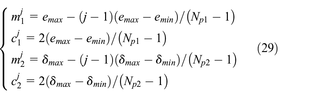
To verify the reliability of our numerical model, this study compares simulation outcomes with experimental data from the SML. The guideway and vehicle parameters within the V/GC model adhere to the configurations detailed in actual data. 10 The selection of parameters for both the BSC scheme and the BFNNC strategy is optimized for stability and control performance. The fuzzy neural network architecture comprises 2, 6, 9, and 1 neurons corresponding to the input layer, fuzzification layer, fuzzy rule calculation layer, and output layer, respectively. The fuzzification layer categorizes each input signal into three sets: N (negative), Z (zero), and P (positive), resulting in nine fuzzy rule units. The output layer utilizes a sigmoid activation function to synthesize and defuzzify the fuzzy signals. Inter-layer weight values between the fuzzification and fuzzy rule layers are initialized to 1, while the weights from the fuzzy rule layer to the output layer are assigned random initial values between 0 and 1. Each electromagnet is controlled independently.
The simulation device includes a train consisting of five vehicles and four simply supported beam bridges, each spanning 24.768 m. Figure 8(a) illustrates the simulation of a maglev train traversing the second span at a speed of 430 km/h, employing both the BSC and BFNNC control algorithms. For validation, the vertical displacement at the mid-span of the second simply supported girder is compared against experimental data. 31 The simulation results closely match the experimental measurements, with a peak displacement of 1.55 mm from the experimental data, 1.59 mm from the BSC scheme, and 1.60 mm from the BFNNC strategy, yielding relative errors of 2.58% and 3.22%, respectively. Figure 8(b) compares the coefficient of impart of variation for vertical displacement at the mid-span of the second span against measured values 23 across a speed range of 50–350 km/h. The control algorithms exhibit a consistent trend with the measured data, with a notable deviation observed at 125 km/h, potentially attributable to measurement errors. It can seen that it is in reasonable agreement with the result of the field test.
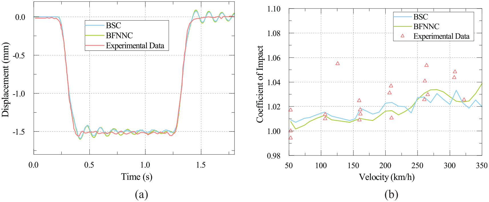
Comparison between the simulation data and experimental data of the middle span of the bridge: (a) bridge vertical displacement (v = 430 km/h) and (b) coefficient of impact (v = 50–350 km/h).
Case studies
This study simulates and analyzes the dynamic responses of the V/GC system under two distinct control algorithms: BSC and BFNNC. Comparative analysis of the simulation results across various operating conditions reveals that the BFNNC strategy outperforms the BSC strategy in terms of control effectiveness and robustness.
Control performance
The suspension gap variation amplitude is crucial for train operational safety, as excessive fluctuations can elevate the risk of collision, especially during high-speed operations. Figure 9(a) illustrates the suspension gap variation for the No.1 electromagnet of the head vehicle at a train speed of 430 km/h. The BSC system’s suspension gap fluctuates between 7.97 and 11.65 mm, whereas the BFNNC system’s suspension gap varies from 8.85 to 10.83 mm, indicating a 49.1% reduction in variation amplitude for the BFNNC strategy. Figure 9(b) presents similar data for the No.1 electromagnet of a middle vehicle, showing that the BFNNC system’s suspension gap fluctuates between 9.03 and 10.81 mm, compared to the BSC system’s range of 8.06–11.49 mm. Initially, from 0 to 0.42 s, the middle vehicle has not yet entered the bridge, maintaining a constant suspension gap. Upon the middle vehicle’s entry onto the bridge, the BFNNC strategy’s fuzzy control capabilities ensure minimal variation in suspension gap across different vehicles, in contrast to the BSC system. The reason for the bigger dynamic response of the head car is that it experiences a significant impact load when entering the bridge. The vehicle’s acceleration amplitude and spectral characteristics are closely related to ride comfort. Figure 10(a) depicts the acceleration variation of the head vehicle as it traverses the bridge at 430 km/h. The head vehicle passes over the bridge from 0 to 1.04 s. It has been completely off the bridge between 1.04 and 2 s. The BFNNC strategy results in lower vehicle acceleration amplitude and high-frequency vibration compared to the BSC system. The Sperling index, a key metric for evaluating ride comfort, is found to be 1.3665 for the BSC system and 1.3564 for the BFNNC system. Figure 10(b) displays the acceleration profile of a middle car crossing the bridge at 430 km/h. Between 0 and 0.42 s, the middle vehicle has not yet entered the bridge. It is actively traversing the bridge from 0.42 to 1.46 s. Subsequently, from 1.46 to 2 s, the vehicle has been completed off the bridge. The Sperling index values are 1.3647 for the BSC system and 1.3582 for the BFNNC system. The BFNNC strategy’s superior robustness prevents an increase in the index of running stability due to bridge vibrations. In both methods, the index remains below the highest requirement of the ride index
32
(

Variation of suspension gap of the No.1 electromagnet at different vehicles (430 km/h): (a) head vehicle and (b) middle vehicle.

Variation of the vehicle vertical acceleration at different vehicles (430 km/h): (a) head vehicle and (b) middle vehicle.
System dynamic responses at different operating speeds
Given the ongoing development of high-speed maglev transportation technology, a thorough analysis of the dynamic responses within the V/GC system across a range of operating speeds is essential. This analysis is crucial to ascertain the system’s safety and stability at both special and higher speeds. Therefore, this study analyzes the dynamic responses of both the guideway girder and vehicle.
The amplitude of guideway vibration, including deflection and acceleration, is pivotal to the structural safety of the entire system. Therefore, constraining the dynamic responses of the guideway girders is vital for ensuring train safety and ride smoothness. Typically, the midspan experiences the most significant vertical displacement and acceleration. Figure 11(a) illustrates the maximum deflection at the mid-span of the second bridge as a train traverses it at speeds varying from 200 to 800 km/h. The deflection generally increases with speed, maintaining a stable trend between 400 and 550 km/h, beyond which it escalates sharply. Despite the BFNNC strategy system exhibiting slightly larger girder displacements, the deflection amplitude remains within the acceptable limit 33 (L/4800 = 5.16 mm) even at 800 km/h. Figure 11(b) depicts the maximum vertical acceleration at the mid-span of the second bridge over the same speed range, which also increases with speed and remains within the safety limit (0.35g) at 800 km/h. In conclusion, these observations indicate that both control algorithms satisfy safety limits for bridge crossings up to 800 km/h.

Some key dynamic response amplitudes of the second bridge at mid-span at different vehicle speeds: (a) vertical displacement and (b) vertical acceleration.
The vehicle’s acceleration amplitude and index of running stability are critical indicators of ride comfort. Figure 12(a) presents the acceleration amplitude of the head vehicle as it passes through the bridge at speeds ranging from 200 to 800 km/h. The BFNNC strategy demonstrates better performance in the 200–500 km/h range. A distinct peak in the maximum acceleration amplitude is observed around 350 km/h, attributed to the vehicle’s driving frequency nearing the second-order natural frequency of the guideway, inducing resonance. Figure 12(b) displays the Sperling index variation as the head vehicle crosses the bridge at various speeds. The BFNNC strategy system’s index of running stability surpasses that of the BSC scheme system at high speed operation (550–800 km/h). The Sperling index peaks around 400 km/h. It increases with speed in high speed operation. However, both systems meet the highest requirement of the ride index for vehicle operations below 800 km/h.

Some key dynamic responses of the head vehicle at different speeds: (a) the amplitude of the vertical acceleration and (b) sperling value.
Robustness performance
During the actual operation of maglev trains, various factors such as passenger movement, wind loads, and unforeseen events can introduce unknown interference loads into the V/GC system, potentially compromising train safety. Consequently, the suspension control algorithm must exhibit robustness to handle these disturbances effectively. This section evaluates the robustness of two control algorithms—BSC and BFNNC—by analyzing their performance under step and sinusoidal load disturbances at an operational speed of 430 km/h.
Step loads, a common form of perturbation, are widely utilized in robustness testing due to their pronounced impact and computational efficiency.
34
In this study, a step disturbance with varying amplitudes is applied to each electromagnet from 0.4 to 0.8 s to investigate its effect on the suspension gap of the head vehicle. The impact of different step load amplitudes on this suspension gap is shown in Figure 13(a) and (b). Results indicate that while the BSC system fails to satisfy safety requirements for step loads exceeding 0.05

Variation of suspension gap of No.1 electromagnet on the head vehicle under different amplitude step interference forces at both control strategies (430 km/h): (a) BSC and (b) BFNNC.

Variation of suspension gap of No.1 electromagnet on the head vehicle at step interference load with amplitude 0.1
Sinusoidal loads, which can approximate any load profile via Fourier’s theorem, are also considered in this analysis. A sinusoidal disturbance with an amplitude of 0.1

Variation of suspension gap of No.1 electromagnet on the head vehicle under different frequency sinusoidal interference forces at both control strategies (430 km/h): (a) BSC and (b) BFNNC.

Variation of suspension gap of No.1 electromagnet on the head vehicle at sinusoidal interference load with amplitude 0.1
In conclusion, the BFNNC strategy effectively integrates the control precision of the BSC scheme with the inferential capabilities of the FNN, offering superior control performance and robustness.
Conclusion
This study presents the design and application of the BFNNC strategy for a high-speed maglev suspension control system, contrasted with the BSC scheme. A systematic analysis of the control performance under high-speed operations, guideway responses, vehicle responses at varying speeds, and robustness against different disturbance loads has led to the following conclusions:
The V/GC model developed in this research closely aligns with real-world scenarios. The BFNNC strategy demonstrates superior control performance compared to the BSC scheme. Specifically, at the maximum operational speed of 430 km/h, the suspension gap fluctuation of the head vehicle is reduced by 49.1% with the BFNNC strategy, and the Sperling index is also slightly lower. For the middle vehicle, the BFNNC strategy reduces suspension gap variation by 48.1% and lowers the Sperling index.
The guideway’s maximum vertical displacement and acceleration generally increase with train speed, with a notable escalation beyond 550 km/h. Despite the BFNNC strategy exhibiting slightly higher vertical displacements, it remains within safety limits at all speeds. During operations between 200 and 400 km/h, the BFNNC strategy significantly outperforms the BSC scheme in terms of head vehicle acceleration amplitude. The Sperling index correlates positively with speed in the high-speed range (550–800 km/h). Resonance occurs around 350 km/h as the vehicle’s driving frequency approaches the bridge’s second-order natural frequency, leading to extreme values in acceleration amplitude and index of running stability. Both control algorithms maintain safety within the dynamic responses below 800 km/h.
The suspension gap variation amplitude increases with the rise of step disturbance loads. Under a 0.1
(iv) Under a 5 Hz sinusoidal load with an amplitude of 0.1