Rolling trajectory generation for autonomous forklifts based on task time constraint

Abstract

As the demand for operational efficiency in intelligent factories and logistics systems continues to increase, trajectory planning for autonomous forklifts has become a critical technological challenge. In this paper, we propose a Task-Time Constrained Trajectory Rolling Planning (TTRP) approach that ensures timely task completion despite unforeseen circumstances. The TTRP method calculates time intervals between waypoints based on task time constraints and the forklift’s kinematic and dynamic models. By employing cubic spline interpolation, it replans the remaining trajectory after unplanned stops, ensuring smooth transitions and adherence to task time constraints. We validated the TTRP method using a ROS-based Gazebo simulation environment. Simulation results indicate that TTRP significantly improves trajectory smoothness and stability compared to traditional quintic polynomial interpolation methods. Specifically, TTRP reduces maximum jerk by up to 89.7%, decreases the standard deviation of acceleration by 88.1%, and lowers maximum speed variation by 61%. These findings demonstrate that TTRP efficiently generates smooth, feasible trajectories that meet the kinematic, dynamic, and task time requirements of autonomous forklifts in intelligent factory environments.

Introduction

Automation in manufacturing is necessary for the emergence of industry 4.0. Therefore, there is a need for innovation and development of satisfactory methods. ¹ As new production concepts emerge, emphasizes are made on the flexibility requirement of the operation of production lines and logistic systems. The pursuit of flexibility and product refinement in intelligent factories are extremely crucial ² because goods handling in the factory is often highly connected with the production and assembly line. ³ The connection between robot task navigation, factory production, and assembly line, directly affects a factory’s economic profit. To further improve production and goods handling efficiency of the whole factory, higher requirements need to be put in place for logistic robot navigation systems. Navigation systems need to meet high precision requirements such as safety in goods handling and prompt arrival time to maintain the work speed of the production line.

Trajectory generation is a crucial feature of autonomous mobile robots,^4,5 which involves not only collision-free path planning in complex environments but also trajectory tracking of the path in various real-world situations. Trajectory generation^6–8 usually refers to the generation of a trajectory containing pose information, motion control parameters, and time stamps based on the collision-free space in an environment with obstacles. Among these, the setting of motion control parameters and time stamps is the research focus of trajectory generation. Also, trajectory generation is the basis of a stable robot trajectory-tracking control.

At present, however, the optimal strategy used in the trajectory generation module of navigation tasks is usually based on time optimization, which takes into account the least time to execute the trajectory given a robot’s kinematic and dynamic constraints. ⁹ Such approach does not impose completion time constraints on navigation tasks, so the robots only reaches the target point with the fastest velocity available. In a multirobot workspace scenario, the optimum production speed of the whole production line will not be maintained or even reached. Moreover, if the robot accidentally moves into a safety zone during the execution of a navigation task, it will need to stop and re-plan its trajectory. This will result to failure in reaching the target point at the specified time. Robotic navigation based on task time constraint, requires the system to calculate the executable time of the remaining path according to the given total time and obstacle-stopping time (given related expected or unexpected occurrences) of the task. The task-time constrained trajectory rolling planning (TTRP) method ensures that the robot is able to regenerate its trajectory, enabling prompt arrival at the task target point after stoppage due to obstacle avoidance or safety zone encroachment. To account for task time requirements during trajectory planning, this paper makes the following significant contributions:

• A trajectory planning method based on task completion time constraint is proposed.

• The proposed method plans a trajectory that satisfies the kinematic, dynamic, and navigation task execution time constraints of the robot.

• The method can adaptively plan new trajectories based on the remaining path and task completion time given unexpected events such triggered safety mechanism (stop) during navigation.

The content of this paper is organized as follows: The second section discusses related work. The third section introduces in details, the robot TTRP method. The fourth section provides details on the experimental verification of the method proposed in this paper, and presents the results showing the effectiveness and robustness of the method. The fifth section presents the conclusion, and puts forward prospects for future research according to the shortcomings of the proposed method in this paper.

Related works

The trajectory generation is an essential research topic concerning the advancement of mobile robot technology. Trajectory generation involves the process of obtaining a trajectory path containing state information and control information according to a specific performance index such as distance, time, and energy, and according to the specific requirements of the task after kinematic and dynamic analysis. In recent years, many scholars have proposed various trajectory generation methods which can be mainly classified into optimization, spline curve, and unique curve based generation methods.

Regarding trajectory smoothing based on optimization methods, the trajectory planning problem is modeled as a quadratic programming (QP) problem with constraints. The optimization function can be snap, jerk, acceleration, their combination or any other function that can be formulated in pTQp form. Their constraints usually include equality constraints and inequality constraints.^10,11 Mellinger and Kumar ¹² proposed a trajectory optimization approach using polynomial parameterization, which ensured smooth transitions but lacked time-adaptive re-planning capabilities in unforeseen interruptions. Xu et al. ¹³ proposed a hybrid trajectory optimization method designed to generate efficient, stable, and smooth terrain traversal for articulated tracked robots. This method integrates a kinematic model with an optimization-based trajectory planning framework and employs a two-stage optimization process. The trajectory is refined using a nonlinear programming approach to minimize metrics such as jerk and energy consumption, thereby ensuring trajectory smoothness and stability. However, the method’s reliance on precomputed global paths limits its adaptability to dynamic task time constraints, such as emergency stops or unexpected obstacles. This limitation highlights the need for further advancements to enhance its applicability in real-time and dynamically changing environments. These studies highlight the critical importance of real-time adaptability to task time constraints.

Spline curves are widely used in the field of mobile robot trajectory generation because they have the advantage of continuous curvature. That is, there curvature is still continuous at the nodes of adjacent curve segments. Walambe et al.^14,15 proposed a trajectory generation approach based on the spline method, which overcame the parameter singularity generated by the differential flatness method. When cubic polynomial interpolation is used, the spline trajectory also considers the singular points in the optimization process. Zhou et al. ¹⁶ improved the smoothness and clearance of generated trajectories through B-spline optimization. By expressing the final trajectory as a non-uniform B-spline, the iterative time adjustment method was adopted to ensure dynamic feasibility, but this method was time-consuming in a multi-robot environment.

In recent years, unique curves have also been applied to the trajectory generation of mobile robots. For instance, Dubins curve was used to connect any two way-points in Oliveira et al. ¹⁷ However, the main disadvantage of the generated paths is that their curvature is discontinuous. Therefore, the robot traveling along this path must stop at each discontinuous point (e.g. at the transition between a straight line and an arc segment), read just the wheel direction, and then move forward. In order to overcome this problem, Chen et al. ¹⁸ proposed a method which produced paths with continuous curvature by using the Dobbins curve and Fermat spiral curve. Similar to the convolution curve, the curvature of the Fermat spiral curve changes with the arc length of the curve. This kind of curve provides a smooth transition of continuous curvature and a minimum length curve with a given jerk limit. However, there is no closed-form expression for the position along the cyclotron path, so an approximation and lookup table is needed.

Also, trajectory planning research has increasingly incorporated task time constraints as a central focus, significantly contributing to enhancing the adaptability of mobile robots in dynamic environments and improving task completion efficiency. Shen et al. ¹⁹ proposed a comprehensive and time-optimal trajectory planning algorithm with path constraints. By simultaneously accounting for dynamic limitations of torque and velocity, this method achieves real-time planning with theoretically proven completeness and time-optimality. Compared to traditional methods, this algorithm demonstrates notable advantages in terms of time efficiency and theoretical feasibility in trajectory planning. However, its adaptability to highly dynamic and complex environments remains an area for further exploration, as the study primarily addresses predefined path conditions. Moreover, Tao et al. ²⁰ introduced a deep reinforcement learning-based trajectory planning framework specifically addressing time constraints in dynamic environments. Leveraging neural networks to learn planning strategies in complex environments, this approach exhibits strong adaptability in scenarios with high environmental dynamism. Nevertheless, the training of reinforcement learning models demands substantial amounts of data and time, posing challenges for their rapid deployment in new environments. Recent studies indicate that while the integration of task time constraints has made significant strides, challenges persist in achieving real-time adaptability in dynamic environments, ensuring trajectory smoothness, and maintaining the precision of time constraints.

The above methods can generate smooth trajectories with continuous velocity and acceleration. However, the following problems still exist: First, there is a significant difference between the generated trajectory and path, and in some instances there may even be a “knot” phenomenon in the trajectory. Second, the obtained trajectories may exhibit excessive acceleration, which sometimes exceeds the maximum acceleration limit of the robot. To achieve control feasibility, it is usually necessary to check the trajectory after generation and ensure that it meets the maximum velocity, maximum front wheel angular velocity, and maximum acceleration limits of the robot. However, generating the trajectory and carrying out the feasibility test require significant work. The fundamental reason for the above problems lies in the unreasonable time allocation between destinations. Reasonable time allocation is key to obtaining a smooth and feasible trajectory. Finally, the above methods cannot solve trajectory-planning problems that satisfy task time-allocation constraints, particularly when the triggering of robotic safety obstacle avoidance leads to the loss of allocated navigation task execution time. To satisfy the task time allocation constraint, it is necessary to regenerate the trajectory of the remaining paths according to the original-arrival-target time.

To solve the above problems, this paper proposes a four-step TTRP method that meets the task time constraints. Firstly, the minimum time between each way-point is calculated according to the kinematic and dynamic constraints of the robot to get the minimum time for the whole task path. Secondly, the initial way-point timestamp is redistributed according to the task time constraint. Thirdly, the cubic spline curve is used to interpolate each way-point and the corresponding timestamp information smoothly. A smooth trajectory satisfying the robot’s kinematic, dynamic, and task arrival time constraint is then obtained. Finally, when the safety obstacle avoidance is triggered during task execution, the trajectory is roll generated to meet up with the allocated task time constraint.

Task-time constrained trajectory rolling planning

Emerging intelligent factories^21,22 have higher requirements regarding the precision, safety, and reliability of unmanned transport robots pertaining the execution of logistics operations. In addition to meeting the requirements of the navigation system for handling goods, the speed of goods transportation is also a crucial factor. Also, the generation of high-quality trajectory is essential for achieving high-precision trajectory-tracking control. ²³

For advanced factory, a task scheduling system sends robot navigation instructions according to the production task arrangement, which consists of the start and end locations, and the completion time of the navigation task. ²⁴ After obtaining the start and end locations, the robot navigation system searches for, and optimizes the global path to obtain a safe, smooth, and high-precision path composed of discrete waypoints. Each way-point contains the robot’s pose x, y, θ and steering angle information ϕ.

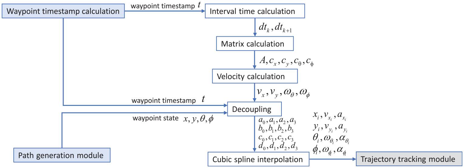
The algorithm flowchart for the trajectory rolling generation method is shown in Figure 1. It mainly consists of two components: (a) calculating way-point timestamps and (b) creating smooth way-point control sequences.

Figure 1.

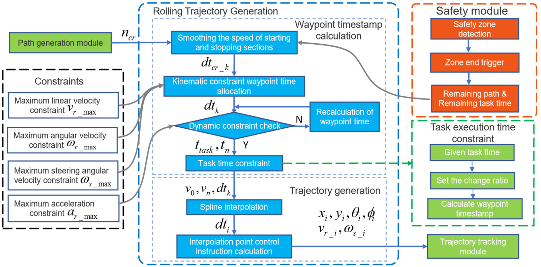
Rolling trajectory generation method block diagram with incorporated constraints consisting of minimum time completion, linear velocity, maximum vehicle angular velocity, maximum steering angular velocity, and maximum acceleration.

The primary function of the first main component is to process the generated path and determine the timestamps for each way-point. Each way-point K, comprises of the corresponding state of the robot s _k (pose x, y, angle θ, and steering angle ϕ), control command u _k (including the forklift linear velocity v _r , steering wheel rotation angular velocity ω _s ), and timestamp t _k . Initially, the way-point timestamp was determined by considering the robot’s maximum linear velocity, angular velocity, and steering wheel rotation angular velocity constraints. Subsequently, the generated timestamp was checked against the maximum acceleration constraint. Finally, the way-point timestamp was obtained, ensuring that the robot’s kinematics, dynamics, and minimum task completion time constraints were met.

The second component of the system employs the spline curve interpolation method to create a smooth trajectory between way-points that meets the robot’s control precision and other requirements. The spline interpolation function generates the interpolation points based on the state and way-point timestamp information. Subsequently, a set of smooth control sequence of the trajectory is generated. Finally, if the robot is in operation and encounters obstacles, the navigation system generates the trajectory for the remaining path in a roll-wise manner to satisfy the task time constraint.

Forward kinematics of the forklift robot

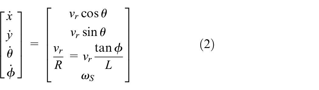
In a factory environment, forklifts primarily transport cargo at lower speeds, causing them to be subject to relatively low lateral forces. Therefore, a simplified kinematic model of the forklift was established to satisfy the design requirements for trajectory tracking. For the established model, we assumed that (a) the forklift did not slip while traveling, (b) the structure of the forklift was rigid, (c) there were no wheel deformations, (d) the motion of the forklift on the ground plane did not involve significant pitching or tilting, and (e) there was only rolling (rotatory) contact between the wheels, that is, there was no lateral sliding phenomenon. The kinematic model of the forklift is illustrated in Figure 2.

Figure 2.

Vehicle kinematics model.

In Figure 2, XOY is the world coordinate system, (x, y) represents the center coordinates of the rear wheel, O is the instantaneous center of rotation of the forklift, L denotes the wheelbase length of the vehicle, v _r denotes the linear velocity from the center of the rear axle toward the moving direction of the forklift (rear wheel linear velocity will be used in future references), ω denotes the angular velocity of the steering wheel, v _s denotes the linear velocity of the vehicle’s front wheel, and ϕ and θ represent the front-wheel’s angle of rotation and vehicle heading angle, respectively. R is the turning radius of the vehicle given in equation (1)

$$R=\frac{L}{\tan \varphi }$$

(1)

The vehicle kinematic model is given as

$$\begin{array}{c}\multicolumn{1}{c}{\left[\begin{array}{c}\stackrel{·}{x}\hfill \\ \multicolumn{1}{c}{\stackrel{·}{y}}\\ \multicolumn{1}{c}{\stackrel{·}{\theta }}\\ \multicolumn{1}{c}{\stackrel{·}{\varphi }}\end{array}\right]=\left[\begin{array}{c}{v}_r\cos \theta \hfill \\ \multicolumn{1}{c}{v_r\sin \theta }\\ \multicolumn{1}{c}{\frac{v_r}{R}=v_r\frac{\tan \varphi }{L}}\\ \multicolumn{1}{c}{{\omega }_S}\end{array}\right]}\end{array}$$

(2)

Inverse kinematics of the forklift robot

Inverse kinematics (IK) is essential in the control of forklift robots, allowing for the calculation of control inputs (such as steering angles and velocities) to ensure accurate motion along a desired trajectory. For the single-steering-wheel forklift model, the inverse kinematics framework is established and mathematically formulated to address trajectory tracking requirements.

To calculate the steering angle ϕ, the geometric relationship between the current vehicle position (x, y) and the target waypoint (x _t , y _t ) is first determined. The direction angle α to the target is computed as:

$$\alpha =\mathrm{atan}2(y_t-y,x_t-x)$$

(3)

The required steering angle ϕ can then be determined as:

$$\varphi ={\tan }^{-1}\left(\frac{L}{\sqrt{{(x_t-x)}^2+{(y_t-y)}^2}}\right)-(\theta -\alpha )$$

(4)

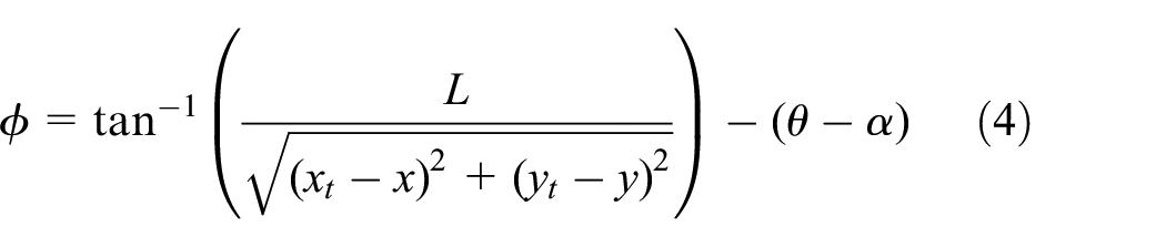
The use of the atan2 in equation (4) ensures correct calculation of α across all four quadrants, avoiding errors caused by traditional trigonometric functions such as acos, asin, or atan, which are limited to specific quadrants.

The instantaneous linear velocity of the rear wheel v _r is calculated based on the distance to the target waypoint:

$$v_r=k_v·\sqrt{{(x_t-x)}^2+{(y_t-y)}^2}$$

(5)

where k _v is a proportional gain factor. The linear velocity of the steering wheel v _s is given by:

$$v_s=\frac{v_r}{\cos (\varphi )}$$

(6)

The vehicle’s instantaneous angular velocity ω is derived from the linear velocity v _r and the turning radius R:

$${\omega }_r=\frac{v_r}{R}=\frac{v_r·\tan (\varphi )}{L}$$

(7)

The angular velocity of the steering wheel ω _s is computed as:

$${\omega }_s=\frac{{\varphi }_t-\varphi }{\mathrm{\Delta }t}$$

(8)

where Δt is the time step for trajectory updates.

The proposed inverse kinematics model ensures accurate calculation of the control inputs required for trajectory tracking in the forklift robot. The use of the atan2 function avoids quadrant-related errors inherent in traditional trigonometric functions, significantly improving the accuracy of angle calculations. Equations (3)–(8) form the core of the inverse kinematics framework, providing a robust theoretical foundation for precise trajectory control in dynamic environments. This method benefits from the kinematics solution approach based on exponential rotational matrices proposed by Ayiz and Kucuk, ²⁵ which provides a solid foundation for the theoretical framework.

Dynamics model

The dynamics model of the single-steering forklift extends its kinematic model by incorporating the effects of external forces and torques on the vehicle’s motion. The forklift is modeled as a rigid body with a mass M and a moment of inertia I, with the center of mass located at the vehicle’s centroid. The motion of the vehicle is governed by Newton’s second law, and the fundamental dynamics equations are as follows:

$$\begin{array}{c}M·\stackrel{··}{x}=F_x\hfill \\ M·\stackrel{··}{y}=F_y\hfill \\ I·\stackrel{··}{\theta }=\tau \hfill \end{array}$$

(9)

where F _x and F _y are the external forces acting along the x- and y-directions, respectively, and τ represents the torque about the vehicle’s center of mass. The terms $\stackrel{··}{x}$ , $\stackrel{··}{y}$ , and $\stackrel{··}{\theta }$ denote the linear accelerations in the x- and y-directions and the angular acceleration about the yaw axis, respectively.

To address practical operation requirements, physical and operational constraints are introduced to ensure the safety and controllability of the forklift’s motion. These constraints include:

• (1) Maximum linear velocity constraint v_{r_max}: The vehicle’s linear velocity is limited to v _r  ≤ v _r __max, preventing unsafe high-speed operation.

• (2) Maximum angular velocity constraint ω_{r_max}: The vehicle’s angular velocity satisfies ω _r  ≤ ω_{r_max}, ensuring stable rotation during turns.

• (3) Maximum steering angle constraint ϕ_max: The steering angle is restricted to |ϕ| ≤ ϕ_max, reflecting the mechanical limits of the steering mechanism and preventing oversteering.

• (4) Maximum steering angular velocity constraint ω_{s_max}: The rate of change of the steering angle is limited to |ω _s | ≤ ω_{s_max}, avoiding abrupt and excessive directional changes.

These constraints are naturally integrated into the dynamics model by bounding the control inputs F _x , F _y , and τ. For instance, F _x and F _y directly influence the linear accelerations and velocities, while τ is related to the steering angle ϕ and angular velocity ω _r . By restricting these control inputs within predefined limits, the dynamics model can effectively enforce the operational constraints.

In practical applications, these constraints are incorporated into trajectory planning algorithms, such as the Trajectory Time Rolling Planning (TTRP) method. This approach ensures that the generated trajectories are not only dynamically feasible but also adhere to the safety and operational limits of the forklift. By implementing these constraints, the forklift achieves stable and predictable behavior, even in dynamic and complex operational environments.

Way-point time allocation based on kinematics and time constraints

Time allocation directly affects the navigation task completion time, feasibility and smoothness of trajectory interpolation. Usually, the path way-points contain x, y, θ, ϕ state information but do not contain the control sequence information of the robot’s velocity and acceleration. The TTRP method computes the timestamp of each waypoint on the generated path by incorporating maximum velocity and acceleration constraints. Upon entering the path, the system initially computes the minimum task duration that satisfies the current kinematic constraints of the robot.

In order to meet the requirements of the actual industrial scene, the system calculates the task completion time factor according to the task time set by the user. Then, adjustments are made on the way-point timestamp in proportion to the time factor to account for the robot’s kinematics and task completion time. The way-point time allocation block diagram is shown in Figure 3. The system receives the generated path, constraints and task time, and outputs a trajectory with timestamp.

Figure 3.

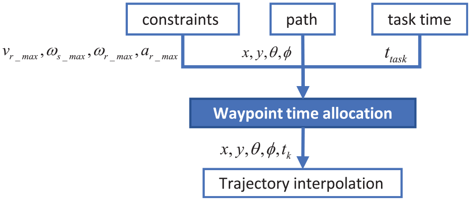
Way-point time allocation block diagram.

Determining way-point timestamp based on the kinematic constraints

In accordance with the robot kinematic model (Figure 2), a kinematic constraint was first established. ²⁶ Then the smoothed path containing control sequences and timestamps was generated. ²⁷

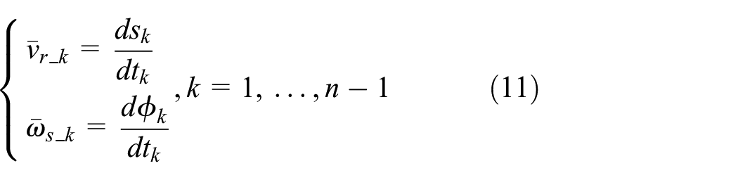
The time intervals between each way-points was calculated separately according to the maximum used time after the incorporation of the kinematic constraints. That is, dt_{νr_k}, dt_{ωr_k}, and dt_{ωs_k} are the time intervals between way-points derived from the robot’s maximum linear velocity, rotating angular velocity, and front wheel rotational velocity, respectively. dt _k is the largest value amongst dt_{νr_k}, dt_{ωr_k}, and dt_{ωs_k} representing the largest time between each way-points. The time interval calculations are detailed in equation (10).

$$\{\begin{array}{c}d{t}_{\mathrm{vr}\_k}=\frac{\sqrt{{(p(x_{k+1})-p(x_k))}^2+{(p(y_{k+1})-p(y_k))}^2}}{v_{r\_max}}\hfill \\ d{t}_{\omega r\_k}=\frac{\sqrt{{(p({\theta }_{k+1})-p({\theta }_k))}^2}}{{\omega }_{r\_max}}\hfill \\ d{t}_{\omega s\_k}=\frac{\sqrt{{(p({\varphi }_{k+1})-p({\varphi }_k))}^2}}{{\omega }_{s\_max}}\hfill \\ d{t}_k=max(d{t}_{\mathrm{vr}\_k},d{t}_{\omega r\_k},d{t}_{\omega s\_k})\hfill \end{array},k=1,\dots ,n-1$$

(10)

where p(x _k , y _k ) represents way-point location, p(θ _k ) denote position angle, and p(ϕ _k ), the front steering wheel rotation angle state value of the kth way-point. Given that the input path has n way-points, we take the positional difference ds _k of the kth waypoint as the euclidean distance between the point p(x _{k +1}, y _{k +1}) and p(x _k , y _k ). Also, the steering angle difference dϕ _k of the kth way-point was determined based on the difference between the steering angle p(ϕ _{k +1}) and p(ϕ _k ). As there may be variations in instantaneous velocity values within a way-point segment, an average is calculated for each segment. The average linear velocity ${\overline{v}}_{r\_k}$ and the average steering wheel rotation angular velocity ${\overline{\omega }}_{s\_k}$ of each segment were calculated as follows:

$$\{\begin{array}{c}{\overline{v}}_{r\_k}=\frac{d{s}_k}{d{t}_k}\hfill \\ {\overline{\omega }}_{s\_k}=\frac{d{\varphi }_k}{d{t}_k}\hfill \end{array},k=1,\dots ,n-1$$

(11)

where ${\overline{v}}_{r\_k}$ and ${\overline{\omega }}_{s\_k}$ are the way-point segment control velocity parameters. Similarly, an average linear acceleration ${\overline{a}}_{r\_k}$ is calculated according to equation (12) for each way-point segment on the trajectory. The ${\overline{a}}_{r\_k}$ control parameter was used for acceleration feasibility check to help reduce robot jittering or jerk caused by excessive acceleration and improve tracking accuracy.

$${\overline{a}}_{r\_k}=\frac{{\overline{v}}_{r\_(k+1)}-{\overline{v}}_{r\_k}}{d{t}_k},k=1,\dots ,n-1$$

(12)

Given that the robot has a maximum linear acceleration constraint of a_{r_max}, if the average acceleration of the kth segment satisfies ${\overline{a}}_k<a_{r\_max}$ , then the acceleration constraint condition is met. The feasibility check of the (k + 1)th segment average acceleration ${\overline{a}}_{k+1}$ can be performed subsequently. Otherwise, the time interval dt _k needs to be updated to satisfy the acceleration constraint. Since the positional difference ds _k is unchanged and ${\overline{a}}_{r+k}<a_{r\_max}$ must be satisfied, an update on dt _k can be performed according to:

$$d{t}_k=\frac{-{\overline{v}}_{r\_k}+\sqrt{{({\overline{v}}_{r\_k})}^2+2a_{r\_max}d{s}_k}}{a_{r\_max}}$$

(13)

Given that dt _k was updated, the average linear velocity ${\overline{v}}_{r\_k}$ and the average steering wheel angular velocity ${\overline{\omega }}_{s\_k}$ of each way-point would be recalculated according to equation (11). We set timestamp of the starting point of the path to 0, then update timestamps of all other way-points according to dt _k . The total time of the path is the timestamp of the last way-point t _n .

Velocity smoothing of the starting and stopping segments

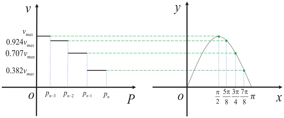
To mitigate the effects of abrupt acceleration in the start and stop segments of the trajectory, the time allocation in these segments was increased by implementing maximum velocity constraints that satisfy a sin curve. ²⁸ This smoothens the velocity profile of the relevant trajectory segments to achieve optimal trajectory tracking control. Here, we set a distance from the starting way-point and a distance before the ending way-point as smoothing segments. When the starting segment is smoothed, the relationship between the maximum velocity and time allocation of the robot has a sin function relationship and the robot’s velocity will begin at 0, and gradually increase to v_max. When decelerating smoothly in the stopping segment, the velocity of the robot will gradually decrease from v_max to 0. Assuming the total number of way-points in the smoothing segment is n _cr , considering the i _cr path segment, the corresponding maximum velocity of the segment is:

$$v_{\mathrm{cr}}(i_{\mathrm{cr}})=v_{\mathrm{cr}}(0)+(v_{\mathrm{cr}}(n_{\mathrm{cr}})-v_{\mathrm{cr}}(0))(\frac{i_{\mathrm{cr}}}{n_{\mathrm{cr}}}-\frac{1}{2\pi }\sin \frac{2\pi i_{\mathrm{cr}}}{n_{\mathrm{cr}}})$$

(14)

where v _cr (0) represents the starting velocity, v _cr (n _cr ) is the ending velocity. When the robot is located in the smoothing segments v _cr (0) = 0 and v _cr (n _cr ) = v_{r_max}. During the smoothing process, the system will set the maximum velocity smoothing coefficient between each way-points. The smoothing coefficient obeys the sin trigonometric function, as shown in Figure 4, where p _n represents the smoothed trajectory way-points.

Figure 4.

Starting segment velocity smoothing.

Conversely, on the ending smoothing segments, v _cr (0) = v_{r_max} and v _cr (n _cr ) = 0. The maximum velocity smoothing coefficient of the stopping segment is shown in the Figure 5.

Figure 5.

Stopping segment velocity smoothing.

After determining the smoothing coefficient, the time interval dt _k will be updated by v _cr (i _cr ) according to the obtained smooth linear velocity constraint of each waypoint segment (starting and stopping segment). For the kth way-point on the smooth segment, the time interval is given as:

$$d{t}_{\mathrm{cr}\_k}=\frac{v_{\mathrm{cr}}(n_{\mathrm{cr}})}{v_k}d{t}_k,k=1,\dots ,n_{\mathrm{cr}}-1$$

(15)

For the smooth path starting or stopping segments, the smoothing distance is calculated according to:

$$d{s}_{\mathrm{cr}}=\sum _{k=0}^{n_{\mathrm{cr}}-1}{\int }_{d{t}_{\mathrm{cr}\_k}}^{d{t}_{\mathrm{cr}\_k+1}}{v}_{\mathrm{cr}}\mathrm{dt}$$

(16)

Time allocation based on task-time constraints

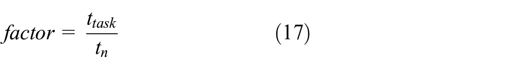
The system calculates or recalculates the timestamps of each way-point based on the execution task-time t _task given by the user. When the time t _task  ≤ t _n is sent as input, the robot would be unable to meetup with the requirement. Therefore, the robot would execute the task according to the corresponding control sequences and achievable minimum time of the path t _n . When the time t _task  > t _n is entered, the timestamp of each way-point will be reset according to the time set by the user. With a given user task-time t _task , the timestamp proportional changes at the way-points is defined as a factor expressed as:

$$\mathrm{factor}=\frac{t_{\mathrm{task}}}{t_n}$$

(17)

Therefore, the path way-point time intervals, dt _k , changes uniformly to dt_{task_k} and can be obtained by calculating:

$$d{t}_{\mathrm{task}\_k}=\mathrm{factor}\times d{t}_k,k=1,\dots ,n-1$$

(18)

The control command sequences between way-points can be updated according to dt_{task_k} according to equation (19).

$$\{\begin{array}{c}{v}_{r\_\mathrm{task}\_k}=\frac{\sqrt{{(x_{k+1}-x_k)}^2+{(y_{k+1}-y_k)}^2}}{d{t}_{\mathrm{task}\_k}}=\mathrm{factor}\times v_{r\_k}\hfill \\ {\omega }_{s\_\mathrm{task}\_k}=\frac{\sqrt{{({\varphi }_{k+1}-{\varphi }_k)}^2}}{d{t}_{\mathrm{task}\_k}}=\mathrm{factor}\times {\omega }_{s\_k}\hfill \end{array},k=1,\dots ,n-1$$

(19)

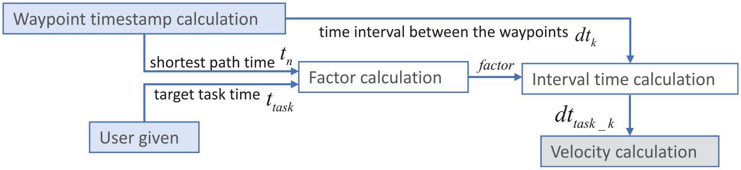
With equation (19), the task time of the path can be set according to the actual needs of the user. Consequently, the timestamp of the way-points are also adjusted to regulate the overall velocity of the robot. We calculated the timestamps to meet the task-time constraint according to the block diagram in Figure 6 and algorithm 1 below.

Figure 6.

Algorithm 1 block diagram.

Algorithm 1.

Trajectory generation algorithm.

Require: t n , t task , vr_k, ws_k, n, dt k Ensure: Updated velocities vr_task_k, ωs_task_k for k∈ {1, 2, …, n}

1: factor← CalProportional (t n , t task )

2: dttask_k← CalIntervalTime (factor, dt k )

3: fork = 1 to n do

4:   $v_{r\_\mathrm{task}\_k}\leftarrow v_{r\_k}\times \mathrm{factor}$

5:   ${\omega }_{s\_\mathrm{task}\_k}\leftarrow {\omega }_{s\_k}\times \mathrm{factor}$

6: end for

Algorithm 1 takes as input: shortest path time t _n , target task time t _task , number of way points n, control sequence parameters (v _r , w _s ) and time intervals between the way-points dt _k . Using the robot heading angle θ _k , v _r can be decomposed into v _xk and v _yk , while ω _s remains the angular velocity of the steering wheel rotation. Algorithm 1 first calculates a factor value based on the set task time and the shortest task time. The algorithm then adjusts the way-point interval time using dt _k in equation (18) when the task time is greater than the estimated (shortest) path time. From step 3 to step 5 (algorithm 1), the control sequence values of all way-points are readjusted proportionally based on the factor value (equation (19)).

Trajectory smoothing interpolation

Based on the spline curves, smooth interpolation points with fixed control periods were obtained using the trajectory way-points and their corresponding timestamps. We ensure the smoothness of trajectory interpolation points and reduced calculation complexity by using cubic spline curves to interpolate the trajectory way-points. ²⁹ The cubic spline curves interpolation approach make reasonable compromise between flexibility and calculation speed. Compared with higher-order splines, cubic spline interpolation needs less calculation, storage space, and is more stable. Again, compared with linear spline interpolation, the trajectory generated by cubic spline interpolation is smoother and more suitable for robot motion control. ³⁰

Conditions of trajectory smooth interpolation

Interpolation points generated by cubic spline include the state quantity s _i (i.e. pose p(x, y, θ) and heading angle p(ϕ)) and control sequence commands u _i (i.e. robot linear velocity v _r and front wheel rotational angular velocity ω _s ). ³¹ With a total of n waypoints and n − 1 way-point segments, n − 1 cubic polynomials were used to determine the trajectory parameters based on a regression approach. Finally a sequence of interpolation function was obtained.

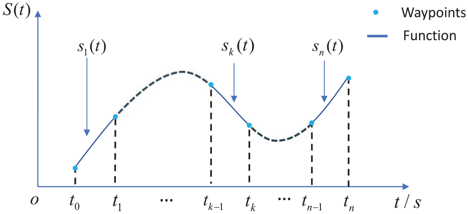
To perform trajectory tracking control at a stable frequency, the smoothed path was sampled equally based on uniform time intervals. We define the time dependent way-points function sequence of trajectory path as S(t) and the kth way-point segment as s _k (t). S(t) and s _k (t) are then used to determine the position and control sequence commands of all interpolation points according to equation (20).

$$\begin{array}{c}S(t)=\{s_k(t),t\in [t_k,t_{k+1}],k=0,\dots ,n-1\},\hfill \\ s_k(t)=a_{k0}+a_{k1}(t-t_k)+a_{k2}(t-t_k{)}^2+a_{k3}(t-t_k{)}^3\hfill \end{array}$$

(20)

The trajectory is smoothly interpolated using the cubic spline function which consists of four unknowns, that is, there are 4(n − 1) unknowns for the k way-point sections. Therefore, to solve the function coefficient, 4(n − 1) conditions need to be known. The conditions defined in this paper are as follows: (1) Every cubic spline function must pass through two path points at its extreme value, and there will be 2(n − 1) conditions; (2) If the velocity of the intermediate way-point is continuous, there will be (n − 2) conditions; (3) The acceleration of the intermediate way-point is continuous, and there will be (n − 2) conditions at this time. (4) There are two conditions for the velocity of the starting and ending points. At this time, the sum of the conditions is known as 4(n − 1), and the parameters of each trajectory can be obtained. The schematic diagram of interpolation conditions is shown in Figure 7.

Figure 7.

Interpolation function plot of way-point state quantity against time: (a) Condition-1: Pass through the first and last way-points of the track, (b) Condition-2: Continuity of first order derivative, (c) Condition-3: Continuity of second derivative, and (d) Condition-4: Velocity of the first and last way-points of the trajectory.

The corresponding formulas are as follows:

$$\{\begin{array}{c}{s}_k(t_k)=p_k,s_k(t_{k+1})=p_{k+1},k=0,\dots ,n-1\hfill \\ {\stackrel{·}{s}}_k(t_{k+1})={\stackrel{·}{s}}_{k+1}(t_{k+1}),k=0,\dots ,n-1\hfill \\ {\stackrel{··}{s}}_k(t_{k+1})={\stackrel{··}{s}}_{k+1}(t_{k+1}),k=0,\dots ,n-2\hfill \\ {\stackrel{·}{s}}_k(t_0)=v_0,{\stackrel{·}{s}}_{n-1}(t_n)=v_n\hfill \end{array}$$

(21)

where p _k represents any of the state quantities. The kth segment of the S(t) function is plotted in Figure 8.

Figure 8.

Function of the time-varying state.

Coefficient solution of interpolation function

The first and second derivatives of the function $s_k()$ is denoted as ${\stackrel{·}{s}}_k()$ and ${\stackrel{··}{s}}_k()$ . We set dt _k as the time in k, and if there is an acceleration continuity at the intermediate way-point, the coefficient can be substituted into equation (21) obtaining:

$$\begin{array}{c}\multicolumn{1}{c}{{\stackrel{··}{s}}_k(t_{k+1})=2a_{k2}+6a_{k3}d{t}_k=2a_{(k+1)2}}\\ ={\stackrel{··}{s}}_{k+1}(t_{k+1}),k=[1,n-2]\hfill \end{array}$$

(22)

Under these conditions, by multiplying the expressions a _{k 2}, a _{k 3}, a_(k+1)2 by (dt _k dt _{k +1})/2, we can get:

$$\begin{array}{c}d{t}_{k+1}{v}_k+2(d{t}_{k+1}+d{t}_k)v_{k+1}+d{t}_k{v}_{k+2}\hfill \\ =\frac{3}{d{t}_{k+1}d{t}_k}[{\mathrm{dt}}_k^2(s_{k+1}(t_{k+2})-s_{k+1}(t_{k+1}))\hfill \\ +{\mathrm{dt}}_{k+1}^2(s_k(t_{k+1})-s_k(t_k))]\hfill \end{array}$$

(23)

According to equation (23), the velocity v _k of each way-point can be obtained. Also, according to the velocity and state of the way-point, we can deduce:

$$\{\begin{array}{c}{s}_k(t_k)=a_{k0}=p_k\hfill \\ {\stackrel{·}{s}}_k(t_k)=a_{k1}=v_k\hfill \\ s_k(t_{k+1})=a_{k0}+a_{k1}d{t}_k+a_{k2}{\mathrm{dt}}_k^2+a_{k3}{\mathrm{dt}}_k^3=p_{k+1}\hfill \\ {\stackrel{·}{s}}_k(t_{k+1})=v_{k+1}\hfill \end{array}$$

(24)

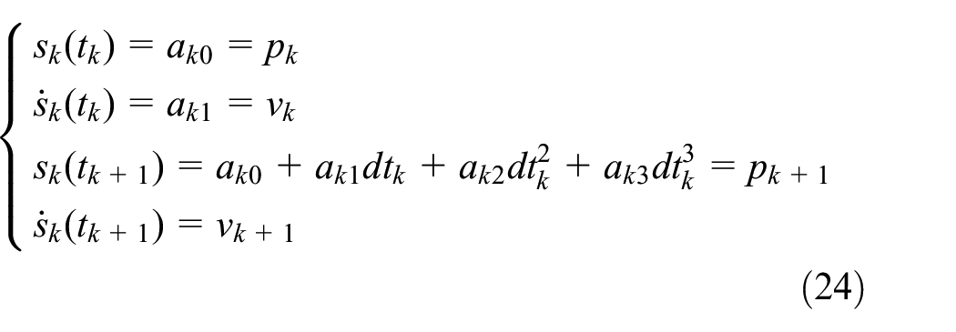
The coefficients of the cubic spline equation are as follows:

$$\{\begin{array}{c}{a}_{k0}=p_k\hfill \\ a_{k1}=v_k\hfill \\ a_{k2}=\frac{1}{d{t}_k}[\frac{3(q_{k+1}-q_k)}{d{t}_k}-2v_k-v_{k+1}]\hfill \\ a_{k3}=\frac{1}{{\mathrm{dt}}_k^2}[\frac{2(q_k-q_{k+1})}{d{t}_k}+v_k+v_{k+1}]\hfill \end{array}$$

(25)

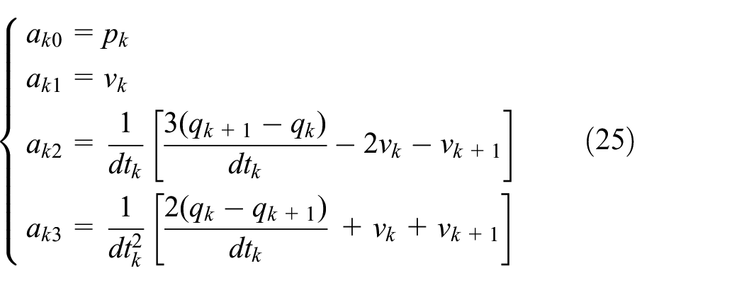
Trajectory parameter generation

By substituting p _k with the robot state quantities x _k , y _k , θ _k , ϕ _k in equation (25) respectively, and setting the initial and final linear velocity, angular velocity, and the steering wheel rotation angular velocity to 0, we can determine the coefficient of the way-point segments, a₀, a₁, a₂, a₃, b₀, b₁, b₂, b₃, c₀, c₁, c₂, c₃, d₀, d₁, d₂, d₃, recursively.

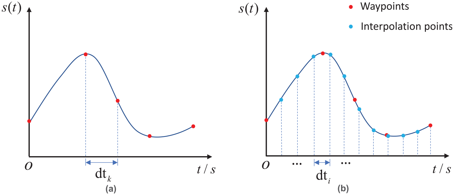
When the function of each trajectory is obtained, an interpolated smooth trajectory with equal time interval can be generated. In this work, the time interval for generating interpolation trajectory points is set to dt _i , as shown in Figure 9. Hence, the number of interpolated trajectory points is $n_i=\frac{t_n}{d{t}_i}$ , and t _i can be calculated according to the time interval of interpolation points dt _i as follows:

$$t_i=i\times d{t}_i,i=[1,n_i]$$

(26)

Figure 9.

State variable interpolation: (a) function of a certain state of way-points and (b) function of a certain state of interpolation points.

According to the timestamp t _i of each interpolation point and the corresponding s _k function, the state quantities x _i , y _i , θ _i , ϕ _i and control quantities v_{r_i}, w_{s_i} of the interpolation point can be obtained. Particularly, v_{r_i} is composed of the vertical and horizontal component velocities v_{x_i} and v_{y_i}, dependent on the interpolation point angle θ _i . The variable parameter of each interpolation point in the system can be determined using equations (27)–(29):

$$\begin{array}{c}\multicolumn{1}{c}{\left[\begin{array}{c}{x}_i\hfill \\ \multicolumn{1}{c}{y_i}\\ \multicolumn{1}{c}{{\theta }_i}\\ \multicolumn{1}{c}{{\varphi }_i}\end{array}\right]=[\begin{array}{cccc}{a}_{k0}\hfill & a_{k1}\hfill & a_{k2}\hfill & a_{k3}\hfill \\ \multicolumn{1}{c}{b_{k0}}& b_{k1}\hfill & b_{k2}\hfill & b_{k3}\hfill \\ \multicolumn{1}{c}{c_{k0}}& c_{k1}\hfill & c_{k2}\hfill & c_{k3}\hfill \\ \multicolumn{1}{c}{d_{k0}}& d_{k1}\hfill & d_{k2}\hfill & d_{k3}\hfill \end{array}]\left[\begin{array}{c}1\hfill \\ \multicolumn{1}{c}{d{t}_k}\\ \multicolumn{1}{c}{{\mathrm{dt}}_k^2}\\ \multicolumn{1}{c}{{\mathrm{dt}}_k^3}\end{array}\right]}\end{array}$$

(27)

$$\begin{array}{c}\multicolumn{1}{c}{\left[\begin{array}{c}{v}_{x\_i}\hfill \\ \multicolumn{1}{c}{v_{y\_i}}\\ \multicolumn{1}{c}{{\omega }_{\theta \_i}}\\ \multicolumn{1}{c}{{\omega }_{\varphi \_i}}\end{array}\right]=[\begin{array}{cccc}{a}_{k1}\hfill & 2a_{k2}\hfill & 3a_{k3}\hfill & 0\hfill \\ \multicolumn{1}{c}{b_{k1}}& 2b_{k2}\hfill & 3b_{k3}\hfill & 0\hfill \\ \multicolumn{1}{c}{c_{k1}}& 2c_{k2}\hfill & 3c_{k3}\hfill & 0\hfill \\ \multicolumn{1}{c}{d_{k1}}& 2d_{k2}\hfill & 3d_{k3}\hfill & 0\hfill \end{array}]\left[\begin{array}{c}1\hfill \\ \multicolumn{1}{c}{d{t}_k}\\ \multicolumn{1}{c}{{\mathrm{dt}}_k^2}\\ \multicolumn{1}{c}{{\mathrm{dt}}_k^3}\end{array}\right]}\end{array}$$

(28)

$$\begin{array}{c}\multicolumn{1}{c}{\left[\begin{array}{c}{a}_{x\_i}\hfill \\ \multicolumn{1}{c}{a_{y\_i}}\\ \multicolumn{1}{c}{{\alpha }_{\theta \_i}}\\ \multicolumn{1}{c}{{\alpha }_{\varphi \_i}}\end{array}\right]=[\begin{array}{cccc}2a_{k2}\hfill & 6a_{k3}\hfill & 0\hfill & 0\hfill \\ \multicolumn{1}{c}{2b_{k2}}& 6b_{k3}\hfill & 0\hfill & 0\hfill \\ \multicolumn{1}{c}{2c_{k2}}& 6c_{k3}\hfill & 0\hfill & 0\hfill \\ \multicolumn{1}{c}{2d_{k2}}& 6d_{k3}\hfill & 0\hfill & 0\hfill \end{array}]\left[\begin{array}{c}1\hfill \\ \multicolumn{1}{c}{d{t}_k}\\ \multicolumn{1}{c}{{\mathrm{dt}}_k^2}\\ \multicolumn{1}{c}{{\mathrm{dt}}_k^3}\end{array}\right]}\end{array}$$

(29)

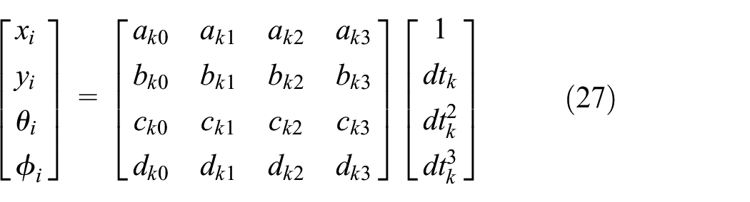
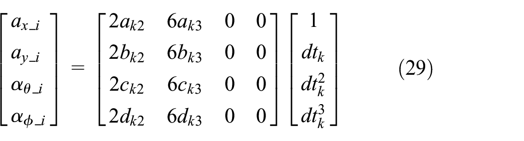
where a _k , b _k , c _k , d _k are the coefficient of the kth section. x _i , y _i , θ _i , ϕ _i are the states of each interpolation point, v_{x_i}, v_{y_i}, ω_{ϕ_i} are the control sequence quantities of each interpolation point. For better illustration, a arbitrary state quantity and its way-point interpolation diagram is shown in Figure 9.

The flow chart of the whole interpolation algorithm is further detailed in Algorithm 2, and its block diagram is shown in Figure 10. Inputs in Algorithm 2 include states of the path way-points x, y, θ, ϕ, number of way-points in the path n, starting velocity v₀, ending velocity v _n , and an array t for containing the timestamps of each waypoint t _i . Also, the user may choose to specify the time interval of interpolation points dt _i according to the actual situation. To calculate the velocity of each way-point, the algorithm proposed in this paper initializes a diagonally dominant matrix A and four column vectors c _x , c _y , c _θ , c _ϕ . Steps 2–11 in Algorithm 2 involve a recursive process to determine the values of the A, c _x , c _y , and c _ϕ matrix. Step 12 calculates the linear velocity, angular velocity, and steering wheel rotation angular velocity v _x , v _y , ω _θ , ω _ϕ of each way-point. Steps 14–18 calculate the way-point segment coefficient of cubic function (25). In steps 19–23, the parameters of each interpolation point is obtained in accordance to equation (27).

Algorithm 2.

Way-point smoothing interpolation algorithm.

Require: x, y, θ, ϕ, v0, vn, t, dti Ensure: Interpolated waypoints and velocities for x, y, θ, ϕ

1: Initialize matrix A and vectors cx, cy, cθ, cϕ

2: for k = 1 to n − 1 do

3:    $d{t}_k\leftarrow t(k+1)-t(k)$

4:    $d{t}_{k+1}\leftarrow t(k+2)-t(k+1)$

5:    $A[k,k-1]\leftarrow d{t}_{k+1}$

6:    $A[k,k]\leftarrow 2\times (d{t}_{k+1}+d{t}_k)$

7:    $A[k,k+1]\leftarrow d{t}_k$

8:    $\begin{array}{l}{c}_x[k,1]\leftarrow \frac{3}{d{t}_{k+1}\times d{t}_k}\times (d{t}_k^2\times (x(k+2)-x(k+1))\\ +d{t}_{k+1}^2\times (x(k+1)-x(k)))\end{array}$

9:    $\begin{array}{l}{c}_y[k,1]\leftarrow \frac{3}{d{t}_{k+1}\times d{t}_k}\times (d{t}_k^2\times (y(k+2)-y(k+1))\\ +d{t}_{k+1}^2\times (y(k+1)-y(k)))\end{array}$

10:    $\begin{array}{l}{c}_{\theta }[k,1]\leftarrow \frac{3}{d{t}_{k+1}\times d{t}_k}\times (d{t}_k^2\times (\theta (k+2)-\theta (k+1))\\ +d{t}_{k+1}^2\times (\theta (k+1)-\theta (k)))\end{array}$

11:    $\begin{array}{l}{c}_{\varphi }[k,1]\leftarrow \frac{3}{d{t}_{k+1}\times d{t}_k}\times (d{t}_k^2\times (\varphi (k+2)-\varphi (k+1))\\ +d{t}_{k+1}^2\times (\varphi (k+1)-\varphi (k)))\end{array}$

12: end for

13: v x , v y , v θ , v ϕ ← CalVelocity(A, c x , c y , c θ , c ϕ )

14: nt←t(1)

15: for k = 1 to n − 1 do

16:    $a_0(k),a_1(k),a_2(k),a_3(k)\leftarrow \mathrm{Decoupling}(x(k),v_x(k),t(k))$

17:    $b_0(k),b_1(k),b_2(k),b_3(k)\leftarrow \mathrm{Decoupling}(y(k),v_y(k),t(k))$

18:    $c_0(k),c_1(k),c_2(k),c_3(k)\leftarrow \mathrm{Decoupling}(\theta (k),v_{\theta }(k),t(k))$

19:    $d_0(k),d_1(k),d_2(k),d_3(k)\leftarrow \mathrm{Decoupling}(\varphi (k),v_{\varphi }(k),t(k))$

20:   while nt<t(k+1) do

21:     $x_i,v_{\mathrm{xi}},a_{\mathrm{xi}}\leftarrow \mathrm{CubicEquation}(a_0(k),a_1(k),a_2(k),a_3(k),\mathrm{nt})$

22:     $y_i,v_{\mathrm{yi}},a_{\mathrm{yi}}\leftarrow \mathrm{CubicEquation}(b_0(k),b_1(k),b_2(k),b_3(k),\mathrm{nt})$

23:     ${\theta }_i,{\omega }_{\theta i},{\alpha }_{\mathrm{xi}}\leftarrow \mathrm{CubicEquation}(c_0(k),c_1(k),c_2(k),c_3(k),\mathrm{nt})$

24:     ${\varphi }_i,{\omega }_{\mathrm{xi}},{\alpha }_{\mathrm{xi}}\leftarrow \mathrm{CubicEquation}(d_0(k),d_1(k),d_2(k),d_3(k),\mathrm{nt})$

25:     $\mathrm{nt}\leftarrow \mathrm{nt}+d{t}_i$

26:     $i\leftarrow i+1$

27:   End while

28: end for

Figure 10.

Algorithm 2 block diagram.

Trajectory rolling generation satisfying task completion time constraint

When the robot’s safety mechanism is triggered during navigation, reaching the target point according to the task time constraint necessitates trajectory regeneration of the remaining path according to the constraint conditions. If the actual needed time for the remaining navigation task exceeds the initial required task time, constraint fails. Here, the robot will endeavor to reach the target point as quickly as possible. Otherwise, the control instructions of the remaining paths will be recalculated according to the method proposed by section “Time allocation based on task-time constraints.” The regeneration flow chart is shown in Figure 11.

Figure 11.

Trajectory rolling generation.

When the safety trigger is released, the navigation system will recalculate the timestamp and control sequence quantities of each way-point in the remaining path to complete the task within the specified time. Assuming the safety stop occurred at the $n_p$ way-point, the driving time before the stop was $t_{\mathrm{drive}}$ , the stop wait time was $t_{\mathrm{stop}}$ , and the remaining time for the task was $t_{\mathrm{rest}}=t_{\mathrm{task}}-t_{\mathrm{stop}}-t_{\mathrm{drive}}$ , the shortest time $t_r$ for the remaining path would be calculated according to equation (30).

$$t_r=\sum _{k=n_p}^{n-1}d{t}_k$$

(30)

By comparing the shortest remaining path time t _r with the remaining task time t _rest , we evaluate the satisfaction of the task arrival time constraint. If t _r  > t _rest , it means that the robot cannot reach the target point within the given task time constraint. At this time, the robot is constrained to drive at the maximum velocity to reach the target point as soon as possible, and its time is t _task  = t _stop  + t _r . Otherwise, the time of the remaining path is recalculated.

As shown in Figure 12, task A is a trajectory generated according to a given time by the method proposed in section “Time allocation based on task-time constraints,” and the running time of the robot on this trajectory is the same, but in task B, the robot encountered an obstacle while driving and stopped suddenly for a while. Therefore, based on the time constraint t _rest for the remaining path, the time interval for the remaining path way-point segment can be derived using equation (31).

$$d{t}_{\mathrm{newtask}\_k}=\frac{t_{\mathrm{rest}}}{t_r}d{t}_k,k=n_p,\dots ,n-1$$

(31)

Figure 12.

Schematic diagram of way-point trajectory rolling generation.

Figure 13(a) shows a normal travel trajectory with no stopping from the start and end way-point (p₀ and p _n ). In Figure 13(b), p_{s_0} and p_{s_1} are the way-point before and after the emergency stop whereas the dashed yellow line represents the trajectory rolling generation of the remaining path time. p_{s_2} is the way-point after the emergency stop in Figure 13(c) and the red dashed line indicates that the robot is to travel to the end way-point in the shortest time to satisfy the constraints.

Figure 13.

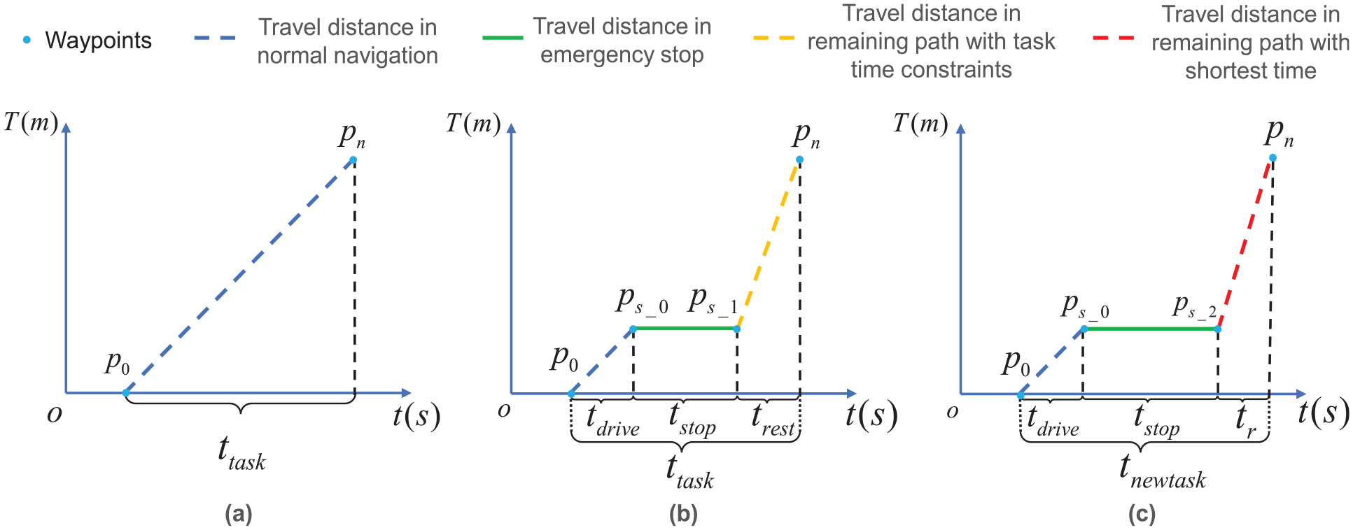
Travel distance of robot navigation: (a) Normal Navigation without Interruption, (b) Replanned Path after Emergency Stop with Sufficient Time Margin, (c) Replanned Path after Emergency Stop under Tight Task Time Constraint.

The control quantities for the way-points of the remaining paths are:

$$\begin{array}{c}{v}_{r\_\mathrm{newtask}\_k}=\frac{\sqrt{{(x_{k+1}-x_k)}^2-{(y_{k+1}-y_k)}^2}}{d{t}_{\mathrm{newtask}}}\hfill \\ {\omega }_{s\_\mathrm{newtask}\_k}=\frac{\sqrt{{({\theta }_{k+1}-{\theta }_k)}^2}}{d{t}_{\mathrm{newtask}}},k=n_p,\dots ,n-1\hfill \end{array}$$

(32)

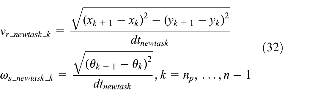
The robot trajectory rolling generation algorithm is shown in Algorithm 3. During robot navigation, the remaining path will be generated in real-time if the safety laser is triggered. Inputs of algorithm 3 consists of the drive time t _drive before robot emergency stop, emergency stop waiting time t _stop , target task time t _task , current way-point of the emergency stop n _p , the remaining number of way-points N, control commands v_{x_k}, v_{y_k}, v_{ϕ_k}, and the waypoint time interval sequence dt _k .

Algorithm 3.

Trajectory rolling generation algorithm.

Require: vx_k, vy_k, ωø_k, N, dtk, tstop, tdrive, ttask, np Ensure: Updated velocities vx_newwork_k, vy_newwork_k, ωϕ_newwork_k for k∈ [1, N]

1: if Alarm() then

2:   $t_{\mathrm{rest}}\leftarrow \mathrm{CalTime}(t_{\mathrm{stop}},t_{\mathrm{task}},t_{\mathrm{drive}},n_p)$

3:   $t_r\leftarrow \mathrm{CalTime}(n_p)$

4:  if $t_r>t_{\mathrm{rest}}$ then

5:     $t_{\mathrm{task}}\leftarrow t_{\mathrm{drive}}+t_{\mathrm{stop}}+t_r$

6:     $\mathrm{factor}\leftarrow 1$

7:  else

8:     $\mathrm{factor}\leftarrow \mathrm{Cal}\mathrm{Pr}\mathrm{oportional}(t_{\mathrm{rest}},t_r)$

9:  end if

10:  for k=1 to N do

11:     $d{t}_{\mathrm{newtask}}\leftarrow \mathrm{CalIntervalTime}(\mathrm{factor},d{t}_k)$

12:     $v_{x\_\mathrm{newwork}\_k}\leftarrow v_{x\_k}\times \mathrm{factor}$

13:     $v_{y\_\mathrm{newwork}\_k}\leftarrow v_{y\_k}\times \mathrm{factor}$

14:     $v_{\varphi \_\mathrm{newwork}\_k}\leftarrow v_{\varphi \_k}\times \mathrm{factor}$

end for

6:  end if

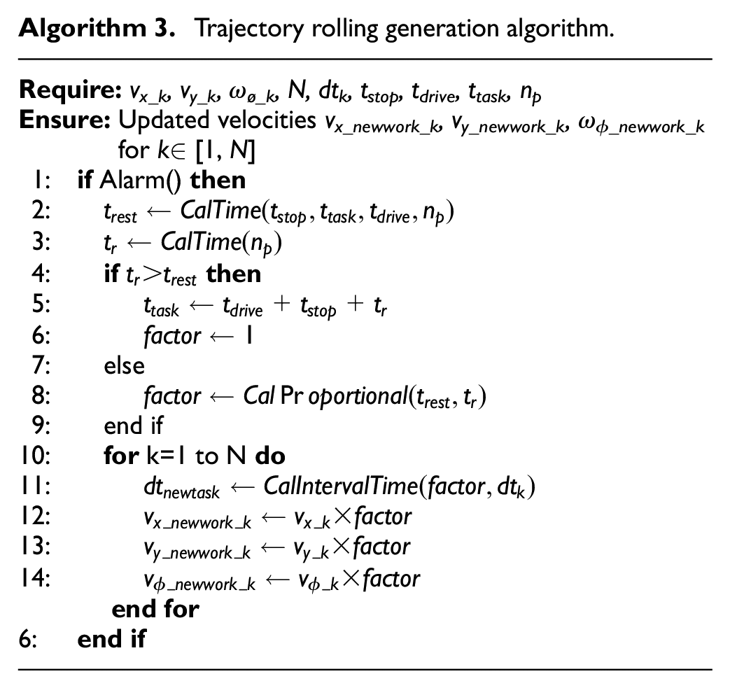
In step 1, judgment is made on whether the safety laser is triggered. The control instructions of the remaining path is planned when it is triggered, and the time of the remaining path of the task is calculated at t _rest . Step 2 and 3 calculates the shortest time of the remaining path t _r , corresponding to equation (30). Furthermore, steps 4–8 calculates the scale factor factor according to the relationship between the shortest time of the remaining path t _r and the actual remaining time t _rest . Finally, in steps 10–15, the control quantities of the remaining paths are set according to factor to realize the rolling generation of way-point timestamps.

Experiment and results

The algorithm proposed in this paper has been implemented in the robot operating system (ROS) framework for the evaluation of its comprehensive performance. For the evaluation, a PC with the ubuntu 16.04 OS, CPU model of i5-6200u, 8GB RAM, and 512GB of the hard disk was used. The factory simulation environment and forklift model satisfying car-like kinematics was developed using the gazebo software.^32–34 As the algorithm verification work was conducted in a simulated environment, the vehicle’s motion characteristics were ideal, meaning that whether or not the forklift was loaded, its motion characteristics were not affected. Obviously, in real-world, the load will have a corresponding impact on the motion characteristics of the forklift. If the load is heavy, a deviation of the forklift controller from the trajectory tracking will exist. In this experiment, the forklift was equipped with a high-precision positioning sensor with a translation and rotation positioning accuracy of 1 cm and 0.0012 radian, respectively. ³⁵ The forklift navigation control system could access the encoder and positioning data. As shown in Figure 14.

Figure 14.

Gazebo simulates environment: (a) factory environment in gazebo and (b) robot model in gazebo.

The forklift truck was equipped with two onboard lasers, among which the 2d safety laser sensor was located at the bottom of the forklift truck and was used to trigger the emergency mechanism for safety stop. The second, a 16-line 3D laser rangefinder with a viewing angle of 360°, was used for navigation, positioning, and safe obstacle avoidance. Also, a depth camera was installed at the vehicle’s rear, and was used to obtain pallet identification data. Figure 15, shows (a) A 2D grid map of the factory simulation environment, (b) The front of the forklift, and (c) The back of the forklift.

Figure 15.

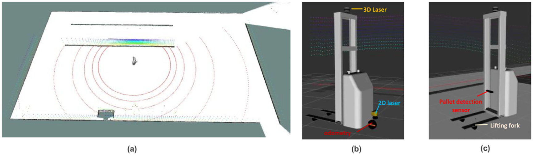
2d grid map and robot model: (a) 2d grid map, (b) forklift robot back view, and (c) forklift robot front view.

Calculation of way-point timestamp with minimum task time

To provide a comprehensive explanation of the trajectory generation algorithm proposed in this paper, the specific method adopted by the path planning module and its detailed process are outlined below: First, the navigation area and obstacle locations are defined based on the Voronoi State Lattice map. Next, the ARA* (Anytime Repairing A*) planner is employed to search for the optimal path on the state grid map, ensuring the path is collision-free and adheres to the vehicle’s kinematic constraints. Subsequently, safe boundaries are extracted from the planned path to define lateral and longitudinal safety constraints for the path waypoints, ensuring safety during the path optimization and smoothing processes. Path smoothing further optimizes the original waypoints to generate a smooth path that complies with the vehicle’s kinematic and dynamic constraints. Finally, the path generation module outputs a sequence of smooth waypoints containing the state variables (x _i , y _i , θ _i , ϕ _i ). The smooth way-point is shown in Figure 16. When the system inputs the path, it will calculate the shortest time between way-points according to the kinematics and dynamics constraints, and get the timestamp information of each way-point.

Figure 16.

Way-points of smooth path.

Experimental evaluation values are set as follows, the maximum linear velocity v_max = 1 m/s, the maximum linear acceleration a_max = 1 m/s², the maximum steering wheel rotation angular velocity w _s  = 1 rad/s, and the maximum angular velocity w _r  = 1 rad/s. The maximum velocity and acceleration constraints were chosen based on the characteristics of the forklift and typical working requirements in the factory setting. Specifically, the values were selected to satisfy the maximum acceleration constraint while ensuring that the forklift can safely navigate in the factory environment. The information on the state quantity and timestamp change of each waypoint generated by the method proposed in this paper is shown in Figure 17. According to the experimental data, the minimum navigation task time is 34 s under vehicle kinematics and dynamics constraints.

Figure 17.

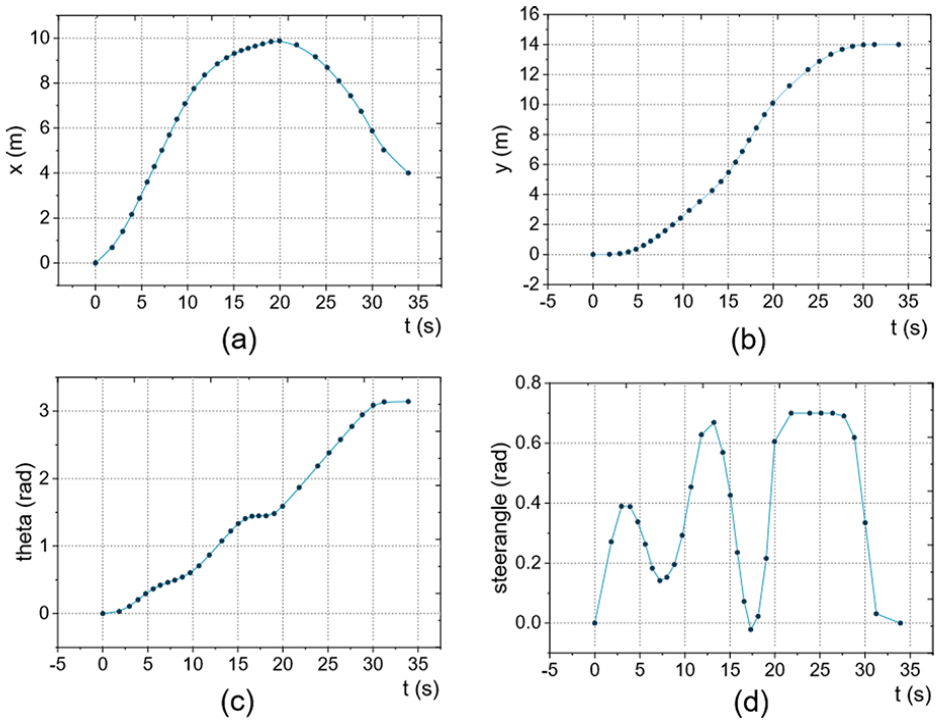
Calculation of way-point timestamp with the least task time: (a) time-varying image of way-point state of x, (b) time-varying image of way-point state of y, (c) time-varying image of way-point state of theta, and (d) time-varying image of waypoint state of steering angle.

Calculation of way-point timestamp with different task time constraints

In this experiment, two different target task time constraints of 50 and 70 s are set, respectively, and the timestamp information of way-points corresponding to different task times is calculated according to the algorithm 3 presented in this paper. The trajectory generation that satisfies the task time constraint when the forklift performs navigation tasks is independent of whether the forklift is loaded or not. When the obstacle avoidance module detects a dynamic obstacle, the robot will come to an emergency stop until it has passed.

The experimental results are shown in Figure 18, and the timestamp information of robot way-points corresponding to different target times are generated, respectively. Among them, the blue dots represent the state quantity and timestamp information that meet the minimum time of robot kinematics and dynamics. The red dot represents the way-point timestamp information obtained by the trajectory generation algorithm 3 proposed in this paper when the target task time is the 50 s. The green dot represents the timestamp information of the way-point when the target task time is in the 70 s.

Figure 18.

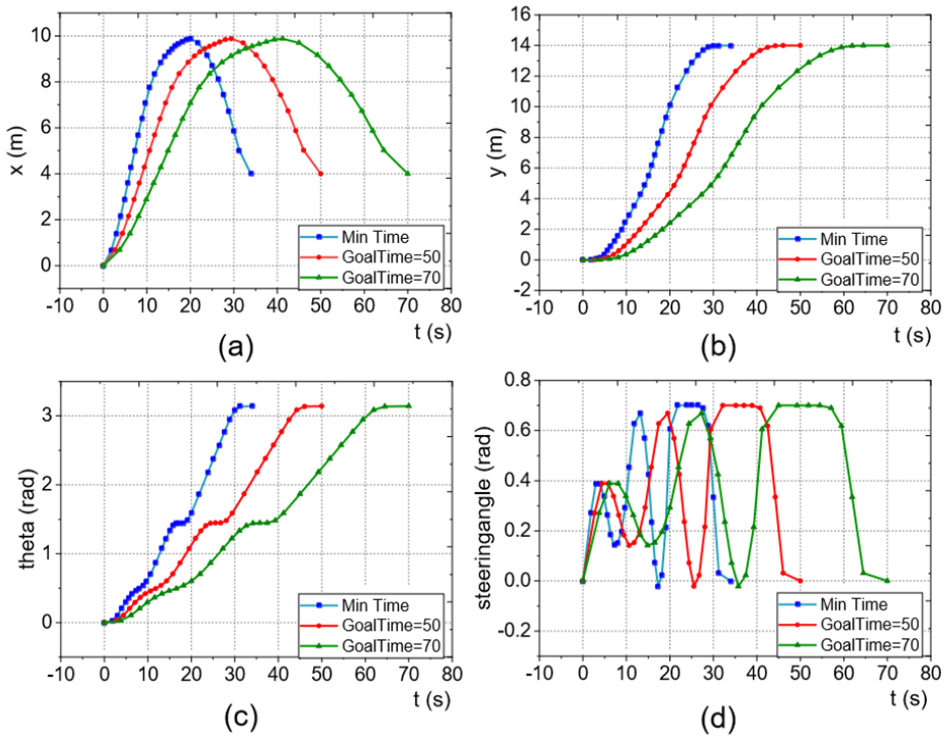
Timestamp calculation of waypoint with different task time constraints: (a) comparison diagram of x, (b) comparison diagram of y, (c) comparison diagram of theta, and (d) comparison diagram of steering angle.

From the analysis of the experimental results, it can be concluded that when the task target time constraints are set to 50 and 70 s, the timestamps of each way-point in the trajectory changed proportionally. Therefore, the requirements of trajectory generation with different task time constraints is satisfied.

Comparative experiment of different trajectory interpolation methods

In order to verify the effect of using a non-interpolation algorithm between way-points, different methods are used to interpolate way-points in the same path. We compare the cubic spline interpolation with cubic polynomial, quintic polynomial, and bezier curve interpolation methods used in this paper.

When cubic polynomial interpolation was used, the input data were the state and velocity of each way-point on the trajectory. However, because the influence of acceleration was not considered, the acceleration was discontinuous (not smooth). The acceleration change rate was significant, which led to the collision or unpredictable vibration of the robot, resulting in safety hazards.

When using quintic polynomial interpolation, the input data were the way-point’s state, velocity, and acceleration on the trajectory. Although the quintic polynomial interpolation method can ensure the continuity and smoothness of acceleration, it cannot set the maximum acceleration threshold. At the same time, due to the use of uniform nodes to construct high-order polynomial interpolation, the Runge phenomenon can occur, which leads to the deviation of interpolation results from the original function, and inability to constrain acceleration to a small range.

Subsequently, when cubic spline interpolation was used, the input data were the state variables and endpoint velocity values of each way-point on the path. The equation coefficients between way-points were solved by adding the conditions of continuous velocity and acceleration of way-points. The velocity obtained by this method was not abrupt but smooth, and the trajectory satisfied the constraints of maximum velocity and maximum acceleration.

We further compared cubic spline interpolation with cubic polynomial interpolation, quintic polynomial interpolation, and bezier curve interpolation. When interpolating, the system smooths the start and stop segments and, sets the velocity at the starting and ending points to 0. The experimental results are shown in Figures 19 to 21. Figure 19 presents the state quantities of the way-points for each interpolation method, showing that the state values of all four methods are almost coincident, indicating they all meet the position fitting accuracy requirement.

Figure 19.

Comparison of different curve interpolation methods (states): (a) x-coordinate, (b) y-coordinate, (c) heading angle θ, and (d) steering angle ϕ.

Figure 20.

Comparison of different curve interpolation methods (velocity): (a) x-axis velocity, (b) y-axis velocity, (c) heading angular velocity, and (d) steering angular velocity.

Figure 21.

Comparison of different curve interpolation methods (acceleration): (a) x-axis acceleration, (b) y-axis acceleration, (c) heading angular acceleration, and (d) steering angular acceleration.

Figure 20 shows the velocity curves of the way-points, where all methods achieve continuous velocity transitions. Both cubic spline and quintic polynomial methods provide smooth velocity curves. Bezier interpolation also achieves a smooth velocity profile, although slight oscillations are observed near segments with sharp transitions. In contrast, the velocity curve obtained by the cubic polynomial interpolation method is continuous but not smooth, failing to meet the requirements of smooth control inputs.

Figure 21 illustrates the acceleration curves of the way-points. The acceleration curve obtained by the cubic polynomial interpolation method is discontinuous, causing oscillations in motor control inputs. Quintic polynomial interpolation ensures continuous and smooth acceleration but suffers from the Runge phenomenon, which can exceed the vehicle’s maximum acceleration constraint. The cubic spline interpolation method produces a continuous acceleration curve that satisfies the vehicle’s maximum acceleration constraint. Bezier interpolation also provides continuous acceleration; however, in sharp turn regions, local spikes in acceleration are observed, occasionally exceeding dynamic constraints due to the sensitivity of Bezier curves to control point distribution.

Based on the results of this study (see Table 1), the TTRP method demonstrates significant advantages over cubic polynomial, quintic polynomial, and Bezier interpolation in terms of trajectory smoothness, stability, and energy efficiency. Specifically, the TTRP method reduces the maximum speed variation by 58.5%, 61.0%, and 61.4% compared to cubic, quintic, and Bezier interpolation, respectively, indicating its ability to minimize abrupt speed changes, thereby enhancing trajectory smoothness and control stability. Furthermore, the TTRP method lowers the maximum jerk by 94.7%, 89.7%, and 15.5% compared to cubic, quintic, and Bezier interpolation, respectively, illustrating its exceptional capability to reduce sudden acceleration changes. This reduction mitigates mechanical shocks and enhances trajectory-following stability. Similarly, in terms of the standard deviation of acceleration rate, the TTRP method achieves reductions of 90.9%, 88.1%, and 13.7% compared to cubic, quintic, and Bezier interpolation, respectively, emphasizing its capacity to maintain consistent acceleration throughout the trajectory and reduce motion fluctuations. These findings demonstrate that the TTRP method is a superior choice for high-precision robotic trajectory tracking, significantly improving smoothness, stability, and safety, while also minimizing energy consumption and mechanical impact on the system.

Table 1.

Comprehensive performance comparison of trajectory interpolation methods for robotic motion.

Metric	Component	TTRP	Cubic polynomial	Quintic polynomial	Bezier	TTRP vs cubic (%)	TTRP vs quintic (%)	TTRP vs Bezier (%)
Maximum speed change rate (m/s2)	x Direction	0.5968	0.9203	0.9607	1.1603	35.15	37.88	48.57
	y Direction	0.1982	0.8270	0.9012	0.8553	76.03	78.01	76.83
	θ Direction	0.1129	0.3275	0.3429	0.3809	65.53	67.2	70.36
	ø Direction	0.4965	1.4689	1.5694	1.4762	66.20	68.3	66.37
	Overall	0.8091	1.949	2.078	2.097	58.5	61.0	61.4
Maximum jerk (m/s3)	x Direction	0.3055	11.8842	4.4527	0.754	97.43	93.14	59.48
	y Direction	0.2413	9.6626	5.5682	0.540	97.50	95.67	55.29
	θ Direction	0.1052	3.8902	1.8398	0.198	97.30	94.28	46.87
	ϕ Direction	1.0489	15.2075	7.9012	0.933	93.10	86.8	−12.39
	Overall	1.1238	21.91	10.81	1.33	94.7	89.7	15.5
Standard deviation of acceleration rate (m/s3)	x Direction	0.0743	1.0213	0.6896	0.138	92.72	89.23	46.14
	y Direction	0.0455	0.9858	0.7835	0.105	95.38	94.19	56.67
	θ Direction	0.0242	0.4707	0.3460	0.041	94.86	93.01	40.98
	ϕ Direction	0.1760	1.5662	1.2615	0.145	88.76	86.05	−21.38
	Overall	0.1977	2.165	1.673	0.229	90.9	88.1	13.7

Evaluating trajectory interpolation and tracking performance

To comprehensively evaluate the performance of different trajectory interpolation methods, this experiment assesses their effectiveness in trajectory tracking. A total of 30 randomly generated irregular trajectories were used as test cases, encompassing sharp turns, curves, and complex path shapes. These trajectories were interpolated using four methods: TTRP (based on cubic spline interpolation), cubic polynomial interpolation, quintic polynomial interpolation, and Bezier curve interpolation. The interpolated trajectories were used as the desired paths, and a unified MPC ³⁶ trajectory tracking control algorithm was employed to analyze the performance of each interpolation method in terms of tracking error, smoothness, and computational time.

In this experiment, we designed the experimental scenario as shown in Figure 22. The scenario includes a starting region and a target region, marked with dashed lines, between which 30 trajectories were randomly generated. The generated trajectories encompass various types, such as polylines with sharp turns, irregular curves, and rapidly converging spiral paths, to comprehensively simulate the complex task requirements of real-world environments. These trajectories cover diverse combinations of starting and target poses, ensuring the comprehensiveness and representativeness of the experiment. Subsequently, for each trajectory, four different interpolation methods were applied to generate the desired trajectory, and a uniformly configured Model Predictive Control (MPC) algorithm was used for trajectory tracking. This setup enables a comprehensive evaluation of the tracking accuracy, smoothness, and stability of the algorithms, providing a reliable basis for performance analysis.

Figure 22.

Test environment with randomly selected positions making up 30 trajectory paths.

To comprehensively evaluate the performance of different trajectory interpolation methods in trajectory tracking tasks for single-steering-wheel forklifts, the following key metrics were selected: tracking error, smoothness, control energy consumption, and computational efficiency. The tracking error is quantified using the Root Mean Square Error (RMSE) of the position error and heading angle error, which respectively measure the spatial deviation and directional deviation of the vehicle during trajectory tracking. The position error is defined as:

$${\mathrm{RMSE}}_{POS}=\sqrt{\frac{1}{N}\sum _{i=1}^N({(x_i^{desired}-x_i^{actual})}^2+{(y_i^{desired}-y_i^{actual})}^2)}$$

(33)

The heading angle error is defined as:

$${\mathrm{RMSE}}_{POS}=\sqrt{\frac{1}{N}\sum _{i=1}^N{({\theta }_i^{desired}-{\theta }_i^{actual})}^2}$$

(34)

Here, N represents the number of sampled points, ( $x_i^{\mathrm{desired}}$ , $y_i^{\mathrm{desired}}$ , θ _i ^desired) denotes the coordinates and heading angle of the desired trajectory, and ( $x_i^{\mathrm{desired}}$ , θ _i ^actual) represents the coordinates and heading angle of the actual trajectory. Additionally, to evaluate the smoothness and stability of the trajectory, the maximum rate of change in velocity (m/s²) and maximum jerk (m/s³) are used as indicators. The maximum rate of change in velocity measures the degree of speed fluctuations in the trajectory, while the maximum jerk reflects the severity of abrupt accelerations in the trajectory. The trajectory interpolation computation time (in milliseconds) is employed as a metric to evaluate the computational efficiency of the algorithm, reflecting its real-time performance. These indicators comprehensively and scientifically quantify the performance of interpolation methods across three aspects: tracking accuracy, motion stability, and real-time efficiency. They provide a clear basis for the comparative analysis of experimental results.

The experimental results are summarized in Table 2, where the TTRP method demonstrates superior performance across key metrics, including tracking error, smoothness, and computational efficiency. Specifically, the average position error (RMSE_pos) for TTRP is 0.0184 m, which is significantly lower than that of cubic polynomial interpolation (0.0338 m), quintic polynomial interpolation (0.0262 m), and Bezier curve interpolation (0.0237 m). In terms of heading angle error (RMSE_angle), TTRP achieves an error of 0.0137 rad, which is also notably better than the other methods.

Table 2.

Performance comparison of trajectory tracking for single-steering-wheel forklift.

Metric	TTRP	Cubic polynomial	Quintic polynomial	Bezier curve
RMSEpos (m)	0.0184	0.0338	0.0262	0.0237
RMSEangle (rad)	0.0137	0.0287	0.0235	0.0176
Max acceleration (m/s2)	0.6123	1.4527	1.1234	1.2845
Max jerk (m/s3)	1.2985	6.7385	4.5273	2.4537
Interpolation time (ms)	13.7	12.3	17.4	19.8

Additionally, the maximum rate of change in velocity and maximum jerk for the TTRP method are 0.6123 m/s² and 1.2985 m/s³, respectively, demonstrating exceptional smoothness of the trajectory. In contrast, the smoothness of other methods is inferior, with cubic polynomial interpolation exhibiting significant oscillations. Although the cubic polynomial interpolation method has the shortest computation time (12.3 ms), its performance is insufficient to support high-precision tasks. In comparison, the TTRP method achieves outstanding overall performance within a computation time of 13.7 ms, demonstrating excellent real-time capability.

Figure 23 presents a comparison of the tracking errors for TTRP, Cubic Polynomial, Quintic Polynomial, and Bezier curve interpolation methods under MPC tracking. The results demonstrate that the TTRP method exhibits significant advantages in tracking accuracy for the X direction, Y direction, and heading angle (θ). For the X direction, the TTRP method achieves the lowest median error and the smallest error range, indicating precise and stable trajectory tracking, whereas the Cubic Polynomial method shows the widest error range and the largest fluctuations. For the Y direction, TTRP also achieves the lowest median error and the narrowest range of distribution. In contrast, the Cubic Polynomial and Quintic Polynomial methods exhibit higher errors with greater instability, while the Bezier curve interpolation method shows some improvement but still lags behind TTRP. In terms of the heading angle (θ), the TTRP method achieves the smallest error with the most compact distribution, highlighting superior directional control accuracy and stability, whereas the Cubic Polynomial method has the widest error range, indicating lower directional tracking precision. Overall, the TTRP method consistently outperforms the other interpolation methods in all three dimensions, demonstrating higher accuracy and smaller error fluctuations, making it a robust approach for trajectory tracking under time-constrained tasks and dynamic environments.

Figure 23.

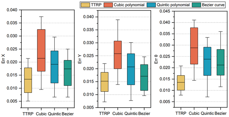
Box plot comparison of tracking errors for different trajectory interpolation methods using MPC.

The experimental results validate the significant advantages of the TTRP method in trajectory tracking for single-steering-wheel forklifts, demonstrating its ability to achieve high-precision and high-smoothness trajectory tracking with relatively low computational cost. Furthermore, the experiments reveal the limitations of other interpolation methods. For instance, while cubic polynomial interpolation offers higher computational efficiency, it suffers from larger tracking errors and higher energy consumption. Quintic polynomial interpolation shows insufficient adaptability to sharp changes, and Bezier curves exhibit instability due to their sensitivity to the distribution of control points, posing additional challenges for complex trajectories. Overall, the TTRP method is well-suited for high-precision robotic motion control tasks in dynamic and complex environments.

Trajectory rolling generation with different safety stop wait time

To test the extent to which the rolling trajectory generation method satisfy the requirements of the task execution time constraint under triggered safety obstacle avoidance condition, the robot’s safety stop is to be triggered in the middle of a simulated task execution. Different wait duration after stoppage were set to verify the effectiveness of the rolling trajectory generation algorithm.

During the experiment, the execution time of the navigation task was set to 50 s, and the robot generates the original trajectory according to the proposed method. When the robot moved for about 14.3 s, the safety laser was triggered, and the robot stopped for 3, 5, and 10 s, respectively. The simulation is shown in Figure 24.

Figure 24.

In the simulation environment, the forklift encountered an obstacle at 14.3 s and stopped halfway: (a) 2D environment map and (b) 3D Gazebo environment.

For the robot wait time of 3 s after stopping, it can be seen from Figures 25, 26 and Table 3 that the robot generates the trajectory according to the target time after driving for 14.3 s. When the robot stops, the shortest time of the remaining path was calculated to be 26.4 s, while the stop timestamp was 14.3 s. When the robot starts to move again, the remaining time according to the rolling generation algorithm was calculated to be 32.7 s.

Figure 25.

Trajectory rolling generation state values at different safety braking timestamps: (a) x-state before and after safety trigger, (b) y-state before and after safety trigger, (c) heading angle (θ) before and after safety trigger, and (d) steering angle (ϕ) before and after safety trigger.

Figure 26.

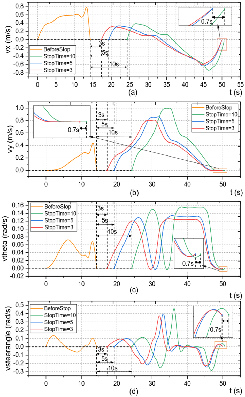
Trajectory rolling generation velocities at different safety braking times: (a) x-velocity before and after safety trigger, (b) y-velocity before and after safety trigger, (c) heading angular velocity (θ) before and after safety trigger, and (d) steering angular velocity (ϕ) before and after safety trigger.

Table 3.

Trajectory rolling generation at different parking times.

Path	Task time (s)	Time before stopping (s)	Stopping time (s)	STTP (s)	RTTTS (s)	RRTTS (s)	Total time (s)	WAD
Path1 (red)	50	14.3	3	26.4	32.7	32.7	50	Yes
Path2 (blue)	50	14.3	5	26.4	30.7	30.7	50	Yes
Path3 (green)	50	14.3	10	26.4	25.7	26.4	50.7	No

STTS: shortest time of the trajectory after stopping (s); RTTTS: rest task time of the trajectory after stopping (s); RRTTS: rest real time of the trajectory after stopping (s); WAD: whether to arrive at the destination according to the task time.

Because the remaining time of the task was longer than the shortest time of the remaining path, the robot could generate the path according to the remaining time.

When the robot stops for 5 s, the trajectory of the first 14.3 s was generated in the same way as before. The timestamp when stopping was 14.3 s. When the robot starts moving again, the remaining time was calculated to be 30.7 s. Similarly, the remaining time of the task was longer than the shortest time of the remaining path, and the robot could generate the path according to the remaining time.

When the robot stops for 10 s, the remaining time of the task was only 25.7 s, which is less than the shortest time of the remaining path, 26.4 s. Therefore, the robot tried to reach the target point faster under its kinematic constraints. At this time, the task time is the sum of the time before stopping, including the stopping time and the shortest time of the remaining path. Finally, the robot reached the task finishing point with a total task time of 50.7 s.

The experimental results show that the trajectory rolling generation method based on task completion time constraint proposed in this paper is effective.

Conclusions

In this paper, we propose a robot trajectory rolling generation algorithm based on task completion time constraints. This algorithm decouples the trajectory rolling generation problem into time planning for path way-points and smooth interpolation between way-points by calculating control commands and timestamps for each path point, ensuring that the robot completes tasks on time. In particular, the algorithm is capable of replanning the control commands and time intervals for each path point based on given user task-time duration, offering a new solution for robot task planning and replanning, especially suited for dynamic environments and emergency safety shutdowns. Experimental results demonstrate that the proposed algorithm effectively regenerates trajectories that meet kinematic and dynamic requirements after an emergency shutdown, while satisfying the preset task execution time constraints.

Moreover, the versatility of the TTRP algorithm makes it applicable to serial, parallel, and hybrid robots. For serial robots, Toz and Kucuk ³⁷ highlighted the computational efficiency characteristics of fundamental serial robot kinematics. The TTRP algorithm, with its timestamp calculation and trajectory interpolation framework, is highly compatible with the kinematic models of serial robots. For parallel robots, studies by Toz and Kucuk^38,39 and Inner and Kucuk ⁴⁰ demonstrated that the complex inverse kinematics and dynamic constraints of multi-degree-of-freedom systems demand greater flexibility. The TTRP algorithm can accommodate these requirements by integrating inverse kinematics solutions, ensuring that timestamp calculations and trajectory planning respect the constraints of parallel robots. Hybrid robots combine the characteristics of serial and parallel mechanisms, presenting unique challenges. The study by Kucuk ⁴¹ provided theoretical support for solving the kinematics of hybrid robots. By optimizing trajectory generation and incorporating constraints, the TTRP algorithm can effectively address these challenges, enabling smooth and feasible trajectory planning for hybrid robots.

In conclusion, the TTRP algorithm proposed in this paper is a universal trajectory planning framework, and its core ideas can be applied to various types of robotic models, such as wheeled robots in warehouses, drones, and various robotic arms. The algorithm is highly versatile, allowing for adjustments based on the physical characteristics and operational requirements of the target robot, making it widely applicable across different robotic platforms. Future research will further address the issue of ensuring smooth connections in the trajectories generated by the rolling method before and after emergency shutdowns, enhancing the stability of robot movement in complex environments. Additionally, we will continue to explore the impact of load on speed constraints to improve its effectiveness and robustness in practical applications.