Calculation parameter correction of steel truss nodal plate based on machine learning theory

Abstract

To improve the accuracy of deformation calculations in the finite element modeling of steel trusses, a method is proposed to modify the rigid arm by accounting for the stiffness of the nodal plate. A digital twin is established for each control parameter of the nodal plate, and the rigid arm lengths are adjusted to achieve displacement matching with a high-precision plate element model. A Bayesian decision tree and an artificial neural network (ANN) are then used to map the relationship between the twin parameters and the rigid arm length coefficients, respectively, to correct for stiffness. The reliability of these two machine learning methods was confirmed through mutual validation, with results showing that the ANN produced more accurate rigid arm length coefficients, while the Bayesian decision tree performed slightly less well. Both methods, however, successfully overcome the limitations of traditional beam elements, which do not account for nodal plate stiffness. Finally, large-scale bridge engineering examples using steel trusses demonstrate that correcting the rigid arm length significantly improves the calculation accuracy of commonly used beam elements. This approach also reduces the complexity of beam-plate coupling, making the modeling process more convenient, faster, and efficient.

Introduction

Currently, in the manufacture of large-span steel truss girder sections, the overall node plate technology is the preferred method. The thicker node plate is typically welded to the main chord, with the boundary for web connection cut out. This design rapidly increases the web thickness and width of all the rods in the node area, ensuring greater stiffness of the overall node. The integral node technology was first used in the construction of the Sunkou Yellow River Bridge in 1995, and with the widespread adoption of large-span highway-railway dual-purpose steel truss bridges, this fabrication technology has matured significantly. However, controlling the alignment of the main truss during construction remains a significant challenge, primarily due to the inaccurate stiffness calculation or the complexity of modeling integral nodes.

Huang et al. ¹ and Zhang et al. ² studied the effects of integral node stiffness on the displacement, stress, and vibration modes of steel trusses. Sheng et al. ³ found that integral node stiffness has the greatest impact on the secondary internal forces in vertical web bars. Tong and Ai ⁴ and Gao et al. ⁵ observed a consistent pattern in the deflection of steel trusses across different node stiffness models, with the rigid arm model producing the least deflection, followed by the rigid joint model, and finally the articulated model. Lu et al. ⁶ proposed a modified formula for calculating nodal stiffness, which takes into account nodal plate thickness, axial compression ratio, and weld temperature difference stress.

The studies mentioned above^1–6 are directly related to the stiffness of steel truss nodal plates, which, overall, is a relatively limited area of research. There are even fewer studies that apply machine learning to this field. Only in the works of Rahman et al. ⁷ and Li ⁸ are machine learning methods used to study other components of nodal plates. Rahman et al. ⁷ leveraged the interpretability of machine learning to predict the ultimate load-carrying capacity of nodal plates, while Li ⁸ developed a GA-BP neural network model to optimize nodal construction parameters in steel joist beams, aimed at reducing concentrated stresses in the nodes.

Li, ⁸ Hou, ⁹ and Shang ¹⁰ studied the force transmission characteristics of connection nodes under various conditions, such as under-torquing, over-torquing, and even bolt fractures in high-strength steel truss bolts. Liu and Sun ¹¹ conducted a nonlinear stress analysis on the integral nodes of steel truss bridges, revealing that most areas of the nodes operate within the elastic range, with only a few regions showing stress concentrations higher than those in the connected bars. The studies^8–11 focus on bridges with main spans of 200 m or less, and all of them employed overall beam element models. For local calculations, the isolators at the nodes were modeled using plate elements. Due to computational limitations, these small bridge models cannot fully implement plate element modeling for the entire structure. This challenge becomes even more pronounced in large-span steel truss bridges with main spans exceeding 500 m. As a result, beam element modeling remains the mainstream approach for overall modeling tasks in steel truss bridges, with refined plate elements introduced only in localized stress analyses.

Aside from the limited literature on steel truss bridges that focuses on the stiffness of nodal plates, most studies on steel nodes and nodal plates have explored other areas, especially in building structures, which are less relevant to this study. Zaharia and Dubina ¹² proposed and verified a formula for calculating node stiffness through single-node joint tests and full-scale truss experiments, using this theory to further calculate the flexural length of web bars. Song et al. ¹³ compared various design methods for steel truss nodal plates and evaluated Whitmore’s method, as well as block shear and buckling design methods. Liu et al. ¹⁴ conducted both experimental and numerical studies on the load-carrying capacity of K-type steel pipe nodal plates in transmission towers. Ling et al. ¹⁵ compiled a review of metal-plate-connected (MPC) wood joints, comparing the static and dynamic properties of wood structures based on various codes, loads, and MPC shapes. Wang et al. ¹⁶ experimented with glued laminated wood as a substitute for steel in testing the mechanical properties of steel truss nodal plates, with results that aligned with numerical calculations. Malgorzata et al. ¹⁷ investigated the load-carrying capacity of positively eccentric CFS standard trusses through experiments and numerical simulations, analyzing the connection damage mechanisms. Jiang et al. ¹⁸ experimented with scaled-down models of K-filled concrete truss nodes and derived equations for stress concentrations. Zou et al. ¹⁹ studied the performance of FRP nodal plates in terms of stiffness, strength, and fatigue. Lastly, Siekierski ²⁰ proposed a modified beam element model that addressed numerical anomalies caused by stress concentrations, improving the accuracy of stress calculations.

Machine learning algorithms are proficient at uncovering the relationships between features and labels, such as the study in this paper on the impact of design parameters of steel trusses on the stiffness of node plates. Research in other fields also follows a similar approach. For example, Rajender et al. ²¹ considered both direct factors (corrosion rate, rebar diameter, cover thickness) and indirect factors (the heterogeneous properties of concrete, the permeability of concrete, and the bond slip temperature of concrete) as independent variables in their study on predicting the lifespan of concrete. Machine learning effectively explained the relationship between these parameters and the concrete lifespan. Similarly, Zhu et al. ²² used material dispersion, load fluctuation, and geometrical tolerance as independent variables, and the support vector machine algorithm was able to easily capture the nonlinear response of turbine blades. Yang et al. ²³ focused on exploring the impact of learning functions on analytical engineering parameters, greatly improving the accuracy and efficiency of machine learning algorithms in evaluating engineering parameters.

A review of the literature shows that most studies do not focus heavily on the stiffness of steel truss nodal plates. In design practice and construction control, the finite element models of steel truss bridges often rely on simple beam element simulations, which ignore nodal plate stiffness and result in an overestimation of deflection. To mitigate this, several scholars^1–6 have proposed using a node rigid arm to reduce deflection. However, the rigid arm domain defined by the nodal plate contour is often too large, leading to an underestimation of deflection.

This paper proposes the introduction of a modified rigid arm to simulate the entire node and address these deficiencies. By setting appropriate values for the rigid arm’s length, the beam element model can achieve deflection accuracy comparable to that of a plate element model. However, traditional methods for correcting the stiffness of nodal plates remain somewhat limited and lack standardization. These methods often solve only isolated problems, which significantly reduces their general applicability – making them less suitable for the large-scale, standardized production and installation of steel trusses. In contrast to approaches that extract stiffness characteristics from individual steel truss projects, the machine learning method proposed in this paper leverages a large database of nodal plate dimensions. This allows for the consideration of various types of nodal plate stiffness, offering greater versatility and broader applicability.

Nodal plate parametric analysis method

Node plate digital twin library parameterization

The dimensions of the nodal plate are the most direct factors influencing node stiffness, and these parameters include the thickness of the nodal plate tk, the arc radius of the nodal plate r, the height of the chord section h1, and the height of the web section h2. Considering that node stiffness is also affected by the stiffness of the rods, the following additional parameters should be considered: the width of the rods w, the chord plate thicknesses (ht1, wt1), and the web thicknesses (ht2, wt2). Nodal plates and bars can be modeled as rigid connections, semi-rigid connections, or articulated connections. The depth of the web rod inserted into the nodal plate determines these boundary conditions, leading to the need for the insertion depth parameter dp to be set accordingly. All the parameters considered are shown in Figure 1.

Figure 1.

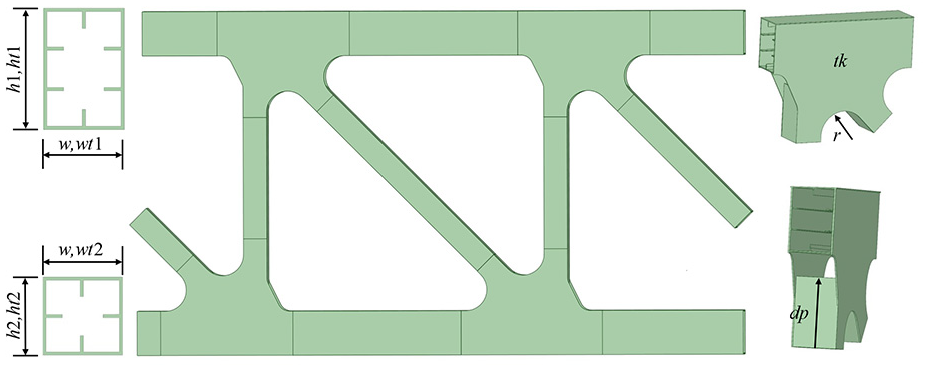
Parameterization of truss and node plate dimensions.

To ensure that the shape of the nodal plate meets the required parameters, control points A₁ to A₁₂ are set to achieve basic alignment between the element plate and the native plate. Additionally, to minimize the time and memory required for mesh division of the plate elements, the arc segments are represented by two straight-line sections instead of curves. This allows for the creation of larger plate elements, reducing the total number of elements in a single nodal plate to 16. Table 1 presents the geometric parameter control coordinates for the nodal plate, while Figure 2 illustrates the positions of the control points used to define the nodal plate shape.

Table 1.

Nodal plate geometry parameter control coordinates.

Control points	Coordinates
	$x$	$y$
$A_1$	$-h2$	$(h1)/2$
$A_2$	$-h2$	$-(h1)/2$
$A_3$	$-(h2)/2$	$-(h1)/2-h2$
$A_4$	$-(h2)/2$	$-((h2)/2+r)·\tan (67.5^{°})$
$A_5$	$(h2)/2$	$-((h2)/2+r)·\tan (67.5^{°})$
$A_6$	$r+(h2)/2-r·\cos (67.5^{°})$	$r·\sin (67.5^{°})-((h2)/2+r)·\tan (67.5^{°})$
$A_7$	$r+(h2)/2+r·\cos ({45}^{°})$	$r·\sin ({45}^{°})-((h2)/2+r)·\tan (67.5^{°})$
$A_8$	$A_{12}(x)-((h2)+r)·\cos ({45}^{°})$	$-(h1)/2-r-(r+h2)·\cos ({45}^{°})$
$A_9$	$A_{12}(x)-r·\cos ({45}^{°})$	$-(h1)/2-r-r·\cos ({45}^{°})$
$A_{10}$	$A_{12}(x)-r·\sin (67.5^{°})$	$-(h1)/2-r+r·\cos (67.5^{°})$
$A_{11}$	$A_{12}(x)$	$-(h1)/2$
$A_{12}$	$(h1)/2+((h2)/2)/\cos ({45}^{°})+r·\tan (67.5^{°})$	$(h1)/2$

Figure 2.

Nodal plate geometry dimension control points.

Additionally, the stiffness of nodal plates in steel trusses varies significantly based on the span, making it necessary to introduce the parameter ns, which represents the number of sections in the truss. Figure 3 illustrates the finite element model of a steel truss with five different spans. The original APDL (ANSYS Parametric Design Language) in ANSYS software is particularly well-suited for batch parameter modeling and result extraction, making it an effective tool for analyzing these span-related variations.

Figure 3.

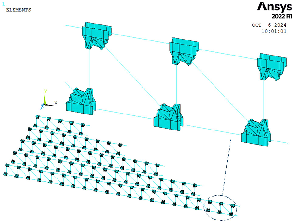
Beam and plate element model of steel truss.

Definition of rigid arm length coefficient

The rigid arm length in the ordinary beam element model, as shown in Figure 4, is determined based on the shape boundary of the nodal plate, and the cross-section used for the rigid arm closely resembles that of the bars outside the nodal plate domain. When the modulus of elasticity for the rigid arm is set to infinity, the resulting mid-span deflection calculated using this fully rigid arm is too small. On the other hand, when no rigid arm is applied, meaning the rigid arm is assigned a modulus of elasticity equal to that of the steel, the mid-span deflection calculated by this conventional model is excessively large.

Figure 4.

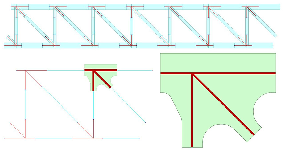
Setting of rigid arm length for ordinary beam element model.

To ensure that the stiffness of the rigid arm remains within a reasonable range, a modified rigid arm is defined here. This modified rigid arm achieves displacement equivalence by adjusting its length. The displacement equivalence can be matched either with the displacement results calculated by a high-precision plate element model or with the measured displacement of the truss.

Generally the modified rigid arms (L₁₂, L₂₂, L₃₂, L₄₂) are shorter than the lengths of the fully rigid arms (L₁₁, L₂₁, L₃₁, L₄₁) because the nodal plate contributes to the overall stiffness, acting like the web of the bar. The bar stiffness is still relatively small when the height of the web has not increased significantly. In Figure 5, the shaded portion represents the nodal plate region, which should be deducted from the rigid arm length because its stiffness is similar to that of a normal bar. When considering the stiffness individually for the four bars, the rigid arm length coefficient is defined as follows:

$${\eta }_i=L_{i2}/L_{i1}$$

(1)

Figure 5.

Setting of correcting rigid arm length.

In this context, i represents the serial number of the first to fourth rods, and the η _i values for each rod are not identical due to the differing shapes of the connecting ends of the nodal plates. By adjusting the rigid arm lengths according to the actual stiffness contribution of the nodal plate, this method provides a more accurate representation of structural behavior.

To simplify the calculation, a uniform η can be identified, which approximates each η _i as closely as possible while still achieving displacement equivalence. The subsequent calculations will be based on this simplified condition to determine the rigid arm length coefficient η.

Bayesian statistical theory

When there are fewer feature parameters, the probability table and decision tree generated by Bayesian theory are relatively simple, making them effective tools for predicting the rigid arm length coefficient η. By defining two-dimensional random variables (Y = i, X = j), the conditional probability is given by:

$$P(Y=i|X=j)=\frac{P(Y=i,X=j)}{P(X=j)}$$

(2)

The equation provided illustrates that the conditional probability is equal to the joint probability divided by the marginal probability. In turn, the joint probability can be calculated using the multiplication rule of probability:

$$\begin{array}{c}\multicolumn{1}{c}{P(Y=i,X=j)=P(Y=i|X=j)P(X=j)}\\ =P(X=j|Y=i)P(Y=i)\hfill \end{array}$$

(3)

Before performing Bayesian theory calculations, it is important to conduct feature screening of all defined parameters to identify those that are highly correlated with the predicted labels. Pearson’s correlation coefficient is a commonly used statistic for measuring the strength and direction of the linear relationship between two variables. The coefficient takes values ranging from −1 to 1, where:

• A value of 0 indicates no correlation between the two variables.

• A value close to 1 indicates a strong positive correlation, meaning as one variable increases, the other tends to increase as well.

• A value close to −1 indicates a strong negative correlation, meaning as one variable increases, the other tends to decrease.

The Pearson correlation coefficient ρ is calculated as follows:

$$\rho =\frac{\sum _{i=1}^n(X_i-\overline{X})(Y_i-\overline{Y})}{\sqrt{\sum _{i=1}^n{(X_i-\overline{X})}^2{(Y_i-\overline{Y})}^2}}$$

(4)

Where:

$X_i$ and $Y_i$ represent the individual data points for the two variables.

$\overline{X}$ and $\overline{Y}$ are the means of the variables $X$ and $Y$ , respectively.

ANN neural networks

The architecture of artificial neural networks (ANN) is generally straightforward, but in the early stages, uncertainty in the direction of iteration posed significant challenges for updating the weights. It wasn’t until the development of the backpropagation algorithm, coupled with the chain rule that simplified the derivation process for complex networks, that the solution of ANN networks became stable and reliable.

ANNs are particularly effective at establishing nonlinear relationships between predicted labels and multiple feature parameters. In this context, the rigid arm length coefficient η is nonlinearly related to the size parameters defined earlier, making ANNs well-suited for accurately modeling this relationship. By leveraging the backpropagation algorithm, ANNs can iteratively adjust the weights in the network, minimizing the error between the predicted and actual values, and ultimately providing a robust prediction model for η.

In this architecture as shown in Figure 6, the number of input neurons is defined as 11, corresponding to the feature parameters (ns, h1, …, tk). These feature parameters are normalized and organized into a column vector [X]. Subsequently the neurons in the hidden layers are responsible for integrating and downscaling the output of the signals, the first hidden layer collects the signals [Z(1)] after multiplying the column vectors [X] and their respective weights [W(1)], and the bias [b(1)] is used for the overall bit-potential adjustment of the signals. The hyperbolic tangent activation function processes the signal to obtain tanh([Z]), the output layer and the second hidden layer then repeat the process of the first hidden layer weights [W] and bias [b], and the final output tanh([Z]) is a predicted label value. After three layers of full link nesting, this architecture has the ability to process nonlinear data in depth.

$$\begin{array}{c}\multicolumn{1}{c}{\left[X\right]=\left[\begin{array}{c}\begin{array}{c}\begin{array}{c}{x}_1\hfill \\ \multicolumn{1}{c}{x_2}\\ \multicolumn{1}{c}{x_3}\\ \multicolumn{1}{c}{x_4}\end{array}\hfill \\ \multicolumn{1}{c}{x_5}\\ \multicolumn{1}{c}{x_6}\\ \multicolumn{1}{c}{x_7}\end{array}\hfill \\ \multicolumn{1}{c}{x_8}\\ \multicolumn{1}{c}{x_9}\\ \multicolumn{1}{c}{\begin{array}{c}{x}_{10}\hfill \\ \multicolumn{1}{c}{x_{11}}\end{array}}\end{array}\right]=\left[\begin{array}{c}\begin{array}{c}\begin{array}{c}\mathrm{ns}\hfill \\ \multicolumn{1}{c}{h1}\\ \multicolumn{1}{c}{\mathrm{ht}1}\\ \multicolumn{1}{c}{\mathrm{wt}1}\end{array}\hfill \\ \multicolumn{1}{c}{w}\\ \multicolumn{1}{c}{h2}\\ \multicolumn{1}{c}{\mathrm{ht}2}\end{array}\hfill \\ \multicolumn{1}{c}{\mathrm{wt}2}\\ \multicolumn{1}{c}{r}\\ \multicolumn{1}{c}{\begin{array}{c}\mathrm{dp}\hfill \\ \multicolumn{1}{c}{\mathrm{tk}}\end{array}}\end{array}\right]}\end{array}$$

(5)

$$[Z^{\left(1\right)}]=[W^{\left(1\right)}][X]+[b^{\left(1\right)}]$$

(6)

$$[Z^{\left(2\right)}]=[W^{\left(2\right)}]\tanh ([Z^{\left(1\right)}])+[b^{\left(2\right)}]$$

(7)

$$\eta ={Z_1}^{\left(3\right)}=[Z^{\left(3\right)}]=[W^{\left(3\right)}]\tanh ([Z^{\left(2\right)}])+[b^{\left(3\right)}]$$

(8)

Figure 6.

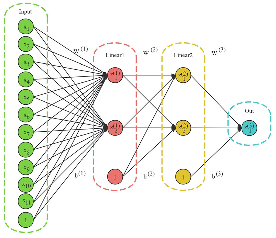
ANN neural network architecture.

Once the architecture of the neural network is determined, Mean Squared Error (MSE) is chosen as the error evaluation metric for the model. MSE is calculated as the average of the squared differences between the predicted values and the actual values:

$$\mathrm{MSE}=\frac{1}{n}\sum _{i=1}^n{({\hat{y}}_i-y_i)}^2$$

(9)

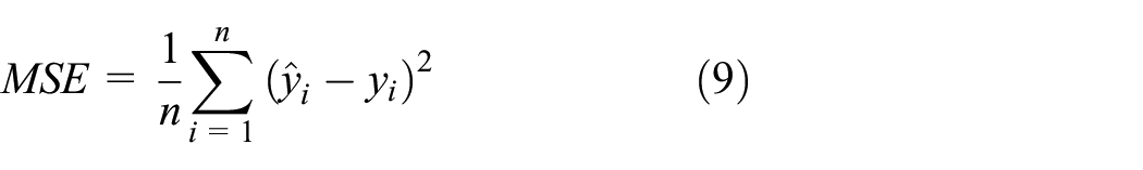
Where:

$n$ is the number of data points,

$y_i$ represents the actual value for the i-th data point,

${\hat{y}}_i$ represents the predicted value for the i-th data point.

To minimize the MSE, the Stochastic Gradient Descent (SGD) optimization algorithm is used to efficiently find the stationary points of the weights. The core of neural network backpropagation involves computing the gradient of the MSE loss function with respect to the weights w. This gradient is then multiplied by the step size s (also known as the learning rate) to update the weights w:

$$v_{(t)}=m{v}_{(t-1)}-s\frac{\partial \mathrm{MSE}}{\partial w}$$

(10)

However, during the backpropagation process, neural networks often tend to converge to local minima, which may not be the best solution for minimizing the loss function. To help the model escape from these local minima and move toward the global minimum, a momentum term m is introduced. The momentum adjusts the size of the historical gradient v_(t−1) to influence the current weight update.

$$w_{(t+1)}=w_{\left(t\right)}+v_{\left(t\right)}$$

(11)

Modeling results

Results of dataset construction

To achieve the computational accuracy of a plate element model with a beam element model, it is necessary to train the rigid arm parameters of the beam element model using a large dataset derived from the plate element model. Initially, the influence of each parameter on the rigid arm length was assessed using a smaller dataset model. Following this, the values of the five key parameters (ns, ht1, ht2, r, tk) were refined to improve the precision of the model.

Under the application of a simply supported boundary condition and a 10,000 kN vertical force applied to the mid-span vertical rod, the high-precision plate element model produced mid-span deflection results, as shown in Figure 7. This setup provides a comprehensive dataset of 2,278,125 samples, with each sample consisting of 11 features and 1 label as shown in Table 2.

Figure 7.

Overall computational flow for η prediction by machine learning methods based on digital twin models.

Table 2.

Twin parameter settings (mm).

ns	h1	ht1	wt1	w	h2	ht2	wt2	r	dp	tk	Mid-span deflection
20	2100	45	45	1706	1304	45	45	1304	2413	70	Max = −2102
16	/	40	/	/	/	40	/	2108	/	65	/
12	1600	35	35	1121	905	35	35	804	1214	60	/
8	/	30	/	/	/	30	/	553	/	55	/
4	1100	25	25	536	505	25	25	303	15	50	Min = −8
Total sample size: $2278125=5\times 3\times 5\times 3\times 3\times 3\times 5\times 3\times 5\times 3\times 5$

Figure 7 shows the overall computational flow for η prediction by machine learning methods based on digital twin models, its core idea is to match the displacement of the beam element model and high-precision plate element by adjusting the length of the rigid arm.

To minimize the deviation of the rigid arm model from the deflection of the high-precision plate element model, the dichotomy method is employed to determine the appropriate rigid arm length that meets the specified accuracy requirements. In this approach, a specific coefficient η is introduced to shorten the rigid arm length, with η taking values in the range of 0.1–1.

• When η = 0.1, the rigid arm length is reduced to one-tenth of its original value.

• When η = 1, the rigid arm length is kept at its original value.

The goal is to adjust η such that the deflection deviation between the rigid arm model and the plate element model is within 2%. The value of η that satisfies this condition is considered to be within the target domain. Figure 8 shows the trend in the number of samples that fall outside the target domain as the search accuracy increases. With each iteration, the computational accuracy of η is doubled, which significantly improves the precision of the results. However, this process is computationally intensive, taking 3–5 days to run all the more than 2 million models.

Figure 8.

Trend of the number of rigid arm samples outside the target domain with search accuracy.

After several iterations, the deflection deviations calculated by the rigid arm model were reduced to within 2%, as if confined within the boundaries of a funnel, as illustrated in Figure 9. Through this process, a set of features and labels for machine learning, as shown in Table 3, was created.

Figure 9.

Deflection deviation at mid-span using rigid arm length coefficient.

Table 3.

Datasets for machine learning (mm).

Order	$\mathrm{ns}$	$h1$	$\mathrm{ht}1$	$\mathrm{wt}1$	$w$	$h2$	$\mathrm{ht}2$	$\mathrm{wt}2$	$r$	$\mathrm{dp}$	$\mathrm{tk}$	Deflection		Error (%)	$\eta$
												①	②
1	4	1100	25	25	536	505	25	25	303	15	50	−51.1	−51.6	1.0	47/128
2	4	1100	25	25	536	505	25	35	303	15	50	−46.5	−46.4	0.2	49/128
3	4	1100	25	25	536	505	25	45	303	15	50	−43.2	−43.4	0.5	32/128
4	4	1100	25	25	536	505	30	25	303	15	50	−48.8	−48.8	0.0	45/128
5	4	1100	25	25	536	505	30	35	303	15	50	−44.9	−45.3	0.9	31/128
⋮		⋮	⋮	⋮	⋮	⋮	⋮	⋮	⋮	⋮	⋮	⋮	⋮	⋮	⋮
2,278,121	20	2100	45	45	1706	1304	40	35	1304	2413	70	−412.3	−419.1	1.7	73/128
2,278,122	20	2100	45	45	1706	1304	40	45	1304	2413	70	−410.2	−416.0	1.4	67/128
2,278,123	20	2100	45	45	1706	1304	45	25	1304	2413	70	−414.5	−411.6	0.7	70/128
2,278,124	20	2100	45	45	1706	1304	45	35	1304	2413	70	−411.9	−417.8	1.4	64/128
2,278,125	20	2100	45	45	1706	1304	45	45	1304	2413	70	−409.9	−413.5	0.9	63/128

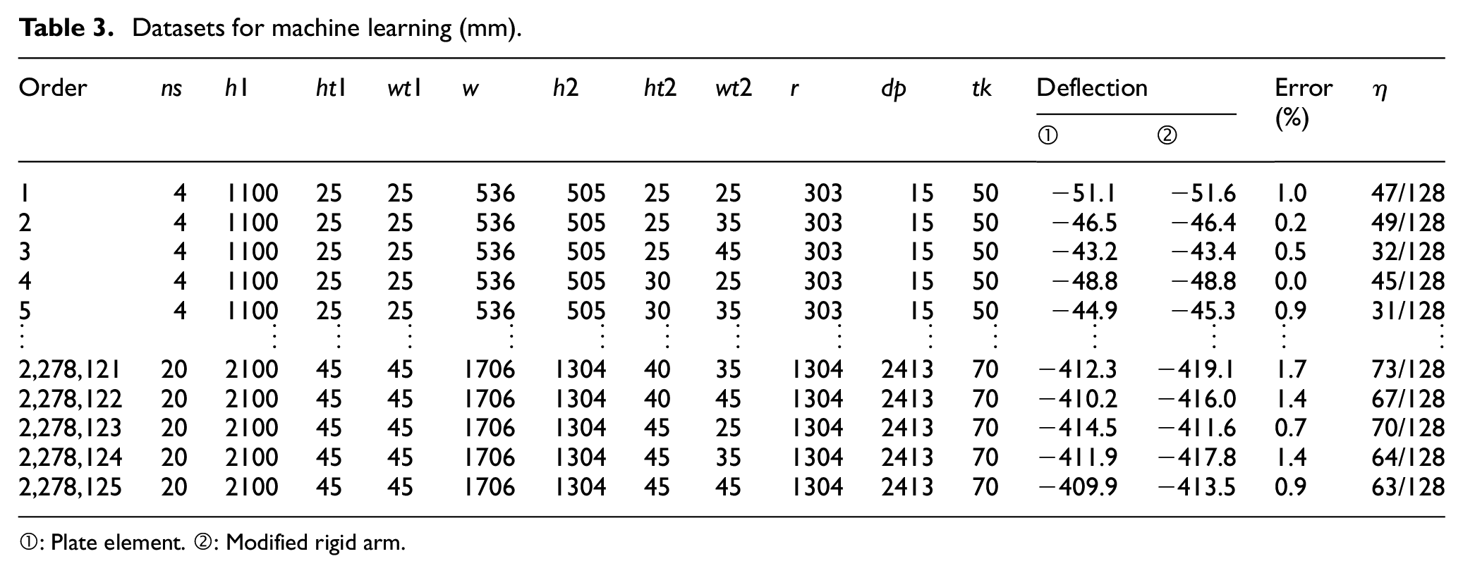
①: Plate element. ②: Modified rigid arm.

Bayesian-decision tree prediction results

Table 4 and Figure 10 shows the distribution of features and labels, and eta is basically a normal distribution. Its mean is 0.5018 and the standard deviation is 0.1718. The overall dataset has no missing values, does not require preprocessing, and normalization has a minimal impact on model training. The last column presents the Pearson correlation coefficients of each feature with the predicted labels, revealing that most features have minimal impact on the rigid arm length coefficient η, except for three features: (ns, ht1, tk). These three features show a significant correlation with η, indicating they play a crucial role in determining the rigid arm length. In contrast, other features, particularly the insertion depth dp, have a negligible effect on η. This suggests that the depth of the web rod’s insertion into the nodal plate does not significantly influence the rigid arm length. Whether the web insertion is shallow, or even if the web in the nodal plate region lacks top and bottom plates, the crossover node connected by the overall nodal plate can still be considered a rigid node.

Table 4.

Statistical indicators of features and labels (m).

Features and labels	Missing values	Unique values	Minimum	Maximum	Median	Mean	Standard deviation	η Correlation coefficient
ns	0	5	4	20	12	12	5.6569	0.474
ht1	0	5	0.025	0.045	0.035	0.035	0.0071	−0.462
tk	0	5	0.05	0.07	0.06	0.06	0.0071	0.442
w	0	9	0.5363	1.7063	1.0238	1.04	0.3441	−0.129
ht2	0	5	0.025	0.045	0.035	0.035	0.0071	−0.107
wt1	0	3	0.025	0.045	0.035	0.035	0.0082	−0.102
r	0	45	0.3029	1.3041	0.6747	0.6912	0.2343	0.093
wt2	0	3	0.025	0.045	0.035	0.035	0.0082	−0.064
dp	0	134	0.0151	2.4126	0.6279	0.6515	0.5766	−0.036
h1	0	3	1.1	2.1	1.6	1.6	0.4082	−0.036
h2	0	9	0.5049	1.3041	0.864	0.864	0.2460	−0.007
η	0	128	0	1	0.5	0.5018	0.1748	1

Figure 10.

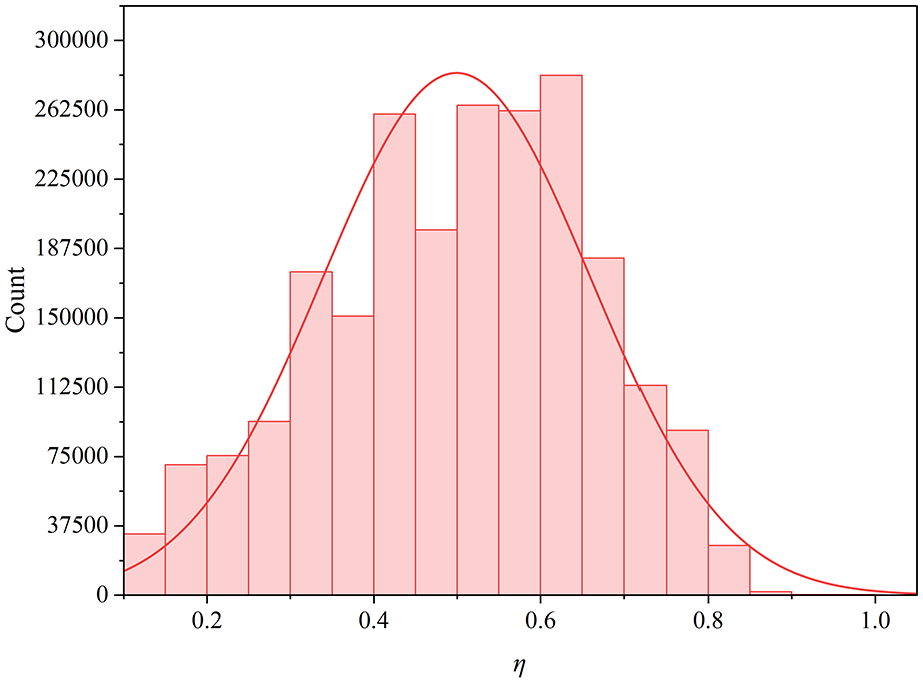
Distribution of η.

The probabilistic method can be employed to organize the samples by merging and categorizing them in advance, which reduces the overall number of samples. While this approach may lower the accuracy of the calculated rigid arm length coefficient η, the level of accuracy remains sufficient for most engineering applications. The joint probability of (ns, η) is easily obtained by the exhaustive method as shown in Table 5.

Table 5.

(ns, η) joint probabilities.

Confidence Interval		η × 16							Total
		0–3	3–5	5–7	7–9	9–11	11–13	13–16
$\mathrm{ns}=4$	n	41,721	24,666	62,966	14,168	15,079	410	5015	164,025
	p (%)	5.1	3.0	7.7	1.7	1.8	0.0	0.6	20.0
$\mathrm{ns}=8$	n	7920	10,750	52,089	29,190	54,984	6619	2473	164,025
	p (%)	1.0	1.3	6.4	3.6	6.7	0.8	0.3	20.0
$\mathrm{ns}=12$	n	2309	8244	39,357	25,788	66,554	13,588	8185	164,025
	p (%)	0.3	1.0	4.8	3.1	8.1	1.7	1.0	20.0
$\mathrm{ns}=16$	n	569	7153	34,619	23,906	68,643	16,398	12,737	164,025
	p (%)	0.1	0.9	4.2	2.9	8.4	2.0	1.6	20.0
$\mathrm{ns}=20$	n	120	5822	32,956	23,358	68,582	17,927	15,260	164,025
	p (%)	0.0	0.7	4.0	2.8	8.4	2.2	1.9	20.0
Total	n	52,639	56,635	221,987	116,410	273,842	54,942	43,670	820,125
	p (%)	6.4	6.9	27.1	14.2	33.4	6.7	5.3	100.0

The probability of correctly predicting the rigid arm length coefficient η to be within the range of 9/16–11/16 without considering any specific conditions is 33.4%. This percentage represents the marginal probability for column. Similarly, the probability of independently selecting any ns models is 20.0%, which also represents the marginal probability for that row in the probability table.

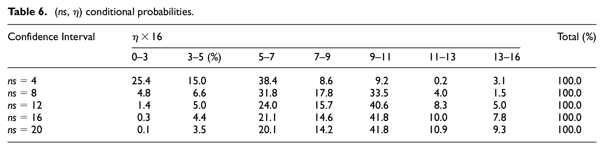
When considering the ns as a conditional factor, the prediction accuracy for η within the 9/16–11/16 range improves to 41.8% when ns equals 20 or 16. Table 6 shows how incorporating the conditional probability based on ns can significantly enhance the accuracy of predicting η. However, when ns = 4, the prediction for η shifts from the 9/16–11/16 range to the 5/16–7/16 range, with the accuracy for this prediction being 38.4%. This indicates that different ns (the number of sections in the truss) impact the likelihood of η falling within specific ranges, highlighting the importance of considering conditional probabilities in the prediction process.

Table 6.

(ns, η) conditional probabilities.

Confidence Interval	η × 16							Total (%)
	0–3	3–5 (%)	5–7	7–9	9–11	11–13	13–16
$\mathrm{ns}=4$	25.4	15.0	38.4	8.6	9.2	0.2	3.1	100.0
$\mathrm{ns}=8$	4.8	6.6	31.8	17.8	33.5	4.0	1.5	100.0
$\mathrm{ns}=12$	1.4	5.0	24.0	15.7	40.6	8.3	5.0	100.0
$\mathrm{ns}=16$	0.3	4.4	21.1	14.6	41.8	10.0	7.8	100.0
$\mathrm{ns}=20$	0.1	3.5	20.1	14.2	41.8	10.9	9.3	100.0

Introducing the decision condition ht1 (chord web thickness) into the model allows for a more refined prediction of the rigid arm length coefficient η. By analyzing the frequency response cloud plots under the two combined conditions of (ns, ht1), as shown in Figure 11, we can observe how these parameters interact to influence the prediction of η.

Figure 11.

Frequency response cloud plots for (ns, ht1) combination conditions.

In the cloud plots, the green dashed narrow channel represents a region where the frequency of certain η values is high. By selecting the η prediction value from this high-frequency region, the accuracy of the prediction improves to 46.2%. This approach leverages the concentration of data points in a specific range, leading to a more precise prediction. However, if the model allows for some reduction in accuracy, the η prediction region can be expanded. By enlarging the prediction region by a factor of 2, and using the wider channel indicated by the red dashed line, the prediction accuracy significantly increases to 65.6%.

The prediction accuracy of η can be significantly enhanced by introducing the decision condition tk (nodal plate thickness) in addition to ns and ht1. The strategy for determining the value of η under this three-layer decision condition is illustrated in Figure 12. By considering these three key parameters (ns, ht1, tk) in a decision tree model, the prediction accuracy increases substantially to 86.9%. However, adding more layers beyond these three does not yield substantial improvements in prediction accuracy. This is because the remaining features contain less relevant information and have a more limited impact on η.

Figure 12.

Decision tree for the (ns, ht1, tk) combination condition (η is magnified 16 times in the figure).

ANN neural network prediction results

The SGD optimization method is used to train the model based on the ANN architecture defined in this paper, with a batch size of 128, a learning rate of 0.035, and a momentum of 0.1. As shown in Figure 13, after 2000 epochs of training, the mean squared error (MSE) between the predicted and actual values in the test set converges to around 0.005. This low MSE indicates that the model has effectively learned the patterns and can make accurate predictions.

Figure 13.

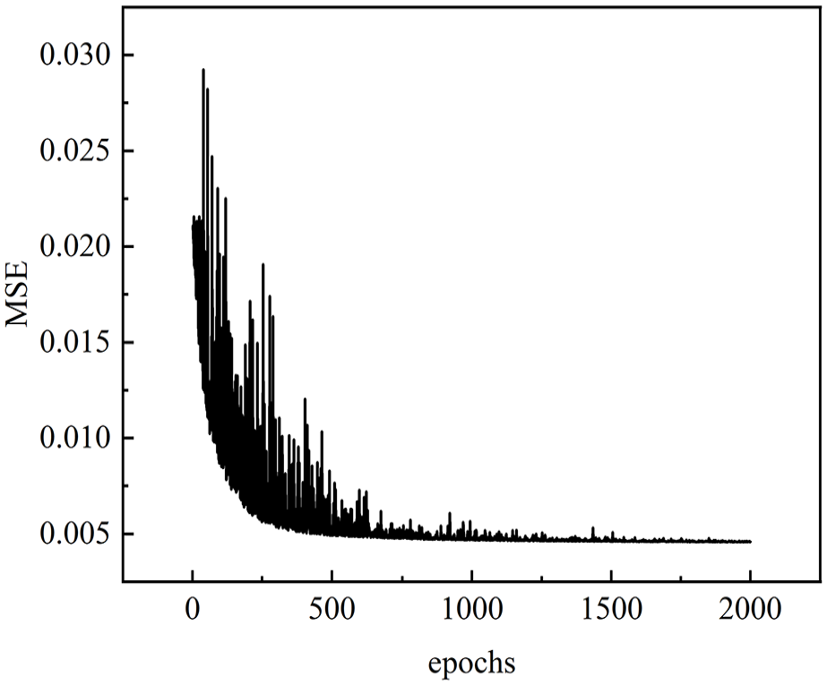
Test set MSE post-training trend.

At this point, the coefficient matrix of the neural network, which includes the weights and biases learned during training, is provided in equations (12)–(17). These coefficients are crucial for the network’s ability to process input data and generate predictions. The fact that this set of coefficients demonstrates strong generalization ability on the test set suggests that the neural network is not only fitting the training data well but is also capable of accurately handling unseen data, which is critical for its application in real engineering scenarios.

Coefficient matrix:

$$\left[W^{(1)}\right]=\left[\begin{array}{ccccccccccc}\begin{array}{c}0.1572\hfill \end{array}\hfill & 0.3413\hfill & -3.6750\hfill & 1.9355\hfill & -0.0717\hfill & -1.2267\hfill & -13.5310\hfill & -6.3243\hfill & 1.2403\hfill & -0.0190\hfill & 13.4510\hfill \\ \multicolumn{1}{c}{-0.0015}& -0.0561\hfill & -24.4400\hfill & -4.9513\hfill & -0.2433\hfill & 0.0215\hfill & -3.0256\hfill & -1.5104\hfill & 0.3177\hfill & -0.0420\hfill & 21.1930\hfill \end{array}\right]$$

(12)

$$[b^{\left(1\right)}]=\left[\begin{array}{c}-0.0761\hfill \\ \multicolumn{1}{c}{0.5365}\end{array}\right]$$

(13)

$$[W^{\left(2\right)}]=\left[\begin{array}{cc}\begin{array}{c}0.7780\hfill \\ \multicolumn{1}{c}{-7.2631}\end{array}\hfill & \begin{array}{c}0.4843\hfill \\ \multicolumn{1}{c}{-4.0639}\end{array}\hfill \end{array}\right]$$

(14)

$$[b^{\left(2\right)}]=\left[\begin{array}{c}-1.6996\hfill \\ \multicolumn{1}{c}{2.8932}\end{array}\right]$$

(15)

$$[W^{\left(3\right)}]=\left[\begin{array}{cc}2.2004\hfill & 0.5637\hfill \end{array}\right]$$

(16)

$$[b^{\left(3\right)}]=[2.4938]$$

(17)

Generally, ANN neural network algorithms offer more advantages over Bayesian decision trees when dealing with large datasets. Even with a simple architecture, this network achieves significant improvements in both computational precision and accuracy. As shown in Table 7, further increasing the complexity of neural network models can substantially enhance the accuracy in calculating the rigid arm length coefficient η.

Table 7.

Evaluation of computational results of complex neural networks.

Algorithm	Framework of layer	$|\hat{\eta }-\eta |\le 0.1$ accuracy (%)	$|\hat{\eta }-\eta |\le 0.01$ accuracy (%)
Regression	11 × 2 × 2 × 1	91.5	73.1
	11 × 1000 × 1000 × 1	100.0	91.2
Classification	11 × 11 × 11 × 128	100.0	92.3
	11 × 1000 × 1000 × 128	100.0	98.7

However, in practical scenarios like construction sites, the availability of deep learning expertise and computational resources is often limited. This limitation directly reduces the applicability of complex neural network models in such environments. In contrast, the simpler neural network architecture, which still delivers high accuracy and precision, becomes more practical and advantageous due to its lower resource requirements and ease of deployment.

Modeling evaluation

Automatic machine learning comparison

Knime is a fast automated modeling tool, and its model library can be used to quickly determine the best-performing machine learning models. The models currently used for regression are mainly shown in Figure 14. The model running process proceeds from left to right: the Excel dataset is first read and undergoes column transformations, followed by normalization and splitting into training and testing sets. After various regression models learn and train the data, the final output consists of predicted values and evaluation scores.

Figure 14.

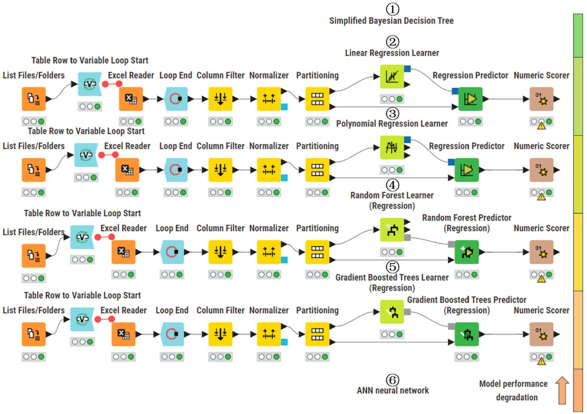
Automated machine learning process on the Knime platform.

According to the results in Table 8, the models are ranked in order of increasing performance as follows: Simple Bayesian Decision Tree, Multiple Linear Regression, Polynomial Nonlinear Regression, Random Forest, Gradient Boosting Tree, and ANN Neural Network.

Table 8.

Automated machine learning prediction performance evaluation table.

Evaluation indicators	Model ①	Model ②	Model ③	Model ④	Model ⑤	Model ⑥
MSE	0.274	0.065	0.055	0.052	0.038	0.005
R 2	0.342	0.727	0.781	0.819	0.850	0.993

MSE is generally better when smaller, indicating that the average deviation between the model’s predicted values and the actual values is smaller. The closer the R-squared (R²) value is to 1, the better, as it indicates that the predicted pattern of the model closely matches the shape of the actual data distribution. This helps avoid situations where large local deviations are averaged out, resulting in a small MSE despite significant discrepancies.

Among them, the performance of the ANN neural network leads by a significant margin, while the Bayesian Decision Tree yields relatively average prediction results due to insufficient depth and number of branches. The MSE and R-squared results of the other automated machine learning models fall between those of the first two.

The Bayesian Decision Tree calculation process introduced in this paper only involves counting the distribution of statistical features and labels, and then calculating the probabilities using Bayes’ theorem to draw the decision tree diagram. This method is suitable for engineers with low learning cost requirements, as simple techniques often have high practical value.

The ANN neural network typically requires the deployment of a big data computing platform, a requirement that far exceeds the talent and knowledge reserves of most engineering construction organizations. However, the rigid arm length rule organized in this paper has been condensed into the formula 5–8, which significantly lowers the threshold for machine learning. As this paper is an application-oriented engineering study, it focuses on promoting the use of the Bayesian Decision Tree and ANN Neural Network.

Mutual authentication

Before analyzing the real bridge model, the accuracy of the two methods – Bayesian decision tree and ANN – was first verified by comparing their predictions. A total of 179,850 data points were randomly selected from the twinned dataset of 2,278,125 data points, and for each, a prediction value η was calculated using both methods. The number of ANN-predicted values falling within the Bayesian decision tree prediction intervals was then counted, along with the percentage of overlap.

As shown in Figure 15, nearly all of the η values predicted by the ANN method fall within the Bayesian decision tree’s prediction intervals, with more than 90% of the intervals overlapping. Additionally, when calculating nodal plates with relatively high stiffness – where the rigid arm length coefficient η approaches 1 – the predictions from both methods overlap by as much as 100%. This indicates that the predicted trends for real data are highly consistent between the two methods. In other words, the greater the overall stiffness of the nodal plate, the more accurate the prediction of the rigid arm length coefficient η.

Figure 15.

Statistical quantitative plot of prediction results for η by both Bayesian-Decision Tree and ANN neural network methods (η is magnified 16 times in the figure).

Model validation of bridge examples

The Xiangshan Bridge, a steel truss cable-stayed bridge with a main span of 880 m in the Pearl River Estuary, has successfully implemented integral nodal plate connection technology. The stiffness of these nodal plates can be effectively accounted for using the methods discussed in this paper. Figure 16 illustrates both the plate element model and the rigid arm model of the Xiangshan Bridge.

Figure 16.

Plate elements and modified rigid arm model of Xiangshan Bridge.

For this bridge, the Bayesian decision tree method suggests using a uniform rigid arm length coefficient of [7/16–11/16] for all nodal plates. In contrast, the coefficients calculated by the ANN neural network method vary, reflecting the more nuanced analysis provided by this approach. Specifically, there are 10 types of nodal plates in the center span of the bridge. The ANN method yields a mean η value of 0.53, with an extreme deviation of 0.1. In the side spans, where there are 13 types of nodal plates, the mean η value is calculated to be 0.43, with an extreme deviation of 0.12. The calculated parameters for the side-span and mid-span in the example are shown in Tables 9 and 10.

Table 9.

Values of η for the mid-span parameter condition (mm).

Order	ns	h1	ht1	wt1	w	h2	ht2	wt2	r	dp	tk	η (decision tree)	η (neural network)
1	20	1800	30	46	1200	1000	36	28	900	1300	50	0.5625	0.50
⋮	⋮	⋮	⋮	⋮	⋮	⋮	⋮	⋮	⋮	⋮	⋮	⋮	⋮
10	20	1800	22	24	1200	1000	36	28	900	1300	40	0.5625	0.55

Table 10.

Values of η for the side-span parameter condition (mm).

Order	ns	h1	ht1	wt1	w	h2	ht2	wt2	r	dp	tk	η (decision tree)	η (neural network)
1	20	1800	24	28	1200	1000	28	20	600	1100	44	0.5625	0.53
⋮	⋮	⋮	⋮	⋮	⋮	⋮	⋮	⋮	⋮	⋮	⋮	⋮	⋮
13	20	1800	30	46	1200	1000	36	28	600	1300	50	0.5625	0.44

To streamline the modeling process for the rigid arm lengths, the mean η values are used for both the center and side spans of the bridge. This approach simplifies the model while still maintaining a high degree of accuracy in the simulation of the nodal plate stiffness. This decision balances the computational complexity with practical applicability, making it easier to implement and manage the model, especially in real-world engineering tasks.

Figure 17 shows the Shap values for the features of the ANN neural network obtained by sampling from the overall dataset, with a sampling ratio set to 1/100. This helps reduce the time for secondary forward propagation in the neural network. The color of the scatter points represents the relative magnitude of the feature values, while the clustering of the points indicates the distribution of the features. The horizontal axis represents the Shap values, which indicate the impact of the features on the model output η.

Figure 17.

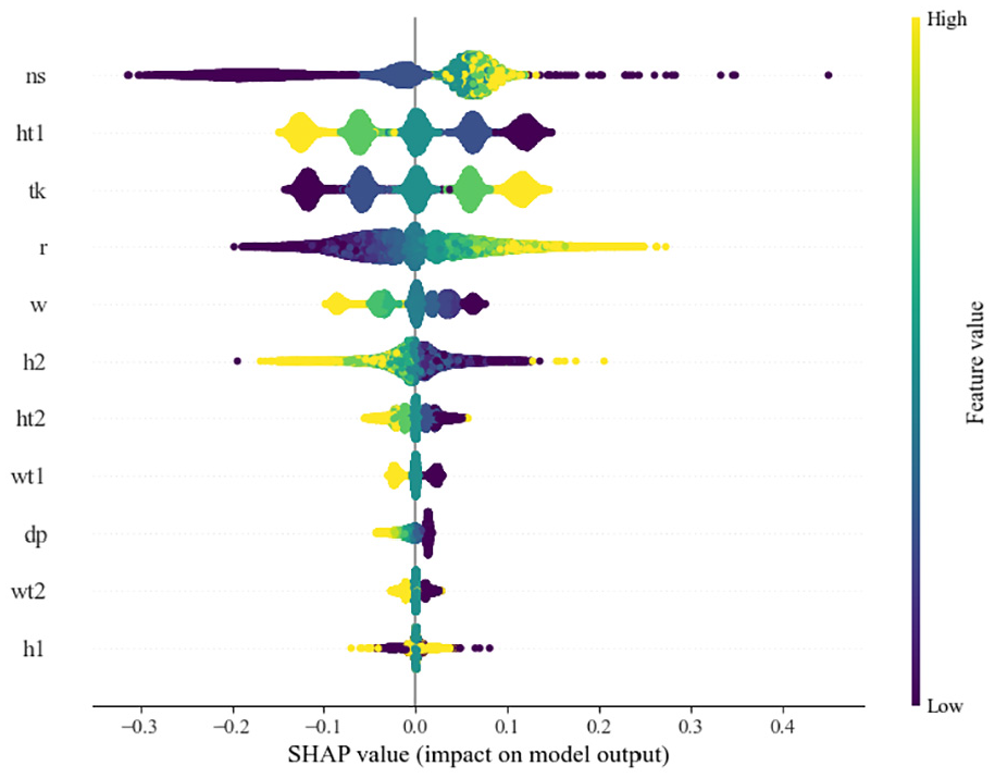
SHAP impact plot of node plate calculation parameters and η.

In the vertical arrangement, the importance of each feature decreases from top to bottom, with the three key features (ns, ht1, tk) being the most important, and the order of arrangement being consistent with the correlation coefficients shown in Table 4. The remaining features, which are determined to be unrelated to the label, also show significant impact in the Shap plot. This consideration of the joint effects between features is more reasonable than individually comparing the correlation between each feature and the label.

From the results shown in Figure 18, it is evident that the displacement of the bridge calculated using an ordinary beam element model is larger than that calculated with a fine plate element model. This discrepancy arises because the ordinary beam element model does not account for the stiffness of the nodal plates. In contrast, when the rigid arm length coefficient is calculated using an ANN neural network, the results are more accurate and closely match the fine plate element model, indicating that the ANN approach better captures the stiffness contributions of the nodal plates.

Figure 18.

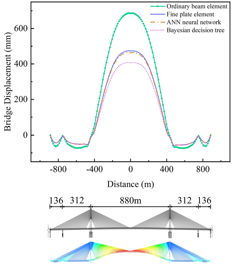
Calculation results of Xiangshan Bridge displacement.

On the other hand, the rigid arm length coefficient derived from the Bayesian decision tree method tends to be larger than that from the neural network. This leads to an overestimation of the overall bending stiffness of the steel truss, resulting in smaller calculated bridge displacements, particularly under the tension force of the diagonal cables at mid-span.

For large-span steel truss bridges, the ANN neural network is preferred for calculating the rigid arm length coefficient because of its superior accuracy in representing the nodal plate stiffness, which is crucial for ensuring the precision of the displacement calculations.

Conclusions

This paper, set against the backdrop of the Xiangshan Bridge steel truss girder project, presents the development of a digital twin parameter model for the overall nodal plate and provides recommendations for calculating the rigid arm length coefficient. Additionally, it introduces methods for predicting the rigid arm length coefficient using ANN neural networks and Bayesian decision trees. In summary, the results of these methods can effectively assist beam element modeling, significantly improving both work efficiency and calculation accuracy. The following key conclusions have been drawn:

• 1. Rigid arm length coefficient calculation method

The method proposed in this paper effectively addresses the issues of excessive deflection in traditional non-rigid arm models and insufficient deflection in fully rigid arm models. By appropriately matching the rigid arm length, this method improves the correction effect on displacement calculations in beam element models. The deflection results for the steel truss girder align well with those obtained from high-precision plate element models, which is beneficial for the construction control of steel truss girder alignment.

• 2. Neural network-based calculation method

The proposed method for calculating the rigid arm length using a neural network provides clear visibility into the hidden layers of the model, encapsulated in a formula. This approach is characterized by its simplicity, accuracy, and strong interpretability. Furthermore, the method is cost-effective in terms of training, making the neural network a highly convenient tool for bridge structure calculations.

• 3. Bayesian decision tree-based calculation method

Although the Bayesian decision tree-based method requires further improvement in precision and accuracy, it remains a useful, quick, and convenient method, particularly when there is a high correlation between feature values and labeled values. In the preliminary design phase, where most eigenvalues are not yet determined, a decision tree established with a small number of features can be effectively used to estimate nodal plate stiffness.

• 4. Shortcomings

The overall nodes of steel truss beams exist in various structural forms, such as T-shaped, N-shaped, K-shaped, and composite nodes. The arm length coefficient calculated by the formula summarized in this paper is only valid for N-shaped nodes. N-shaped nodes are the mainstream form used in steel truss cable-stayed bridges with main spans over 500 m. If other forms of nodes are used in medium and small-span steel truss beams, the calculation of the corrected arm length would require further targeted research.

• 5. Future directions

As more real-world datasets become available, there will be opportunities for deep training of neural networks, along with potential architectural adjustments. These advancements are expected to lead to even more accurate computations of the rigid arm length coefficient, further enhancing the reliability and applicability of the proposed methods.