Sage Journals: Discover world-class research

Abstract

Grinding is a critical method for enhancing the quality of worm tooth surfaces, and its process optimization has long been a significant research focus; however, existing methods are insufficient in addressing the nonlinearity and complexity inherent in the grinding of complex surfaces. In this study, a three-objective optimization function tailored for grinding complex spiral surfaces is developed and experimentally validated. We have successfully applied the innovative integration of the Multi-objective Grey Wolf Optimization Algorithm (MOGWO) and the optimization function to optimize the grinding process of the Roller Enveloping Worm Reducer (REWR). To account for actual working conditions, we developed constrained models for grinding ratio and machining rigidity and improved the boundary processing method for MOGWO optimization. The enhanced MOGWO demonstrates superior search capabilities during the optimization process, with its optimal solution outperforming traditional optimization algorithms. The optimized grinding process parameters reduce the grinding time by 17.41%, improve the grinding surface quality by 4.46%, and reduce the grinding cost by 1.12% compared with the conventional machining scheme. This provides practical guidance for optimizing the REWR and other complex surface grinding processes.

Keywords

Complex grinding process evolutionary algorithm multi-objective optimization Multi-objective Grey Wolf Optimization Algorithm production cost production rate

Introduction

Grinding is the final process to eliminate tooth surface deformation and achieve the desired geometric accuracy and surface quality.¹ Tooth surface roughness is a key grinding index, optimized by controlling machining factors. The Roller Enveloping Worm Reducer (REWR) is a novel transmission mechanism that transforms sliding friction into rolling friction.² It offers high precision and strong load capacity, making it useful in robotics, CNC machine tools, radar technology, aerospace, and more.^3,4 The complex contact surface of the REWR presents significant optimization challenges, often requiring extensive precision machining experiments for feedback. However, actual processing must also consider efficiency and economic benefits, making comprehensive optimization of processing factors essential for multi-objective improvement.⁵

Traditional grinding mechanism research forms the foundation of grinding optimization and plays a critical role. In their theoretical study of grinding processes, Dražumerič et al. proposed a novel unifying modeling framework to address the difficulty of modeling and quantifying abrasive tools during grinding, using the theory of aggressiveness.⁶ Setti et al. studied the trajectory of abrasive particles and their interaction with workpieces in micro-grinding, developed a theoretical undeformed chip thickness model.⁷ In experimental research on grinding processes, Guo et al. investigated the shape, size, posture, and distribution of CVD diamond grains and established an effective grinding wheel model to analyze and optimize the grinding process.⁸ Zhang et al. contributed significantly to the research on the grinding mechanism of diamond grinding wheels, establishing a new model for maximum undeformed chip thickness, which they verified through experiments.^9,10 They extensively studied the scratch grinding mechanism of individual grains and developed a new method for nanoscale cutting.¹¹ With the breakthrough of theory and experiment, many novel grinding methods have been developed.^12,13 These studies provide rich experience for the accurate control of grinding process and promote the development of the universality of grinding optimization.

Currently, controlling grinding processing factors relies heavily on engineers’ practical experience, requiring extensive trial and error, which impairs efficiency. To achieve high-quality, precise, efficient, and energy-efficient machining, engineers often use multi-objective nonlinear programming models to determine optimal machining parameters by studying the influence of process parameters. Traditional optimization models for grinding surface quality mainly use classical methods based on experimental data, such as quadratic programming with Multi-Criteria Decision Making (MCDM) techniques. For instance, Gao et al. developed a linear regression roughness prediction model based on diamond belt grinding data and optimized processing parameters by considering the material removal rate.¹⁴ Wang et al. analyzed gear grinding parameters using worm grinding wheels and established a quadratic regression model for tooth surface roughness. These traditional methods are inefficient and lack adaptability in solving mathematical models, highlighting the need for prediction models that do not rely on extensive experimental data for optimization.¹⁵ In studying multi-objective optimization models for the grinding process, Wen et al. proposed a three-objective model considering roughness, cost, and time, using quadratic programming with a weighted objective function to determine optimal grinding parameters.¹⁶ However, this algorithm’s limitations result in inexact Pareto solutions. Researchers have since applied more effective methods to improve computational model efficiency.^17–21 These methods typically transform multi-objective problems into single-objective ones, failing to provide true Pareto optimal solutions. The weighted sum approach only yields solutions within the convex hull of the solution space. In multi-objective problems, objectives often conflict, making it impossible to find a single solution that optimizes all objectives simultaneously.²²

To achieve precise Pareto solutions, researchers have applied various intelligent algorithms to optimization problems. Techniques such as Genetic Algorithm (GA),^23,24 Particle Swarm Optimization (PSO),^25,26 and Scatter Search algorithm (SS)²⁷ have been used for multi-objective problems in diverse machining operations. Recently, new intelligent optimization algorithms have also been applied to the grinding process. Alajmi et al. introduced a quantum computing-based method (QBOM) to solve the three-objective optimization problem of processing cost, time, and surface finish in grinding.²⁸ Khalilpourazari and Khalilpourazary used a metaheuristic multi-objective dragonfly algorithm, proposing an effective static penalty method to address complex constraints and find the Pareto optimal solution for the three-objective optimization in grinding.²⁹

The Multi-objective Grey Wolf Optimization Algorithm (MOGWO) used in this study is a swarm-based metaheuristic optimization algorithm. Metaheuristic methodologies are categorized into trajectory, evolutionary, and swarm-based methods.³⁰ Swarm-based methods like MOGWO can traverse the entire Pareto front and mitigate local optima issues. MOGWO effectively navigates multi-dimensional spaces, avoiding local optima by mimicking grey wolves’ social hierarchy and predatory behaviors. Comparisons with methods like Differential Evolution (DE) and Particle Swarm Optimization (PSO) show MOGWO’s superior performance.³¹ MOGWO also features rapid convergence, robust development, and a straightforward search mechanism.³² Innovations in grinding optimization models increasingly use intelligent optimization methods. Optimizing the roughness model requires extensive experiments to establish prediction models, often focusing on plane grinding. This study optimizes the grinding process for the complex spatial surface of the REWR. Traditional plane grinding models are inadequate for this, and the roughness varies across different positions, which renders the collection of large amounts of experimental data impossible.

In this study, several key components are considered for optimizing the worm grinding process. Section “Optimization model of tooth surface grinding” introduces a model for predicting worm tooth surface roughness, tailored for process optimization. A multi-objective optimization mathematical model is formulated, aiming to enhance machining efficiency, economic benefits, and tooth surface roughness. Section “Multi-objective optimization of worm grinding” utilizes the Grey Wolf Optimization Algorithm to solve this model, striving to achieve non-dominated Pareto solutions. The algorithm identifies optimal processing conditions while adhering to dynamic constraints, minimizing both cost and time while ensuring optimal surface roughness. Section “Results and discussion” employs the TOPSIS evaluation principle to consolidate and compare optimization outcomes, validating the effectiveness of the proposed Pareto optimal solutions through comprehensive analysis.

Optimization model of tooth surface grinding

Modeling of grinding roughness

As part of our comprehensive study on surface roughness in worm grinding, we have detailed the calculation principles applied in our model.³³ Surface roughness in grinding primarily results from furrows formed by the interaction between the abrasive cutting edge and the workpiece. Ono et al. analyzed grinding surface roughness geometrically, focusing on the movement trajectory of the abrasive cutting edge. They employed the concept of subsequent cutting edges and the analytical method from the theory of equal cutting height to analyze processed surfaces.³⁴ Zhu et al. investigated the impact of “plowing” on extrusion protrusions at groove ends.³⁵ This theory has been instrumental in predicting the roughness of grinding transmission structures, such as gears and face gears.^36–39 Equation (1) shows the proposed surface roughness prediction formula for REWR:

\begin{matrix} Ra = 0.256 (1 + \sqrt{\frac{1 - a_{b}}{2}}) {(\frac{15}{16})}^{0.4} Δ^{1.2} {(\cot θ_{0})}^{0.4} \\ {(\frac{v^{1' 2'}}{V} \sqrt{| \frac{1}{D} | \pm | \frac{1}{d} |})}^{0.4}, \end{matrix}

(1)

where V and $v^{1' 2'}$ are the velocities of the grinding head and the workpiece perpendicular to the grinding contact line, D and d represent the diameter of the grinding head and the workpiece at the contact point, “+” and “—“ are for cylindrical grinding and internal grinding, respectively, θ₀ is the conical half Angle of the top of the abrasive particles, whose statistical distribution can be obtained according to the type of abrasive particles,⁴⁰Δ is the average interval of the abrasive particles assumed to be uniformly distributed, a_b is the material removal rate.

During the grinding process of a worm, the interaction between the rotating grinding wheel and the rotating worm results in the formation of the tooth surface. The relative motion rate and contact curvature radius at the grinding contact points vary depending on the contact position, thereby producing a variety of grinding surfaces. Therefore, the grinding wheel contact point velocity can be expressed as:

V = 2 π NR,

(2)

where N is the rotational speed of grinding head, R is the radius of the roller. The velocity and angular velocity of the workpiece contact point can be expressed as follows:

\begin{matrix} v^{1' 2'} = ω_{1} \\ [R \sin (φ_{2}) + a \sin (θ) - (d_{2} - u) (i_{21} \cos (θ) + \sin (θ) \cos (φ_{2}))], \end{matrix}

(3)

ω^{1' 2'} = ω_{1} \sin (φ_{2}),

(4)

where θ is the worm rotation Angle, ω₁ is the worm angular velocity, ϕ₂ is the worm wheel Angle, d₂ represents the same radius of the worm gear tooth top circle as the grinding wheel, u is the height parameter of the grinding wheel, and i₂₁ is the transmission ratio.

Throughout the grinding process, a consistent grinding wheel is utilized to maintain alignment between the machined tooth surface and the theoretical tooth profile. As a result, the diameter of the grinding wheel varies at different grinding positions, and this variation can be expressed as:

D = - 2 R .

(5)

The REWR exhibits a more complex tooth surface, where the curvature of each contact point varies due to changes in the worm angle. This variation can be expressed as follows:

\begin{matrix} d = \frac{v^{1' 2'}}{ω^{1' 2'}} \\ = \frac{2 R \sin (φ_{2}) + a \sin (θ) - 2 (d_{2} - u) (i_{21} \cos (θ) + \sin (θ) \cos (φ_{2}))}{\sin (φ_{2})} . \end{matrix}

(6)

When measuring the tooth surface roughness of the REWR, the process involves calculating an arithmetic average within a specified range rather than point-to-point measurements. To align the surface roughness model of the REWR with the practical measurement method, the equation should be adjusted as presented in equation (7).

\bar{Ra} = \sum_{m = 1}^{n_{0}} (\sum_{m = 1}^{m_{0}} R a_{mn}) / i j,

(7)

where i and j are the length and width of unit sampling range, m₀ and n₀ are the number of sampling points on the i × j area.

Modeling of machining time

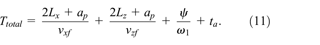
In worm grinding, the efficiency of the grinding tool system is evaluated by the processing time, which serves as a key metric. To enhance efficiency, the objective is to minimize the total processing time T_total mainly includes the machine tool’s no-load time t_nl, the material removal time t_g, and other auxiliary time t_a (including setup and standby periods of the grinder). Thus, the total time can be expressed by the equation²⁴:

T_{total} = t_{nl} + t_{g} + t_{a} .

(8)

No-load time

During the no-load phase in worm grinding, initiating spindle rotation is crucial to ensure consistent speeds for both the worm and the grinding wheel. Once stable speed is achieved, the grinding wheel undergoes a no-load feeding process until it makes contact with the worm. Following grinding, the operator performs a no-load cutting-back operation, and then stops the spindle. The brief start acceleration and stop deceleration times of the spindle are negligible in total time considerations. The no-load feed time t_nl can be divided into x axis feed return time t_xnl and z axis feed return time t_znl. Therefore, the no-load time can be expressed as:

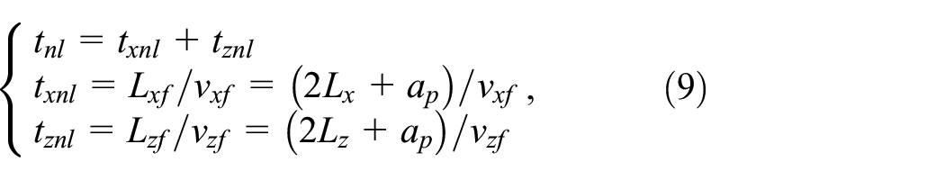
{\begin{matrix} t_{nl} = t_{xnl} + t_{znl} \\ t_{xnl} = L_{xf} / v_{xf} = (2 L_{x} + a_{p}) / v_{xf} \\ t_{znl} = L_{zf} / v_{zf} = (2 L_{z} + a_{p}) / v_{zf} \end{matrix},

(9)

where L_xf and L_zf are the feed and back-off distances of x-axis and z-axis; v_xf and v_zf are the feed and back speed of x axis and z axis; L_x and L_z are the x-axis and z-axis feed distances, a_p is the depth of grinding.

Material removal time

The material removal time in worm grinding refers to the duration during which the grinding wheel and the worm come into contact and subsequently separate. This duration is determined by the angular velocity of the worm and the total rotation angle:

t_{g} = \frac{ψ}{ω_{1}},

(10)

where ψ represents the total worm rotation Angle.

Other auxiliary time

As the grinding wheel makes prolonged contact with the worm tooth surface, its abrasive particles gradually wear down, necessitating regular dressing. Typically, dressing is manually conducted by operators based on experience, and its duration remains constant, unaffected by grinding parameters. Additionally, at the start of processing, activities such as machine tool startup, workpiece clamping, program and tool operation control are essential. Similarly, machine tool shutdown and workpiece disassembly occur upon completion, with the durations of these activities determined by pre-designed process parameters and remaining constant.

In summary, the grinding process time function is as follows:

T_{total} = \frac{2 L_{x} + a_{p}}{v_{xf}} + \frac{2 L_{z} + a_{p}}{v_{zf}} + \frac{ψ}{ω_{1}} + t_{a} .

(11)

Modeling of machining cost

This model focuses solely on the costs associated with the worm grinding process. Therefore, the total cost of the grinding process, denoted as C_total mainly comprises the following components: grinding fluid consumption cost C_gl, grinding wheel cost C_w, waste disposal cost C_h, grinding process energy cost C_e, equipment usage cost C_u, and labor cost C_l. Then the total cost can be expressed as follows:

C_{total} = C_{gl} + C_{w} + C_{h} + C_{e} + C_{u} + C_{l} .

(12)

Grinding fluid consumption cost

In worm grinding, despite recycling efforts, grinding fluid incurs losses through evaporation, adhesion to the workpiece, and contact with the grinding machine’s surfaces. Therefore, when accounting for the entire cycle from initial usage to replacement, the calculation of the grinding fluid cost is as follows:

C_{gl} = \frac{t_{nl} + t_{g}}{T_{cl}} V_{s} C_{pl},

(13)

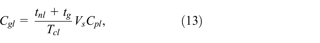
Where T_cl is the replacement cycle time of grinding fluid, C_pl is the unit volume cost of grinding fluid, V_s is the volume of grinding fluid under a single load.

Grinding wheel cost

The cost of the grinding wheel includes expenses for both wear and dressing incurred during the grinding operation. Macro wear of the grinding wheel involves deviations in shape, roundness, and edge passivation,⁴¹ which can significantly affect grinding efficiency and workpiece surface accuracy.⁴² Therefore, the formula for calculating the amount of wear is as follows⁴³:

Δ V_{g} = \frac{A L^{2} (1 + Doc / L) {F'}_{n} N}{{d_{e}}^{1.2 / VOL} VO L^{0.85}} \cdot t_{g},

(14)

VOL = 1.33 X + 2.2 S - 8,

(15)

where A is a constant and takes the value 0.0002, VOL is the wheel bonding percentage and the values of X are 0, 1, 2, …, for wheel hardness H, I, J, …. While S is the wheel structure number 4, 5, and 6. Doc is dressing depth, L is dressing advance, d_e is equivalent diameter of grinding wheel. $F'_{n}$ is that the grinding normal force changes with the grinding parameters, which is calculated by $F'_{n} = F'_{0} e^{- t / τ}$ .⁴³ $F'_{0}$ is the grinding force just before sparkout began, which is taken as 50 in this paper. The time constant $τ$ can be expressed by $τ = π du / K \cdot IWRP$ , K is the effective spring stiffness of the grinding system, IWRP can be obtained by equation (32). Therefore, the grinding normal force will change with the grinding parameters. The final grinding wheel cost can be expressed by the following formula:

C_{w} = \frac{Δ V_{g}}{G} k_{w} + \frac{C_{d}}{n_{D}},

(16)

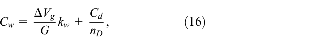
where G represents the grinding ratio of the grinding wheel, $G = G_{0} {(Q_{w} / 2 π NR)}^{- g}$ ,⁴⁴Q_w is the material removal rate per unit width, k_w is the price of grinding wheel per unit volume, C_d is the total cost of grinding wheel dressing, including power cost, loss cost, and labor cost, n_D is the number of grinding parts after dressing.

Waste disposal cost

During the grinding process, grinding waste is inevitably generated. Waste disposal is usually scheduled at regular intervals, where accumulated waste is centrally processed once it reaches a certain threshold. Therefore, the cost associated with waste disposal can be expressed as:

C_{h} = \frac{m_{r}}{m_{wr}} C_{wr} = \frac{ρ Δ V_{g}}{m_{wr}} C_{wr},

(17)

where m_r is the mass of waste slag produced by processing once, m_wr is the mass of waste slag processed once, C_wr is the cost of waste slag processed once, and ρ is the density of the workpiece.

Energy cost of grinding process

During the grinding preparation stage, the grinder consumes electrical energy, the amount of which varies based on the grinding conditions. Therefore, this component accounts for the electrical energy cost incurred specifically during the grinding process. The energy cost of the process is calculated as the product of the total energy consumption and the unit price of electricity. Hence, the cost can be expressed as follows:

C_{e} = \frac{E_{g}}{3.6 \times 10^{5}} C_{s},

(18)

where E_g is the energy consumption of machine grinding material removal, $E_{g} = \int_{0}^{t_{g}} p_{g} dt$ , where p_g is the material removal power, which is calculated by referring to the energy consumption formula established by Deng et al.,⁴⁵ and C_s is the unit price of electricity.

Equipment usage cost

The cost of equipment usage primarily reflects the value of significant fixed assets such as grinders and fixtures. Therefore, the cost associated with using these components is of primary concern. However, capital also carries a time value, and traditional depreciation methods may overlook this temporal aspect of asset valuation, potentially leading to significant inaccuracies and failing to objectively reflect the true value contribution of fixed assets.⁴⁶ In accordance with the time value theory of capital, the cost of using the grinding machine and grinding wheel can be expressed as follows²⁴:

\begin{matrix} {\begin{matrix} r_{i} = 2 (N_{s} - i) / N_{s} (N_{s} + 1), \\ Δ_{i} = (M_{k} - M_{L}) / r_{i}, \\ V_{n} = \sum_{i = 1}^{N - 1} Δ_{i} / {(1 + j)}^{i}, \\ S_{0} = (M_{k} - M_{L} - V_{n}) (S / V_{n}, j, N_{s} - 1), \\ Δ_{ri} = Δ_{i} + S_{0}, \\ C_{u} = \frac{T_{total}}{T_{cai}} Δ_{ri}, \end{matrix} \\ i = 1, 2, 3, \dots, N_{s} - 1, \end{matrix}

(19)

where r_i represents the depreciation rate in the ith year, N_s denotes the life cycle life of the grinder, Δ _i signifies the depreciation amount in the ith year without considering the time value of funds, M_k stands for the total value of grinders and grinding wheels, M_L indicates the salvage value after reaching the life cycle, V_n represents the net present value of grinding wheels and grinding wheels considering the time value of funds, j denotes the effective annual interest rate, S₀ represents the annuity, (S/V_n, j, N_s−1) is the present value coefficient of the annuity, and Δ _ri denotes the actual depreciation allocation. T_cai represents the total useful life in the ith year.

Labor cost

During the grinding operation, workers are required to perform the tasks and receive corresponding remuneration. Therefore, labor costs can be calculated based on hourly wages:

C_{l} = k_{h} T_{total},

(20)

where k_h is the operator’s hourly wage.

In summary, the multi-objective optimization function incorporating surface roughness, processing time, and processing cost as optimization objectives can be expressed as follows:

min F (ω_{1}, N, a_{p}) = (min Ra, min T_{total}, min C_{total}) .

(21)

Experimental setup

In the process of grinding worm tooth surfaces, setting parameters for processing time and cost models is complex, influenced by various uncertain factors including tool setup time, labor costs, and power expenses. This section focuses on validating the effectiveness of the roughness model. Further analysis of the morphological characteristics of the tooth surface was conducted through grinding experiments. Details of the experimental setup and measurements of the tooth surface are described in this section.

The worm grinding process and tooth surface measurement setup are depicted in Figure 1. To minimize the impact of machine feed errors on tooth surface roughness,⁴⁴ the worm blank was ground using a SCHNEEBERGER NORMA NGC grinder in Figure 1(a) and (b). The grinding process is illustrated in Figure 1(c), while Figure 1(d) and (e) exhibit the machined 20CrNiMo worm with a tooth height of 9 mm and a tooth surface hardness of 55–60HRC. To mitigate the effects of grinding wheel wear on surface topography after grinding, an alumina grinding wheel was employed, maintained through the self-sharpening process inherent to the grinding wheel and the dressing system of the machine tool. Detailed parameters of the worm and abrasive are provided in Tables 1 and 2.

Figure 1.

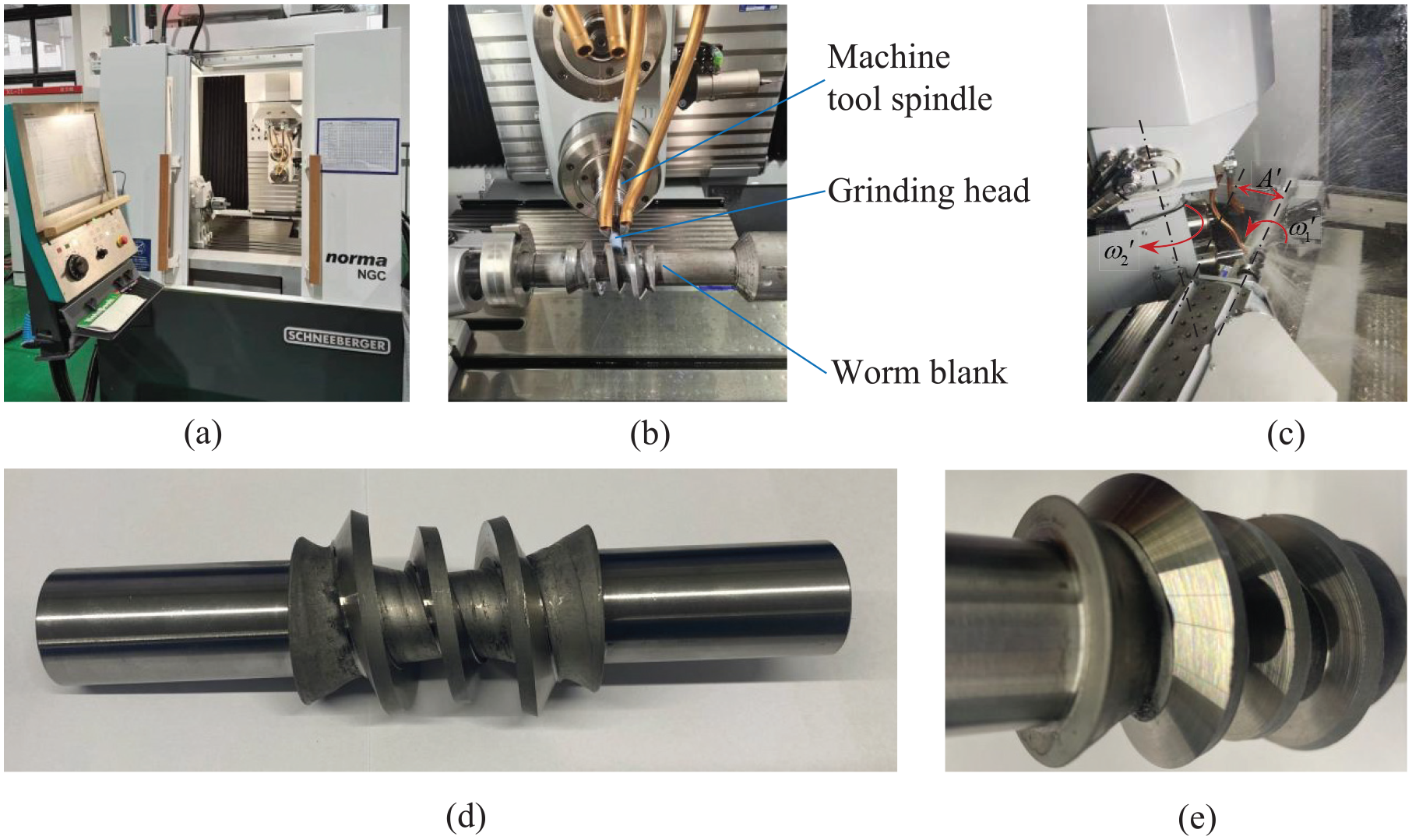
Experimental setup for grinding tests: (a) and (b) are the grinding machine machines; (c) shows the grinding process, (d) and (e) show the worm and tooth surface after grinding.³³

Table 1.

Experimental parameters of worm.

Worm parameter	Value
Center distance A (mm)	63
Roller radius R (mm)	5
Transmission ratio i₂₁	20
Full tooth height h₀ (mm)	9
Material	20CrNiMo
Tooth surface hardness	55–60 HRC

Table 2.

Experimental parameters of grinding tools.

Experimental parameter	Value
Radius R (mm)	5
Abrasive particle size M	100
Organization number S	6
Binding agent	Vitrified bonded
Abrasive material	Aluminum oxide
Rotation speed N (rpm)	16,000
Feed speed ω₁ (rad s⁻¹)	0.1
Feed speed ω₂ (rad s⁻¹)	0.005

To facilitate the measurement of the tooth surface, wire electrode cutting technology was employed to pre-cut the worm. As depicted in Figure 2(a) and (b), the worm was segmented into five sections along the axial direction and subsequently cleaned using ultrasonic waves. A contact line was taken on the tooth surface of each worm segment, distinguishing between the dedendum and addendum. In Figure 2(c), the surface morphology at the tooth root and tooth top positions of these contact lines was measured using a white light interferometer (Atometics-ER230). Detailed parameters measured are outlined in Table 3.

Figure 2.

Roughness measurement experiment: (a) the cutting dimension of the worm, (b) the worm after wire cutting, and (c) white-light interferometer.³³

Table 3.

Measurement parameters.

Measurement parameter	Value
Measurement equipment	White light interferometer (Atometrics-ER230)
Scanning height h (µm)	5000
Measurement accuracy s (nm)	0.1
Measured area S (µm)	450 × 450

In Figure 3(a) and (b), identical experimental parameters were employed for simulation to generate surface quality distribution diagrams of the left and right tooth surfaces. Observing the abrasive tool’s rotation around the center of revolution at varying angles during grinding, significant changes in the quality of the REWR surface are evident. Figure 3(c) and (d) illustrate expansion and mapping diagrams of surface roughness, indicating an irregular ribbon-like distribution pattern. Notably, the root of both left and right tooth surfaces exhibits lower roughness compared to the tooth tops, maintaining a consistent trend throughout. Table 4 provides surface roughness values (Sa) from experimental and simulated data at different positions under identical machining parameters. We observe a maximum error of 15.01% between simulated and experimental results, validating the accuracy of our surface roughness prediction model for worm tooth surface grinding.

Figure 3.

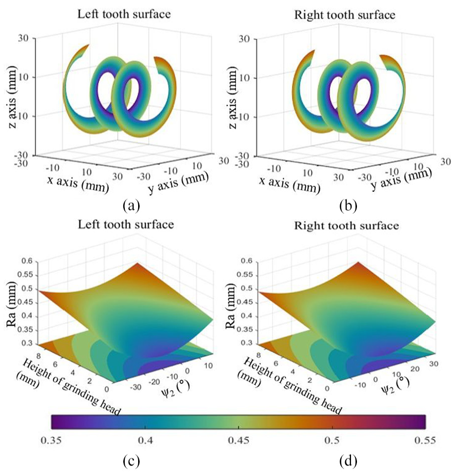
Simulation results of roughness distribution of tooth surface of worm: (a) and (b) represent the roughness distribution of the left and right tooth surfaces, (c) and (d) show the plane projection results along the height and feed angle of the grinding head.

Table 4.

Comparison of measured and calculated results.

Measuring position	Rotation speed n (rpm)	Wheel radius R (mm)	Measured Sa (μm)		Calculated Sa (μm)		Error (%)
Measuring position	Rotation speed n (rpm)	Wheel radius R (mm)	Dedendum	Addendum	Dedendum	Addendum	Dedendum	Addendum
1	16,000	5	0.473	0.457	0.4455	0.4823	5.81	5.54
2	16,000	5	0.356	0.381	0.393	0.4382	10.39	15.01
3	16,000	5	0.370	0.399	0.3747	0.4225	1.27	5.89
4	16,000	5	0.335	0.380	0.3774	0.4237	12.66	11.50
5	16,000	5	0.463	0.515	0.4358	0.4687	5.87	9.00

In Figure 4, the surface roughness of both the tooth root and the tooth top is depicted as a function of the grinding head’s machining angle. The striking similarity in the trends between experimental and simulation results suggests that our surface prediction model effectively captures the relationship between machining parameters and tooth surface topography.

Figure 4.

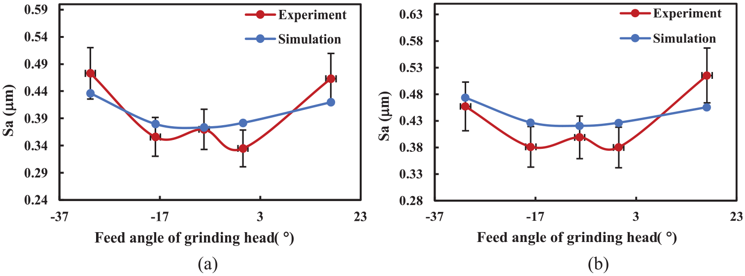
Comparison of Sa between experimental and simulation result: (a) dedendum of the worm tooth and (b) addendum of the worm tooth.

The observed disparity between measured and simulated results may be attributed to several unaccounted factors in our model. These include machine tool vibration, grinding wheel wear, and grinding wheel rigidity. Machine tool vibration can cause abrasive particles to deviate from their intended trajectory during cutting, leading to discrepancies between predicted and experimental outcomes. Furthermore, grinding wheel wear alters abrasive particle shape during grinding, introducing errors in surface topography predictions. Additionally, fluctuations in roughness observed at the third measurement position may stem from unique local material characteristics or the presence of impurities, among other factors. These elements contribute to inaccuracies in our measurement data.

Multi-objective optimization of worm grinding

This section initiates by defining constraint criteria tailored to the practical machining environment. A constraint model is developed that integrates the dynamics and contact relationships inherent in worm grinding, emphasizing parameters such as grinding ratio and machining stiffness to accurately reflect real-world machining influences. Next, we present a concise introduction to the classical Grey Wolf Optimization Algorithm (GWO) and its application in multi-objective optimization scenarios. This algorithm is chosen for its effectiveness in optimizing complex systems with multiple objectives. Lastly, we outline the specific optimization methodology adopted in this study, detailing our approach to integrating the constraint model with the GWO algorithm to achieve optimal machining outcomes.

Constraint setting

Processing condition constraints

As machining requirements and equipment specifications vary widely, determining the optimal range of machining variables relies heavily on production experience and the characteristics of the grinding equipment. This ensures that the results of model optimization are applicable to real-world machining scenarios. Surface roughness directly influences the operational stability and meshing accuracy of the worm. Key parameters such as grinding wheel speed, worm angular velocity, and grinding depth significantly impact the roughness of the worm tooth surface. During the actual grinding process, it is essential to maintain the spindle speed within the permissible range and ensure that operating power stays within rated limits. Operators should also adjust grinding allowances promptly to improve processing efficiency and reduce costs. Based on the above considerations, the constraints for the machining process can be summarized as follows:

g_{1} : \frac{π d_{0} n_{min}}{60000} \leq v_{s} \leq \frac{π d_{0} n_{max}}{60000}

(22)

g_{2} : ω_{min} \leq ω_{1} \leq ω_{max}

(23)

g_{3} : N_{min} \leq N \leq N_{max}

(24)

g_{4} : a_{p - min} \leq a_{p} \leq a_{p - max}

(25)

g_{5} : p \leq p_{e}

(26)

g_{6} : M \leq M_{max}

(27)

g_{7} : Ra \leq R a_{max}

(28)

g_{8} : C_{total} \leq C_{max}

(29)

where d₀ is the spindle diameter, $n_{min}$ and $n_{max}$ are the minimum and maximum values of the speed constraint, $ω_{1}$ is the worm angular velocity, $N_{min}$ and $N_{max}$ are the minimum and maximum values of the grinding wheel speed constraint, $a_{p - min}$ and $a_{p - max}$ are the minimum and maximum values of the cutting depth constraint, $P_{e}$ is the rated power of the machine tool, $M_{max}$ is the maximum value of the spindle torque constraint. $R a_{max}$ is the maximum value of surface roughness constraint, and $C_{max}$ is the maximum cost constraint.

Grinding ratio constraint

King and Hahn established a grinding ratio constraint based on surface grinding characteristics, defined as the ratio between the workpiece removal parameter WRP and the wheel wear parameter WWP.⁴³ This constraint is expressed as:

WRP = 94.4 (\frac{(1 + 2 Doc / 3 L) L^{11 / 19} {(v / V)}^{3 / 19} V}{d_{e}^{43 / 304} VO L^{0.47} d_{g}^{5 / 38} R_{c}^{27 / 19}}),

(30)

\begin{matrix} WWP = (\frac{k_{a} a_{p} d_{g}^{5 / 38} R_{C}^{27 / 19}}{d_{e}^{1.2 / VOL - 43 / 304} VO L^{0.38}}) \\ \times (\frac{(1 + Doc / L) L^{27 / 19} {(V / v)}^{3 / 19} v}{1 + 2 Doc / 3 L}), \end{matrix}

(31)

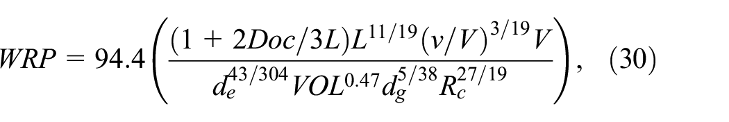
where d_g is abrasive size of grinding wheel, R_c is Rockwell hardness of workpiece, k_a is constant depending on coolant and grinding type of grinding wheel.

As the mathematical model is grounded in plane grinding, both velocity and contact curvature remain constant. However, the worm tooth surface of the REWR discussed in this paper presents a complex spatial surface, where contact rate and curvature vary across different positions. Therefore, combined with equations (2), (3), (5), and (6) above, the formula of improvement workpiece removal parameter IWRP and improvement wheel wear parameter IWWP suitable for complex space surface can be obtained:

\begin{matrix} IWRP = 94.4 (\frac{(1 + 2 Doc / 3 L) L^{11 / 19} {(v^{1' 2'} / 2 π NR)}^{3 / 19} 2 π NR}{VO L^{0.47} d_{g}^{5 / 38} R_{c}^{27 / 19}}) \\ {(| \frac{1}{2 R} | \pm | \frac{ω_{1} \sin (φ_{2})}{2 v^{1' 2'}} |)}^{43 / 304}, \end{matrix}

(32)

\begin{matrix} IWWP = (\frac{k_{a} a_{p} d_{g}^{5 / 38} R_{C}^{27 / 19} (1 + Doc / L) L^{27 / 19} {(2 π NR / v^{1' 2'})}^{3 / 19} v^{1' 2'}}{VO L^{0.38} (1 + 2 Doc / 3 L)}) \\ \times {(| \frac{1}{2 R} | \pm | \frac{ω_{1} \sin (φ_{2})}{2 v^{1' 2'}} |)}^{1.2 / VOL - 43 / 304} . \end{matrix}

(33)

Therefore, the constraint of grinding ratio G′ can be obtained as follows:

G' = IWRP / IWWP \geq G,

(34)

where G is the constant value of grinding ratio.

Machining stiffness constraints

During grinding, vibrations can induce corrugated roughness on the workpiece surface, compromising surface quality and meshing performance. To mitigate grinding chatter, reducing the workpiece removal rate is often necessary. Additionally, irregularities on the grinding wheel surface require frequent dressing. Therefore, ensuring stable conditions to prevent chatter is critical in selecting operating parameters. The relationship between grinding stiffness K_c, wheel wear stiffness K_s, and operating parameters during the whole grinding process is expressed as follows⁴³:

K_{c} = \frac{1000 d_{e}^{43 / 304} VO L^{0.47} d_{g}^{5 / 38} R_{c}^{27 / 19} f_{d} {(v / V)}^{16 / 19}}{94.4 (1 + 2 Doc / 3 L) L^{11 / 19}},

(35)

\begin{matrix} K_{s} = (\frac{1000 d_{e}^{1.2 / VOL - 43 / 304} VO L^{0.38} f_{d}}{k_{a} a_{p} d_{g}^{5 / 38} R_{C}^{27 / 19}}) \\ \times \frac{(1 + 2 Doc / 3 L) {(V / v)}^{16 / 19}}{(1 + Doc / L) L^{27 / 19}}, \end{matrix}

(36)

where f_d represents the z rate. Same as the grinding ratio constraint, the contact rate and curvature of the stiffness parameters also change in the grinding of the REWR tooth surface. The stiffness parameters are modified by combining formulas (2), (3), (5), and (6) above to apply to the complex space surface in this paper.

\begin{matrix} I K_{c} = \\ \frac{1000 VO L^{0.47} d_{g}^{5 / 38} R_{c}^{27 / 19} f_{d} {(v^{1' 2'} / 2 π NR)}^{16 / 19}}{94.4 (1 + 2 Doc / 3 L) L^{11 / 19} {(| 1 / 2 R | \pm | ω_{1} \sin (φ_{2}) / 2 v^{1' 2'} |)}^{43 / 304}}, \end{matrix}

(37)

\begin{matrix} I K_{s} = \\ \frac{1000 VO L^{0.38} f_{d} (1 + 2 Doc / 3 L) {(2 π NR / v^{1' 2'})}^{16 / 19}}{k_{a} a_{p} d_{g}^{5 / 38} R_{C}^{27 / 19} (1 + Doc / L) L^{27 / 19} {(| 1 / 2 R | \pm | ω_{1} \sin (φ_{2}) / 2 v^{1' 2'} |)}^{1.2 / VOL - 43 / 304}}, \end{matrix}

(38)

Based on the improved grinding stiffness and wheel wear stiffness proposed in this section, the corresponding machine static stiffness constraints are proposed as follows:

MSC = \frac{1}{2 I K_{c}} (1 + \frac{v}{VG}) + \frac{1}{I K_{s}} \geq \frac{| R_{em} |}{k_{m}} .

(39)

Multi-objective Grey Wolf optimization algorithm

Mirjalili et al.⁴⁷ introduced the classical Grey Wolf Optimization Algorithm as a novel population metaheuristic. Building upon this foundation, Mirjalili et al.⁴⁸ subsequently proposed the multi-objective Grey Wolf Optimization Algorithm. The algorithm mimics the strict leadership hierarchy of grey wolves in nature and their group hunting mechanism.

As illustrated in Figure 5, grey wolves are hierarchically divided into levels: α (alpha), β (beta), δ (delta), and ω (omega). Alpha holds dominance at the apex of the hierarchy, while Beta aids Alpha in exerting dominance and making supplementary decisions. Delta Wolf follows Beta and leads the omega-level wolves. Hunting behavior is mathematically modeled by defining new positions for all wolves in the pack based on the three leading wolves. Each wolf represents a solution to the optimization problem, while the group interaction symbolizes the optimization process. The search process of the Grey Wolf Optimizer (GWO) can be divided into the following two stages.

Figure 5.

The social hierarchy of a grey wolf pack.

Encircling prey

During hunting, grey wolves first surround prey. The bounding behavior can be mathematically defined below.

D = | C \cdot X_{P} (t) - X (t) |,

(40)

X (t + 1) = X_{P} (t) - A \cdot D,

(41)

where t is the index of the current iteration. X (t) and X (t+1) are the position vectors of ω Wolf in the current and next iteration, respectively. X _p (t) of t is the position vector of the prey. D can be viewed as the absolute distance vector between prey and candidate ω wolves. A and C are coefficient vectors with the following formula:

A = 2 a \cdot r_{1} - a,

(42)

C = 2 r_{2},

(43)

where a is a vector of length equal to X (t), whose components are linearly reduced from 2 to 0 during iterations to balance exploration and exploitation. r ₁ and r ₂ are random vectors with each element uniformly distributed at [0, 1]. It is worth noting that C is not linearly decreasing during the search process, which helps to improve explorability and avoid local optima.

Search for prey (exploration)

In the abstract search space, the optimal position of the prey, denoted as the limit position in equation (40), remains unknown. To mimic the hunting behavior of grey wolves, α, β, and δ are presumed to possess a better understanding of the potential location of the prey. Consequently, the Wolf updates its position based on α, β, and δ to initiate an attack on the prey. Mathematically, this hunting behavior is expressed as:

\begin{matrix} D_{α} = | C_{1} \cdot X_{α} - X (t) |, \\ D_{β} = | C_{2} \cdot X_{β} - X (t) |, \\ D_{δ} = | C_{3} \cdot X_{δ} - X (t) |, \end{matrix}

(44)

\begin{matrix} X_{1} = X_{α} - A_{1} \cdot D_{α}, \\ X_{2} = X_{β} - A_{2} \cdot D_{β}, \\ X_{3} = X_{δ} - A_{3} \cdot D_{δ}, \end{matrix}

(45)

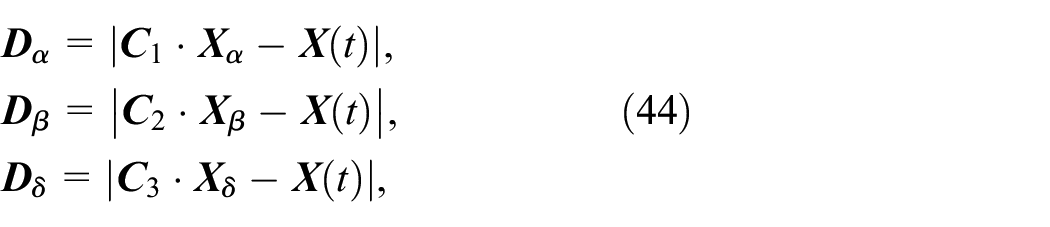
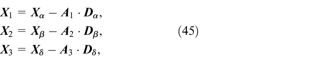
and

X (t + 1) = \frac{X_{1} + X_{2} + X_{3}}{3},

(46)

where A ₁ to A ₃ and C ₁ to C ₃ are random vectors generated by equations (42) and (43).

The Multi-objective Grey Wolf Optimization Algorithm (MOGWO) enhances the classical Grey Wolf Optimization Algorithm (GWO) with two novel components, reminiscent of those in MOPSO.⁴⁹ The first component is an archive that stores non-dominated Pareto optimal solutions obtained thus far. The second component involves a leader selection strategy that selects alpha, beta, and delta solutions from the archive to guide the hunting process. MOGWO’s computational complexity is comparable to NSGA-II,⁵⁰ MOPSO,⁴⁹ and PAES,⁵¹ and it surpasses algorithms like NSGA⁵² and SPEA.⁵³ Detailed calculations are illustrated in Figure 6.

Figure 6.

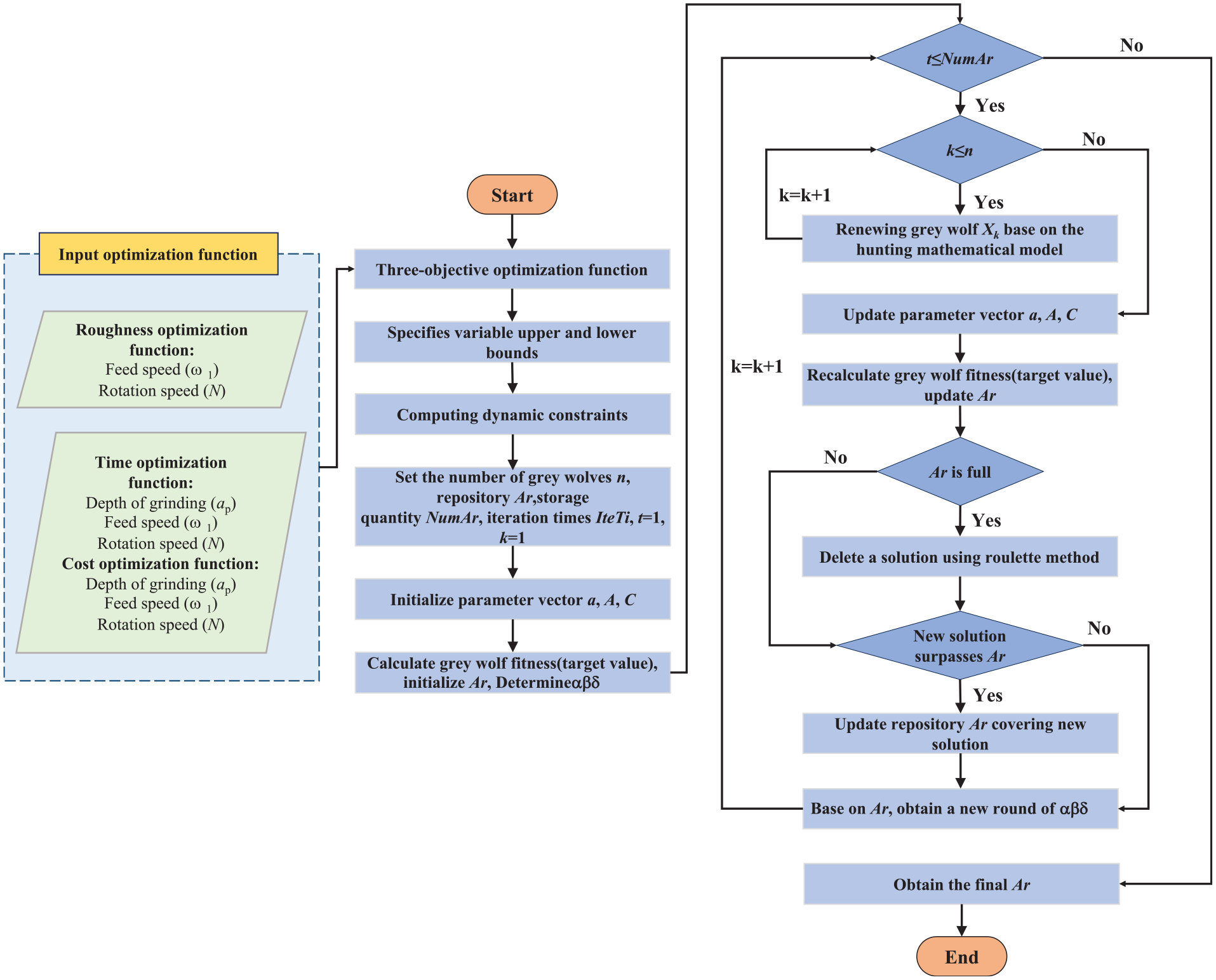
Solution flow chart.

Results and discussion

Analysis of optimization results

In this study, the parameters were set as follows: the maximum number of iterations was 300, the population size was 100, and there were 50 grey wolves per iteration. A test case is used to study the effectiveness of the proposed optimization algorithm with the numerical data listed in Table 5 and the feasible ranges of the variables in Table 6. The Multi-objective Grey Wolf Optimization Algorithm (MOGWO) was utilized to generate a set of Pareto optimal solutions. To evaluate the effectiveness and efficiency of MOGWO, a three-objective function model was also solved using NSGA-II, and the results were compared.

Table 5.

Values of the constants and parameters used in process parameter optimization of grinding process.

Symbol	Definition	Units	Value
$a_{p - min}$	The minimum values of the cutting depth constraint	mm	0.05
$a_{p - max}$	The maximum values of the cutting depth constraint	mm	0.35
C_pl	Cost per unit volume of grinding fluid	$	1
C_d	Total grinding wheel dressing cost	$	10
C_wr	The cost of one treatment of waste residue	$	20
C_s	Unit price of electricity	$	0.2
C _max	The maximum cost constraint	$	10
d ₀	The spindle diameter	mm	950
d_g	Grind size	mm	0.1
Doc	The depth of dressing	mm	0.015
f_d	Cross feed rate	mm/pass	1.2
$F'_{0}$	The grinding force just before sparkout began	N/mm	50
G	The grinding ratio of the grinding wheel	\	142.79
k_w	Price of grinding wheel per unit volume	$	0.04
k_h	Operator hourly rate	$	25
L	The lead of dressing	mm	0.137
L_x	The feed distance on the x-axis	mm	10
L_y	The feed distance on the y-axis	mm	10
m_wr	The quality of waste slag treated at one time	g	100
M _max	The maximum value of the spindle torque constraint	Nm	50
n_D	Number of grinding parts after grinding wheel dressing	\	50
n _min	The minimum values of the speed constraint	rpm	50
n _max	The maximum values of the speed constraint	rpm	250
N _min	The minimum values of the grinding wheel speed constraint	rpm	12,000
N _max	The maximum values of the grinding wheel speed constraint	rpm	25,000
P _e	The rated power of the machine tool	kw	10
Q_w	Material removal rate per unit width	\	0.8
Ra _max	The maximum value of surface roughness constraint	mm	0.5
R_c	Workpiece hardness (Rockwell hardness number)	\	40
t_a	Auxiliary grinding time	s	100
T_cl	Replacement cycle time of grinding fluid	min	28,800
v_xf	The tool withdrawal speed on the x axis	mm/s	5
v_yf	The tool withdrawal speed on the y axis	mm/s	5
V_s	Volume of grinding fluid under a single load	mm³	50
VOL	Wheel bond percentage	%	6.53
ψ	Total rotation angle of worm	°	6π
ρ	Density of workpiece	g/mm³	0.00785
ω _min	The minimum values of worm angular velocity	rad/s	0.01
ω _max	The maximum values of worm angular velocity	rad/s	0.25

Table 6.

The grinding process variables, upper and lower bound.

Grinding parameters	Rotation speed N (rpm)	Feed speed ω₁ (rad s⁻¹)	Depth of grinding a_p (mm)
Range	12,000–25,000	0.01–0.25	0.05–0.35

Table 7 presents the optimization results obtained using NSGA-II alongside those obtained through MOGWO in this study.

Table 7.

Results of NSGA-II and MOGWO in solving tri-objective model of grinding process.

Pareto optimal solution	NSGA-II						MOGWO (this research)
	Decision variables			Objective functions value			Decision variables			Objective functions value
	N	ω ₁	a_p	R _a	C_total	T_total	N	ω ₁	a_p	R _a	C_total	T_total
1	24,548	0.2224	0.1621	0.557	3.8576	192.8299	25,000	0.2093	0.3253	0.5396	4.0640	198.2106
2	24,478	0.1444	0.1533	0.4691	5.2782	238.6084	24,819	0.1510	0.3203	0.4750	5.1414	232.9286
3	24,558	0.1767	0.1495	0.5079	4.5436	214.7599	24,717	0.1746	0.3289	0.5042	4.6006	216.1012
4	24,555	0.1511	0.1493	0.4772	5.1069	232.8063	24,876	0.1825	0.3285	0.5119	4.4691	211.4021
5	24,601	0.1562	0.1422	0.4832	4.9852	228.7349	25,000	0.1697	0.3151	0.4963	4.7282	219.1819
6	24,561	0.1292	0.144	0.4481	5.7679	253.941	25,000	0.0947	0.2953	0.3930	7.5154	307.1861
7	24,589	0.1157	0.1455	0.4286	6.3031	270.9338	24,700	0.1044	0.2974	0.4106	6.8757	288.6647
8	24,632	0.1195	0.1455	0.4338	6.1495	265.8067	24,469	0.1098	0.2899	0.4205	6.5600	279.8351
9	24,495	0.1229	0.145	0.4397	5.9933	261.4736	24,909	0.1453	0.3105	0.4671	5.3081	237.8540
10	24,564	0.1255	0.147	0.4429	5.9047	258.3116	24,389	0.1495	0.3037	0.4764	5.1286	234.2042
11	24,628	0.1937	0.1534	0.5263	4.2576	205.3924	24,682	0.1519	0.3098	0.4772	5.1022	232.2136
12	24,607	0.217	0.1392	0.5511	3.9276	194.9036	24,710	0.1378	0.3018	0.4587	5.5051	244.9371
13	24,551	0.2091	0.1441	0.5434	4.0262	198.2135	24,759	0.1042	0.2916	0.4099	6.8979	289.0362
14	24,494	0.1812	0.1422	0.5137	4.4527	212.0565	24,801	0.1071	0.2995	0.4141	6.7521	284.1704
15	24,638	0.1612	0.1496	0.489	4.8721	224.9841	24,512	0.1513	0.3058	0.4777	5.0982	232.7458
16	24,440	0.1117	0.1433	0.4237	6.4601	276.7424	24,800	0.1454	0.3087	0.4680	5.2913	237.7638
17	24,569	0.1661	0.1438	0.4954	4.7575	221.5672	24,604	0.1509	0.3104	0.4765	5.1189	233.0483
18	24,624	0.1339	0.1413	0.4542	5.6156	248.7886	24,939	0.1454	0.3090	0.4669	5.3095	237.7789
19	24,643	0.2212	0.1295	0.5549	3.8795	193.2689	24,800	0.1565	0.3133	0.4816	5.0071	228.5885
20	24,547	0.1968	0.1487	0.5304	4.2012	203.8323	24,867	0.1528	0.3080	0.4768	5.1027	231.5147
21	24,548	0.187	0.1456	0.5197	4.3585	208.8673	24,913	0.1474	0.3043	0.4697	5.2510	236.0296
22	24,494	0.1898	0.1422	0.5232	4.3073	207.3941	24,900	0.1528	0.308	0.4768	5.1027	231.5147
23	24,533	0.1311	0.1479	0.451	5.698	251.8291	24,940	0.1457	0.3091	0.4674	5.3000	237.4769
24	24,629	0.114	0.1484	0.4258	6.3855	273.3617	24,200	0.1076	0.2951	0.4191	6.6194	283.3113
25	24,525	0.1455	0.1444	0.4703	5.2519	237.5697	24,796	0.1452	0.3035	0.4678	5.2962	237.9308
26	24,484	0.1997	0.1413	0.5341	4.152	202.441	24,868	0.0850	0.2873	0.3771	8.2059	329.8911
27	24,518	0.2049	0.1456	0.5393	4.0807	200.0572	24,600	0.1033	0.2916	0.4093	6.9234	290.5153

Table 7 clearly demonstrates that several Pareto optimal solutions obtained by MOGWO significantly outperform those generated by NSGA-II, indicating superior performance. For instance, MOGWO’s ninth Pareto optimal solution notably dominates a majority of NSGA-II results. While NSGA-II provides trade-offs among objective functions within its Pareto optimal solutions, MOGWO consistently delivers higher-quality solutions termed as efficient Pareto optimal solutions, which cannot be surpassed by others. As depicted in Figure 7(b), while NSGA-II demonstrates good convergence, it may converge to a local optimal solution if the solutions are overly concentrated. On the other hand, MOGWO exhibits a robust feedback mechanism, achieving a balance between local optimization and global search. Figure 7(a) illustrates that MOGWO displays strong search behavior during the process of solving Pareto optimal solutions, thereby offering more reliable candidate solutions and effectively avoiding the pitfalls of local optimal solutions.

Figure 7.

Results of solving Pareto optimal solutions: (a) solution results of MOGWO and (b) solution results of NSGA-II.

Figure 8(a) to (c) display the scatter distribution of the obtained optimal objective function solutions and their centroids. It is evident that the optimized solution set is evenly distributed and of high quality. Figure 8(d) illustrates the distribution and variation trend of the processing parameters within the optimal solution set. The centroid diagrams provide specific ranges for selecting the optimal solutions. It can be observed that the centroid range of T_total is between 230 and 270, the centroid range of C_total is between 5 and 6, and the centroid range of roughness is between 0.43 and 0.48. The centroids of the three objectives all concentrate on the Pareto solutions from the 10th to the 18th group, providing a fundamental range for selecting the optimal solution.

Figure 8.

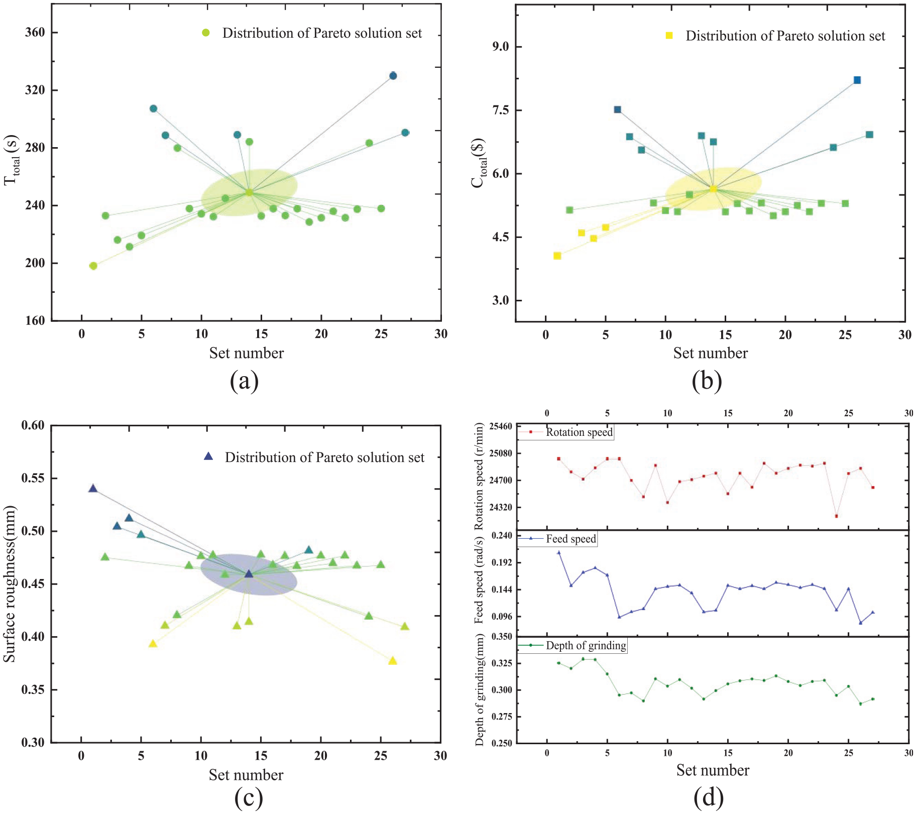
Distribution of optimal solution set for MOGWO: (a) scatter distribution and centroid of machining time, (b) scatter distribution and centroid of processing cost, (c) roughness scatter distribution and scatter centroid, and (d) range of rotation speed, feed speed and depth of grinding.

To screen the Pareto optimal solution set acquired through the MOGWO, the optimal processing parameter combination is selected. The dataset was processed using the Technique for Order Preference by Similarity to an Ideal Solution (TOPSIS), a widely used method for solving Multiple Criteria Decision Making (MCDM) problems. The specific steps adopted in this study are as follows:

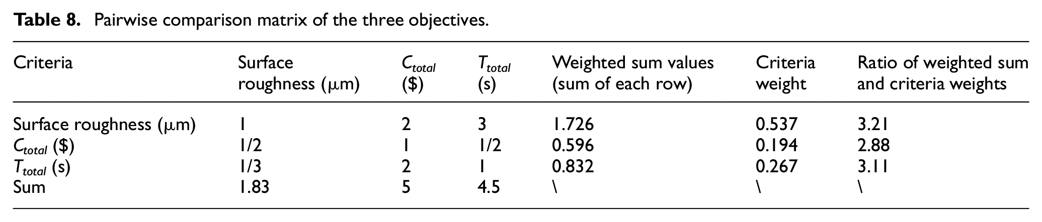
Step 1: The Analytic Hierarchy Process (AHP) proposed by Saaty et al. is used to determine the priority values of different criteria.⁵⁴ The standard weight value of each row is calculated, and the obtained values are: Surface Roughness = 0.537, C_total = 0.194, and T_total = 0.267. The consistency value was determined by multiplying the pairwise matrices with the criteria weights and summing them by columns. This process yielded the ratio of the weighted sum to the criteria weights, as illustrated in Table 8. Then, the average of the consensus value λ_max is calculated as shown in equation (47):

λ_{max} = \frac{3.21 + 2.88 + 3.11}{3} = 3.067 .

(47)

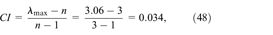
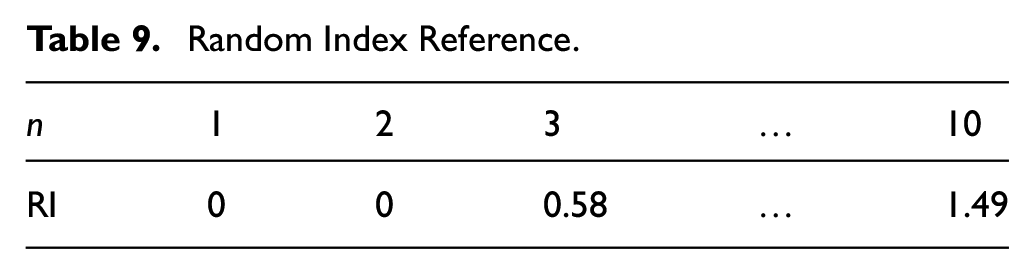
Step 2: Calculate the consistency index CI using equation (48) and then calculate the random consistency index CR via equation (49). Where RI is the random index and 0.58 is selected as the reference value according to Table 9. The comparison indicates that the inconsistency degree of the decision matrix falls within the allowable range, and the consistency test is successfully passed.

CI = \frac{λ_{max} - n}{n - 1} = \frac{3.06 - 3}{3 - 1} = 0.034,

(48)

CR = \frac{CI}{RI} = \frac{0.034}{0.58} = 0.059 < 0.10 .

(49)

Step 3: To obtain the weighted normalized matrix, multiply the standard weights by the output values of each output factor, as depicted in Table 10.

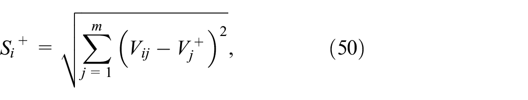
Step 4: Rank the alternatives according to the shortest Euclidean distance (PIS) from the positive ideal solution (PIS) and the longest Euclidean distance from the negative ideal solution (NIS). The positive ideal (best) S_i⁺ and negative ideal (worst) S_i⁻ results were calculated using the following formula, and the relative proximity coefficient C_i for each combination of grinding factors was calculated as shown in Table 11.

{S_{i}}^{+} = \sqrt{\sum_{j = 1}^{m} {(V_{ij} - V_{j}^{+})}^{2}},

(50)

{S_{i}}^{-} = \sqrt{\sum_{j = 1}^{m} {(V_{ij} - V_{j}^{-})}^{2}},

(51)

and

C_{i} = \frac{{S_{i}}^{-}}{{S_{i}}^{+} + {S_{i}}^{-}} .

(52)

Table 8.

Pairwise comparison matrix of the three objectives.

Criteria	Surface roughness (µm)	C_total ($)	T_total (s)	Weighted sum values (sum of each row)	Criteria weight	Ratio of weighted sum and criteria weights
Surface roughness (µm)	1	2	3	1.726	0.537	3.21
C_total ($)	1/2	1	1/2	0.596	0.194	2.88
T_total (s)	1/3	2	1	0.832	0.267	3.11
Sum	1.83	5	4.5	\	\	\

Table 9.

Random Index Reference.

n	1	2	3	…	10
RI	0	0	0.58	…	1.49

Table 10.

Weighted normalized matrix for MOGWO solutions.

Experiment number	Surface roughness (µm)	C_total ($)	T_total (s)
1	0.2898	0.7884	52.9222
2	0.2551	0.9974	62.1919
3	0.2708	0.8925	57.6990
4	0.2749	0.8670	56.4444
5	0.2665	0.9173	58.5216
6	0.2110	1.4580	82.0187
7	0.2205	1.3339	77.0735
8	0.2258	1.2726	74.7160
9	0.2508	1.0298	63.5070
10	0.2558	0.9949	62.5325
11	0.2563	0.9898	62.0010
12	0.2463	1.0680	65.3982
13	0.2201	1.3382	77.1727
14	0.2224	1.3099	75.8735
15	0.2565	0.9891	62.1431
16	0.2513	1.0265	63.4829
17	0.2559	0.9931	62.2239
18	0.2507	1.0300	63.4870
19	0.2586	0.9714	61.0331
20	0.2560	0.9899	61.8144
21	0.2522	1.0187	63.0199
22	0.2560	0.9899	61.8144
23	0.2510	1.0282	63.4063
24	0.2251	1.2842	75.6441
25	0.2512	1.0275	63.5275
26	0.2025	1.5919	88.0809
27	0.2198	1.3431	77.5676

Table 11.

Ideal positive and negative solutions, and relative closeness to the ideal solution of grinding process.

Experiment number	S_i ⁺	S_i ⁻	C_i
1	0.733	0.680	0.4812
2	0.476	0.580	0.5492
3	0.580	0.610	0.5127
4	0.611	0.625	0.5054
5	0.548	0.604	0.5240
6	0.569	0.671	0.5413
7	0.488	0.620	0.5594
8	0.460	0.598	0.5652
9	0.454	0.577	0.5594
10	0.483	0.574	0.5432
11	0.483	0.579	0.5451
12	0.439	0.572	0.5658
13	0.490	0.622	0.5594
14	0.473	0.613	0.5647
15	0.486	0.577	0.5428
16	0.457	0.576	0.5573
17	0.482	0.578	0.5452
18	0.453	0.577	0.5601
19	0.496	0.585	0.5412
20	0.481	0.582	0.5474
21	0.461	0.578	0.5564
22	0.481	0.582	0.5474
23	0.455	0.577	0.5594
24	0.471	0.598	0.5594
25	0.457	0.575	0.5574
26	0.680	0.733	0.5188
27	0.495	0.623	0.5570

This paper introduces a constraint model based on dynamic variations in grinding ratio and machining stiffness. This model effectively regulates optimization outcomes, ensuring parameter combinations align closely with real-world machining conditions. Furthermore, to manage technological costs, parameter ranges are tailored to existing processing conditions. This strategic approach confines MOGWO’s optimization scope, preventing significant deviations in processing factors. As depicted in Table 11, the comprehensive score C_i of Pareto optimal solutions obtained by TOPSIS is relatively close. Nevertheless, due to its non-gradient mechanism, adaptive parameter adjustment, and flexibility, MOGWO exhibits robust convergence across various processing ranges. It can select the collocation combination with practical reference significance.

Figure 9 indicates that the TOPSIS score is consistently high with minimal change, signifying the ideal optimization result achieved by MOGWO. In this study, the highest score serves as the final optimization result, as detailed in Table 12. By comparing the results of the three objective optimizations, it becomes apparent that time and cost exhibit similar trends, with the processing cost objective function closely proportional to the time function. Within the chosen parameter range, the variability in processing cost is minimal. However, due to factors like weight and change amount, the substantial variation in processing time notably impacts the roughness model. Therefore, optimizing processing time alongside processing quality holds significant practical importance in real-world processing scenarios. The optimization results shown in Table 12 indicates that the processing cost adheres to the constraints, while both processing time and surface roughness undergo significant reductions.

Figure 9.

The Pareto front showing the tradeoff between roughness, cost, and time.

Table 12.

Experimental comparison of optimization results.

Optimization parameters	Optimal design
	Before optimization	After optimization
Rotation speed N (rpm)	16,000	24,710
Feed speed ω₁ (rad s⁻¹)	0.1	0.1378
Depth of grinding a_p (mm)	0.1	0.3018
Surface roughness (µm)	0.4801	0.4587
C_total ($)	5.5222	5.5051
T_total (s)	296.5756	244.9371

To facilitate a direct analysis of the differences in optimization results, the outcomes are normalized for comparison, as shown in Figure 10. Table 12 and Figure 10 collectively demonstrate that the MOGWO algorithm significantly enhances the optimization objectives compared to conventional parameters. Particularly noteworthy is the comparison with commonly used grinding process parameters, wherein the optimized grinding time is reduced by 17.41%, surface quality improves by 4.46%, and grinding cost decreases by 1.12%. This substantiates the feasibility and practicality of the method.

Figure 10

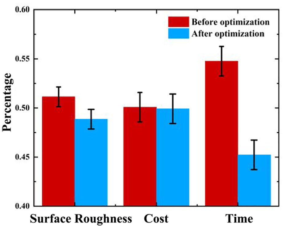
Comparison of optimization results.

Analysis of different worm transmission coefficients

The REWR exhibits varying specifications and sizes across different application scenarios. To assess the adaptability of the optimization model, Table 13 presents three sets of different transmission coefficient combinations based on common size specifications for comparative analysis.

Table 13.

Optimization results for different transmission coefficient combinations.

Worm parameter	Small	Regular	Large
Center distance A (mm)	53	63	73
Roller radius R (mm)	4	5	6
Transmission ratio i₂₁	25	20	23
Rotation speed N (rpm)	16,000	16,000	16,000
Feed speed ω₁ (rad s⁻¹)	0.08	0.1	0.12
Depth of grinding a_p (mm)	0.05	0.1	0.15

Worm manufacturing in diverse operational scenarios often involves varying sizes. To validate the effectiveness of the proposed optimization model, three sets of commonly used size specifications are compared and analyzed. Table 14 delineates the range of processing parameters. As the overall processing size decreases, there is an increased demand for processing accuracy and other aspects, necessitating more stringent control requirements for processing quality. Conversely, the larger size of the large Roller Enveloping Worm Reducer (REWR) surface grinding affords enhanced overall stiffness and stability, thereby facilitating better control over processing quality. Figure 11 illustrates the optimization results for the three sets of commonly used specifications. The Pareto solution set is evaluated using TOPSIS screening, and the optimal solution is selected and normalized for comparison. The proposed three-objective optimization function demonstrates excellent adaptability across various processing scenarios, as observed in the optimization of parameter combinations with reference values using MOGWO. Significant enhancements in processing efficiency are evident after optimizing various transmission coefficients. However, as size increases and material removal volume grows, cost control becomes more challenging. Therefore, MOGWO not only greatly improves processing efficiency and surface quality but also endeavors to control costs as much as possible. When designing machining parameters, considerations such as load-bearing capacity, size constraints, and machining precision must be balanced comprehensively. Optimization of these three objectives is crucial for achieving optimal outcomes.

Table 14.

Grinding process variables with different transmission coefficients, upper and lower bounds.

Size	Rotation speed N (rpm)	Feed speed ω₁ (rad s⁻¹)	Depth of grinding a_p (mm)
Small	12,000–22,000	0.01–0.25	0.01–0.30
Regular	12,000–25,000	0.01–0.25	0.05–0.35
Large	12,000–26,000	0.01–0.25	0.05–0.35

Figure 11.

Comparison of optimization results of different transmission coefficients: (a) center distance is 53 mm, roller radius is 4 mm, and transmission ratio is 25, (b) center distance is 63 mm, roller radius is 7 mm, and transmission ratio is 20, and (c) center distance is 73 mm, roller radius is 6 mm, and transmission ratio is 23.

Conclusion

This paper investigates challenging combinatorial optimization problems in complex surface machining processes, such as roller enveloping worms, focusing on optimizing surface quality, machining time, and cost while adhering to predefined constraints. The specific innovation points are reflected in the following aspects:

We leveraged the geometric and kinematic mechanisms governing worm tooth surface grinding by the grinding wheel to establish a predictive model for tooth surface roughness. Drawing from real-world machining processes, we developed a predictive model for machining time and cost, specifically tailored for complex surfaces, and integrated it with a prediction model for surface roughness. Experimental validation confirmed the effectiveness of our model, providing a robust basis for multi-objective optimization.

For the unique machining surface under study, we devised a grinding ratio constraint model incorporating the improvement workpiece removal parameter (IWRP) and improvement wheel wear parameter (IWWP). To mitigate the risk of tooth surface quality degradation due to machine tool chatter, we introduced improvement grinding stiffness (IK_c) and improvement wheel wear stiffness (IK_s) to establish a machining stiffness constraint model. The feasible region of the specification solution increases the reality of the optimization function.

The Multi-objective Grey Wolf Optimization Algorithm (MOGWO) decision model is utilized to optimize the three objective functions and produce a set of non-dominated Pareto optimal solutions, providing technicians with a parameter selection space. The results of the MOGWO analysis demonstrate good feasibility across all cases.

In light of the inherent conflict between achieving tooth surface roughness and the other two objectives, we employ the Analytic Hierarchy Process (AHP) method to balance the three objectives and determine the optimal weight allocation for optimization. Subsequently, we utilize the TOPSIS evaluation system to assess the obtained optimal solution set, providing a combination of optimal Pareto solutions. Verification has demonstrated that this combination optimizes surface quality, processing time, and processing cost holistically.

Footnotes

Handling Editor: Divyam Semwal

Author contributions

Jiongkang Ren: Conceptualization, Methodology, Investigation, Software, Validation, Data curation, Writing-original draft, Visualization. Shisong Wang: Methodology, Writing-review & editing, Visualization. Keqi Ren: Methodology, Software, Data curation.

Declaration of conflicting interests

The author(s) declared no potential conflicts of interest with respect to the research, authorship, and/or publication of this article.

Funding

The author(s) disclosed receipt of the following financial support for the research, authorship, and/or publication of this article: This work was supported by the National Natural Science Foundation of China (Nos. U23A20619 and 52175039) and the Chengdu Municipal Science and Technology Program (2023-JB00-00024-GX). The authors would also like to thank the support from Sichuan CNC Equipment Ultra-Precision Drive and Transmission Engineering Research Center and Chengdu Zhongliang Chuangong Technology Co., Ltd.

Ethics approval

The article follows the guidelines of the Committee on Publication Ethics (COPE) and involves no studies on human or animal subjects.

Data availability statement

The authors state that all the data necessary to replicate the results are presented in the manuscript. Relevant parts of the code can be shared by contacting the corresponding author.

ORCID iD

Jiongkang Ren

References

Meng

Guo

Zhao

, et al. Modelling of grinding mechanics: a review. Chin J Aeronaut 2022; 36: 25–39.

Deng

. Study on the zero-backlash roller enveloping precision reducer. Singapore: Springer, 2022.

Deng

Wang

, et al. Investigation on the backlash of roller enveloping hourglass worm gear: theoretical analysis and experiment. J Mech Des 2019; 141: 053302.

Deng

Wang

, et al. Theory and experiment study of anti-backlash single- and double-roller enveloping hourglass worm gear. Chin J Mech 2020; 56: 88–95.

Wang

Zhang

, et al. Assessment and optimization of grinding process on AISI 1045 steel in terms of green manufacturing using orthogonal experimental design and grey relational analysis. J Clean Prod 2020; 253: 119896.

Dražumerič

Badger

Roininen

, et al. On geometry and kinematics of abrasive processes: the theory of aggressiveness. Int J Mach Tools Manuf 2020; 154: 103567.

Setti

Arrabiyeh

Kirsch

, et al. Analytical and experimental investigations on the mechanisms of surface generation in micro grinding. Int J Mach Tools Manuf 2020; 149: 103489.

Guo

, et al. Three-dimensional topography modelling and grinding performance evaluating of micro-structured CVD diamond grinding wheel. Int J Mech Sci 2023; 244: 108079.

Zhang

Huo

Zhang

, et al. Fabrication and size prediction of crystalline nanoparticles of silicon induced by nanogrinding with ultrafine diamond grits. Scr Mater 2012; 67: 657–660.

10.

Zhang

Song

, et al. A novel model for undeformed nanometer chips of soft-brittle HgCdTe films induced by ultrafine diamond grits. Scr Mater 2012; 67: 197–200.

11.

Zhang

Wang

Kang

, et al. Changes in surface layer of silicon wafers from diamond scratching. CIRP Ann Manuf Technol 2015; 64: 349–352.

12.

Wang

Zhang

Chang

, et al. New deformation-induced nanostructure in silicon. Nano Lett 2018; 18: 4611–4617.

13.

Zhang

Cui

Wang

, et al. A novel approach of mechanical chemical grinding. J Alloys Compd 2017; 726: 514–524.

14.

Gao

Wang

, et al. Theoretical prediction and sensitivity analysis of surface roughness of abrasive belt grinding. Surf Technol 2018; 47: 295–305. (in Chinese)

15.

Wang

Zhao

. Optimization of gear grinding parameters with worm grinding wheel. Chin J Mech Eng 2021; 32: 2136–2141. (in Chinese)

16.

Wen

Tay

AAO

Nee

AYC

. Micro-computer-based optimization of the surface grinding process. J Mater Process Technol 1992; 29: 75–90.

17.

Baskar

Saravanan

Asokan

, et al. Ants colony algorithm approach for multi-objective optimization of surface grinding operations. Int J Adv Manuf Technol 2004; 23: 311–317.

18.

Krishna

. Optimization of surface grinding operations using a differential evolution approach. J Mater Process Technol 2007; 183: 202–209.

19.

Krishna

Rao

. Multi-objective optimization of surface grinding operations using scatter search approach. Int J Adv Manuf Technol 2006; 29: 475–480.

20.

Lee

Hsu

Chou

, et al. Improved differential evolution approach for optimization of surface grinding process. Expert Syst Appl 2011; 38: 5680–5686.

21.

Lin

. Enhanced Pareto particle swarm approach for multi-objective optimization of surface grinding process. In: 2008 second international symposium on intelligent information technology application, Shanghai, China, 20–22 December 2008, pp.618–623. New York: IEEE.

22.

Cui

Geng

Zhu

, et al. Review: multi-objective optimization methods and application in energy saving. Energy 2017; 125: 681–704.

23.

Gholami

Azizi

. Constrained grinding optimization for time, cost, and surface roughness using NSGA-II. Int J Adv Manuf Technol 2014; 73: 981–988.

24.

Jiang

Xiao

, et al. A multi-objective modeling and optimization method for high efficiency, low energy, and economy. Int J Adv Manuf Technol 2023; 128: 2483–2498.

25.

Pawar

Rao

Davim

. Multi-objective optimization of grinding process parameters using particle swarm optimization algorithm. Mater Manuf Process 2010; 25: 424–431.

26.

Huang

Zhao

Qiu

, et al. MOPSO process parameter optimization in ultrasonic vibration-assisted grinding of hardened steel. Int J Adv Manuf Technol 2023; 128: 903–914.

27.

Liu

. Application of ant colony optimization algorithm in process planning optimization. J Intell Manuf 2013; 24: 1–13.

28.

Alajmi

Alfares

. Selection of optimal conditions in the surface grinding process using the quantum based optimization method. J Intell Manuf 2019; 30: 1469–1481.

29.

Khalilpourazari

Khalilpourazary

. Optimization of time, cost and surface roughness in grinding process using a robust multi-objective dragonfly algorithm. Neural Comput Appl 2020; 32: 3987–3998.

30.

Shehab

Khader

Al-Betar

. A survey on applications and variants of the cuckoo search algorithm. Appl Soft Comput 2017; 61: 1041–1059.

31.

Saxena

Soni

Kumar

, et al. Intelligent grey wolf optimizer - development and application for strategic bidding in uniform price spot energy market. Appl Soft Comput 2018; 69: 1–13.

32.

Gao

Pan

, et al. A multi-objective cellular grey wolf optimizer for hybrid flowshop scheduling problem considering noise pollution. Appl Soft Comput 2019; 75: 728–749.

33.

Wang

Ren

, et al. Roughness prediction model of worm with a complicated space surface under grinding. J Manuf Process 2024; 126: 332–347.

34.

Ono

Kawamura

Kitano

, et al. Cutting theories. 1st ed. Beijing: National Defense Industry Press, 1985.

35.

Zhu

, et al. Surface roughness prediction model of SiCp/Al composite in grinding. Int J Mech Sci 2019; 155: 98–109.

36.

Wang

Chen

Zhou

, et al. Roughness model for tooth surfaces of spiral bevel gears under grinding. Mech Mach Theory 2016; 104: 17–30.

37.

Wang

Liu

Chu

, et al. Calculation model for surface roughness of face gears by disc wheel grinding. Int J Mach Tools Manuf 2017; 123: 76–88.

38.

Yuan

Han

Wang

, et al. Modeling and analysis of tooth surface roughness for internal gearing power honing gear. J Braz Soc Mech Sci Eng 2017; 39: 3607–3620.

39.

Liu

Huang

Cao

, et al. Model of surface texture for honed gear considering motion path and geometrical shape of abrasive particle. Chin J Mech Eng 2023; 36: 311–325.

40.

Xiu

Cai

. Modification for theoretical model of ground surface roughness. J Northeast Univ Nat Sci 2005; 26: 770–773. (in Chinese)

41.

Wegener

Hoffmeister

Karpuschewski

, et al. Conditioning and monitoring of grinding wheels. CIRP Ann Manuf Technol 2011; 60: 757–777.

42.

Witzendorff

Stompe

Moalem

, et al. Dicing of hard and brittle materials with on-machine laser-dressed metal-bonded diamondblades. Precis Eng 2014; 38: 162–167.

43.

King

Hahn

. Handbook of modern grinding technology. London: Chapman and Hall, 1986.

44.

Malkin

. Grinding technology: theory and applications of machining with abrasives. New York, NY: Industrial Press Inc, 2008.

45.

Deng

Zhang

, et al. Optimization of process parameters for minimum energy consumption based on cutting specific energy consumption. J Clean Prod 2017; 166: 1407–1414.

46.

Brendon

. Depreciation and the time value of money. arXiv preprint arXiv:1605.00080, 2016.

47.

Mirjalili

Lewis

. Grey wolf optimizer. Adv Eng Softw 2014; 69: 46–61.

48.

Mirjalili

Saremi

Mirjalili

S M

, et al. Multi - objective grey wolf optimizer: a novel algorithm for multi-criterion optimization. Expert Syst Appl 2016; 47: 106–119.

49.

Coello

CAC

Pulido

Lechuga

. Handling multiple objectives with particle swarm optimization. IEEE Trans Evol Comput 2004; 8: 256–279.

50.

Deb

Pratap

Agarwal

, et al. A fast and elitist multi-objective genetic algorithm: NSGA-II. IEEE Trans Evol Comput 2002; 6: 182–197.

51.

Knowles

Corne

. The Pareto archived evolution strategy: a new baseline algorithm for Pareto multi-objective optimization. In: Proceedings of the 1999 congress on evolutionary computation-CEC99, Washington, DC, USA, 6–9 July 1999, pp.98–105. New York: IEEE.

52.

Srinivas

Deb

. Multi-objective optimization using nondominated sorting in genetic algorithms. Evol Comput 1994; 2: 221–248.

53.

Zitzler

Thiele

Multi-objective optimization using evolutionary algorithms - a comparative case study. In: Eiben

Bäck

Schoenauer

, et al. (eds) Parallel problem solving from nature. Berlin, Heidelberg: Springer, 1998, pp.292–301.

54.

Saaty

Vargas

. Estimating technological coefficients by the analytic hierarchy process. Socioecon Plann Sci 1979; 13: 333–336.

Multi-objective optimization of grinding process parameters for complicated worm space surface based on the grey wolf optimization algorithm

Abstract

Keywords

Introduction

Optimization model of tooth surface grinding

Modeling of grinding roughness

Modeling of machining time

No-load time

Material removal time

Other auxiliary time

Modeling of machining cost

Grinding fluid consumption cost

Grinding wheel cost

Waste disposal cost

Energy cost of grinding process

Equipment usage cost

Labor cost

Experimental setup

Multi-objective optimization of worm grinding

Constraint setting

Processing condition constraints

Grinding ratio constraint

Machining stiffness constraints

Multi-objective Grey Wolf optimization algorithm

Encircling prey

Search for prey (exploration)

Results and discussion

Analysis of optimization results

Analysis of different worm transmission coefficients

Conclusion

Footnotes

Author contributions

Declaration of conflicting interests

Funding

Ethics approval

Data availability statement

ORCID iD

References