Multi-physical modeling and analysis on UAV launching system

Abstract

For UAVs unable to take off vertically, a launch device is essential, and accurate launch velocity prediction is crucial. This study develops two mathematical models for both the mechanical and the pneumatic subsystems of the launching system of unmanned aerial vehicles (UAVs) and solves these coupled, highly nonlinear ordinary differential equations by the fourth-order Runge-Kutta method. By applying this multi-physical model to the launching systems of UAVs, the trend with time of the shuttle displacement, velocity, and acceleration, as well as the tank and cylinder pressures in the mathematical results, are similar to those observed in real experiments. Using MATLAB as the platform, this multi-physical model accurately predicts the velocity of the launching system (or dummy), with a maximum error of 9.0% and a minimum error of 4.3% compared to the experimental results. Additionally, this multi-physical model reveals a linear relationship between the frictional force and pull force of the shuttle, which is consistent with the co-simulation results. Overall, these models not only offer the greatest design flexibility to understand and meet the required launching system’s performance, it will also save the cost and time for the efficient R&D procedure of future UAVs’ applications.

Introduction

Unmanned aerial vehicles (UAVs) encompass a diverse range of remote-controlled aircraft that operate autonomously, eliminating the need for onboard pilots. The components of UAV systems typically comprise a control station, payload, air vehicle, navigation system, launching system, recovery system, support equipment, and transportation. ¹ This study mainly focuses on the launch device. Usually, UAVs that cannot take-offs vertically or do not have landing gear require a launch device. Launching systems become essential for their deployment.

Francis, ² Novaković and Medar ³ employed the quality function deployment (QFD) approach to develop quantifiable engineering specifications to meet customer needs. Among the essential requirements identified by customers, the final launch velocity and the capacity to launch mass were deemed crucial. According to research conducted by Novaković and Medar, ³ the most critical aspect in the research and development of launching systems is ensuring that the maximum launching velocity exceeds the stall velocity of the UAV. Additionally, Novaković and Medar ³ suggested that the launching systems’ launching velocity should be at least 15% higher than the stall velocity to ensure safe UAV launches. Therefore, accurately predicting the launching systems’ launching velocity is paramount. The launching velocity of pneumatic launching systems relies on the pressure differential and the mass flow rate of the pneumatic cylinder. Richer and Hurmuzlu ⁴ advocated pneumatic cylinders as superior to electrical or hydraulic actuators. They developed a mathematical model that characterizes bidirectional pneumatic actuators, allowing for precise predictions of the relationship between pressure differential and mass flow rate within the pneumatic cylinder. Thorncroft et al. ⁵ employed the principle of conservation of mass to develop a mathematical model, which they utilized to forecast the correlation between pressure and mass flow rate at the throat of the tank throughout the charging and discharging phases. However, Richer and Hurmuzlu ⁴ and Thorncroft et al. ⁵ focus on a nonlinear model for pneumatic force actuators but overlooks fluid dynamic effects, leading to reduced accuracy in high-speed or high-pressure conditions. In contrast, our study incorporates fluid dynamics, providing a more detailed description of airflow variations on actuator performance, resulting in more accurate dynamic response predictions in practical applications. Siddiqui et al. ⁶ believe the Matlab/Simscape can be used reliably to size the pneumatic launching system. They proposed that the simulation error in tank discharge is 4%, and the whole system’s error is within 8%, when they used the Matlab/Simscape to simulate the performance of the UAV Factory’s 6 KJ pneumatic launching system.

The co-simulation method has emerged as a recent trend, extensively employed to comprehend dynamic phenomena and their impacts. Currently, very limited literature discusses UAV pneumatic launching systems, so there is a lack of comprehensive references to discuss launching systems using the co-simulation method. Regarding the study of the pneumatic launching system, Lee et al. ⁷ conducted a thorough analysis of the velocity performance of the PL-40 launching system using the co-simulation method with Adams and Hypneu. In their study, the results of co-simulation analysis, when compared with realistic launching experiments of a 10 kg dummy launched at 10 bar air tank pressure, showed a velocity error of 3.7%.

A study by Francis, ² Novaković and Medar, ³ and Siddiqui et al. ⁶ revealed that the frictional force between the shuttle and the rail was solely attributed to the normal force exerted by the masses of the UAV and the shuttle from the gravity. However, these studies were limited in scope, primarily focusing on static analysis. The derivation of the shuttle’s kinetics model in Lee et al. ⁷ ’s study points out that the frictional force of the shuttle’s kinetics model is proportional to the pull force during the process of launching the dummy. The results of co-simulation analysis using Adams and Hypneu in Lee et al. ⁷ ’s study also prove that the frictional force between the shuttle and rail is proportional to the pull force of the shuttle. The relationship between frictional force and pull force is linear, contrary to the content proposed in Francis, ² Novaković and Medar, ³ and Siddiqui et al. ⁶ ’s study, where frictional force only considers the normal force generated by the weight of the UAV and shuttle from the gravity. The co-simulation results by Lee et al. ⁷ indicate that considering only the friction force generated by gravity on the mass can lead to a velocity error of up to 7.5%.

Co-simulation method applies multiple independent software or tools, which can couple different physical domains simultaneously through data exchange or interfaces to consider the interactions between mechanisms and pneumatic systems and account for mutual influences between various systems. This approach can yield results closer to real physical phenomena. In Lee et al. ⁷ ’s study, although co-simulation produced satisfactory results, obtaining and using these independent software tools is not easy, and the software for co-simulation is expensive. Therefore, if a multi-physical mathematical model can be developed to communicate with two different physical domains and consider their interactions to produce results close to those of co-simulation, it would greatly benefit the research in relevant fields.

The primary purpose of this study is to develop a multi-physical mathematical model to correctly predict the kinematics of the launching system. The tools required for solving the mathematical model can include any software capable of solving equations, such as C language, MATLAB, LabVIEW, etc. In this study, MATLAB is used. The velocity of the dummy is compared with the realistic launching tests in Lee et al. ⁷ ’s study to verify the reliability and predictability of this multi-physical mathematical model. The frictional force and the pulling force on the shuttle are compared with the co-simulation results in Lee et al. ⁷ ’s study to verify the linear relationship between the frictional force and the pulling force.

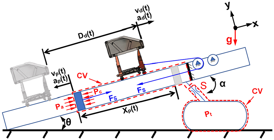
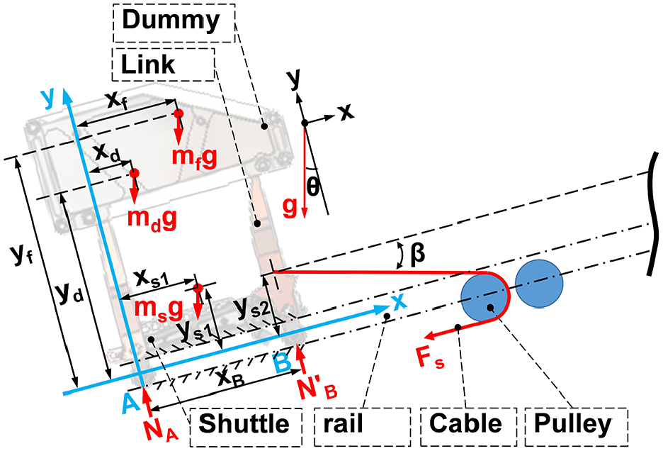
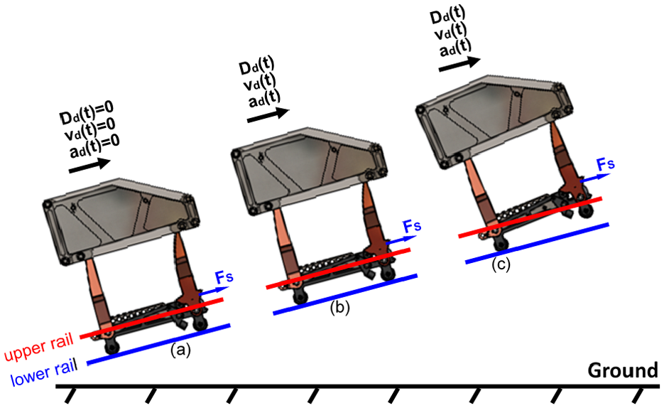
In this research, the target of the study is the pneumatic launching system PL-40, developed by the Estonian company Eli, ⁸ as shown in Figure 1. According to the test data provided by Eli, the PL-40 is capable of launching a 45 kg UAV to a maximum launch velocity of 15.9 m/s and a 10 kg UAV to a maximum velocity of 26.1 m/s. The components of the launching system are shown in the 3D structure of the PL-40, designed using SolidWorks, as shown in Figure 1. In Lee et al. ⁷ ’s study, the UAV was replaced by a dummy, and the launching process is divided into three stages in this paper. The first stage involves moving the shuttle to the initial launch position and assembling the dummy on the shuttle. The second stage is the acceleration process of the shuttle and dummy until the tank pressure is charged to the appropriate pressure. The third stage depicts the separation of the dummy from the shuttle, as shown in Figure 2.

Figure 1.

ELI PL-40 launching system.^7,8

Figure 2.

A schematic depiction shows the launching system and its position at three distinct moments. ⁷

Modeling of launching system

Flow chart for computing and analyzing Multi-physical model

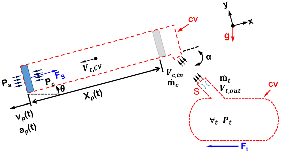
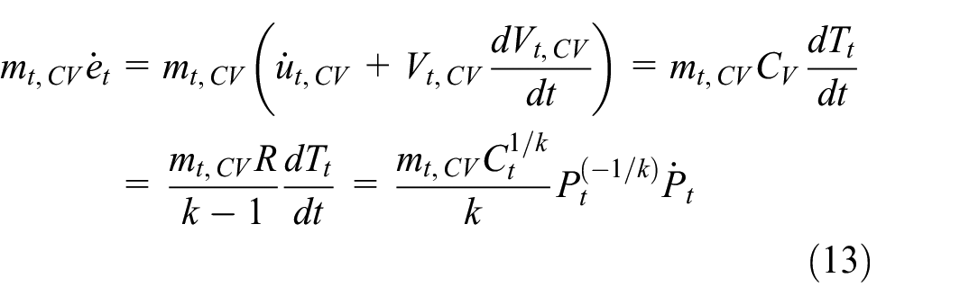
The multi-physical system includes the mechanical and pneumatic power sub-systems. The interaction between the mechanical and pneumatic power systems is shown in Figure 3. Firstly, the equations for the mechanical and pneumatic power systems models must be derived based on the actual operation of the PL-40 launching system. The equations of these two nonlinear coupled mathematical models are programmed and solved based on the platform of Matlab using the 4th-order Runge-Kutta method. The fourth-order Runge-Kutta method is based on high-order Taylor series expansion, which not only achieves high-order truncation error O(h ⁴ ), but also eliminates the calculation of all derivatives, and can obtain more accurate results. The thrust force $F_s(\mathrm{t})$ of the shuttle obtained from the cylinder of the pneumatic power system is outputted to the pneumatic cylinder piston and thus serves as the input condition to the mechanical system via the cable. The results calculated by the mechanical system, including the displacement $D_d(\mathrm{t})$ and velocity $V_d(\mathrm{t})$ of the shuttle, are feedback to the pneumatic cylinder piston via the cable. This iterative calculation repeats itself for each time step until the shuttle reaches the maximum acceleration length $L_d$ of the rail, at which point the iteration stops. After the iteration stops, we compare the dummy velocity with the experimental results in Lee et al. ⁷ Refer to Siddiqui et al. ⁶ ’s study, the acceptable error range for the dummy velocity is set to 10%. If the error of the dummy velocity exceeds 10%, the coefficient of kinetic friction in the model between the wheel and rail and the effective area of the valve will be adjusted; otherwise, the iteration will be stopped. The flow chart of computing and analyzing the multi-physical system is shown in Figure 4.

Figure 3.

The schematic diagram illustrates the interaction between the mechanical and pneumatic power systems. ⁷

Figure 4.

The flow chart of computing and analyzing the multi-physical model.

Pneumatic power system

The pneumatic power system includes (a) a tank of fixed volume and (b) a cylinder with a moving piston that connects the mechanical system via a cable.

Some basic assumptions are made for the tank and the cylinder: (1) compressible fluid, (2) Ideal gas, (3) adiabatic expansion process, (4) no head loss and minor loss, (5) uniform properties inside and across the inlet and outlet; (6) the tank volume is constant and large enough, the fluid motion inside the tank is small and random during the expansion process, (7) neglect the body force, (8) The cable, connecting the piston and the shuttle, is assumed rigid, and the cable’s area can be neglect, (9) the potential energy (gZ) are small and nearly unchanged with time.

The air tank exhausts the air to the cylinder, as shown in Figure 5. The tank is considered upstream, and the cylinder is considered downstream. The subscripts “t” and “c” in this paragraph denote the tank and cylinder, respectively. The subscripts “in” and “out” represent the states of the inlet and outlet of the control volume (CV) tank and cylinder. S indicates the effect area of the valve.

Figure 5.

The air tank exhausted air to the cylinder.

When $P_c/P_t>0.528=\mathrm{B}$ , the flow is not choked. The mass flow rate through the convergent nozzle of the tank is shown in equation (1), and the velocity at the nozzle is shown in equation (2).

$${\stackrel{·}{m}}_t=\frac{P_{t}S}{\sqrt{R{T}_t}}\sqrt{\frac{2k}{(k-1)}}{[{\left(\frac{P_c}{P_t}\right)}^{2/k}-{\left(\frac{P_c}{P_t}\right)}^{(k+1)/k}]}^{1/2}$$

(1)

$$V_{t,\mathrm{out}}=\sqrt{\frac{2\mathrm{kR}{T}_t}{(k-1)}}{[1-{\left(\frac{P_c}{P_t}\right)}^{(k-1)/k}]}^{1/2}$$

(2)

When $P_c/P_t\le 0.528=\mathrm{B}$ , the flow is choked, and the Mach number $M_a=1,k=1.4,\mathrm{and}$ the mass flow rate through the convergent nozzle of the tank is shown in equation (3), and the velocity at the nozzle is shown in equation (4).

$${\stackrel{·}{m}}_t=\frac{P_{t}S}{\sqrt{R{T}_t}}\sqrt{\frac{2k}{(k-1)}}{[{\left(B\right)}^{2/k}-{\left(B\right)}^{(k+1)/k}]}^{1/2}$$

(3)

$$V_{t,\mathrm{out}}=\sqrt{\mathrm{kR}{T}_t}$$

(4)

Mathematical model of tank

Mass conservation

As is depicted in Figure 5, consider a fixed control volume (CV) enclosing the whole tank and no inlet to the tank, namely, ${\stackrel{·}{m}}_{t,\mathrm{in}}=0$ . Thus, the general form of mass conservation gives the relation in equation (5).

$$\frac{d}{\mathrm{dt}}\left(m_{t,\mathrm{CV}}\right)={\stackrel{·}{m}}_{t,\mathrm{CV}}=-{\stackrel{·}{m}}_{t,\mathrm{out}}=-{\stackrel{·}{m}}_t$$

(5)

Linear momentum conservation

As depicted in Figure 5, the general form of the linear momentum equation in the direction of outflow at the tank is shown in equation (6).

$$\begin{array}{c}{F}_t\cos (\alpha -\theta )+(P_t-P_c)S=\frac{d}{\mathrm{dt}}\left(V_{t,\mathrm{CV}}{m}_{t,\mathrm{CV}}\right)\hfill \\ +{\stackrel{·}{m}}_t{V}_{t,\mathrm{out}}={\stackrel{·}{m}}_{t,\mathrm{CV}}{V}_{t,\mathrm{CV}}+m_{t,\mathrm{CV}}{a}_{t,\mathrm{CV}}+{\stackrel{·}{m}}_t{V}_{t,\mathrm{out}}\hfill \end{array}$$

(6)

$P_t$ and $P_c$ represent the absolute pressures inside the tank and the cylinder, respectively. S denotes the nozzle area at the exit of the tank. $F_t$ is the force that holds the tank at a fixed position.

Based on the assumption (6), there is no unified direction of fluid motion except near the exit. Thus, $V_{t,\mathrm{CV}}$ and $a_{t,\mathrm{CV}}$ are nearly zero, and equation (6) will be simplified as equation (7).

$$F_t\cos (\alpha -\theta )+(P_t-P_c)S={\stackrel{·}{m}}_t{V}_{t,\mathrm{out}}$$

(7)

Energy conservation

The general form of energy conservation is shown in equation (8).

$${\stackrel{·}{Q}}_{\mathrm{CV}}=\frac{\partial }{\partial t}\underset{\mathrm{CV}}{\int }e\rho d\forall +\underset{\mathrm{CS}}{\int }(e+P\nu )\rho \overrightarrow{V}d\overrightarrow{A}+{\stackrel{·}{W}}_{\mathrm{CV}}$$

(8)

By definition, $e=u+\mathrm{gZ}+\frac{1}{2}{V}^2$ where u is the specific internal energy, $\mathrm{gZ}$ is the specific potential energy, $\frac{1}{2}{V}^2$ is the specific kinetic energy and v is the specific volume (=1/ρ), respectively. ${\stackrel{·}{Q}}_{\mathrm{CV}}$ is the heat transfer from or into the tank. ${\stackrel{·}{Q}}_{\mathrm{CV}}>0$ denotes the heat transfer added into the tank and vice versa; while ${\stackrel{·}{W}}_{\mathrm{CV}}>0$ is the work done to the environment, and ${\stackrel{·}{W}}_{\mathrm{CV}}<0$ represents the work done by the surroundings to the tank.

The first term of equation (8) is expressed as equation (9).

$$\frac{\partial }{\partial t}\underset{\mathrm{CV}}{\int }e\rho d\forall =\frac{d}{\mathrm{dt}}{\left(\mathrm{em}\right)}_{t,\mathrm{CV}}=m_{t,\mathrm{CV}}{\stackrel{·}{e}}_t+{\stackrel{·}{m}}_{t,\mathrm{CV}}{e}_t$$

(9)

The second term on the right-hand side (RHS) of equation (8) can be expanded to equation (10).

$$\begin{array}{c}\multicolumn{1}{c}{{\int }_{\mathrm{CS}}(e+P\nu )\rho \overrightarrow{V}d\overrightarrow{A}={\stackrel{·}{m}}_t{(e+P\nu )}_{t,\mathrm{out}}-{\stackrel{·}{m}}_{t,\mathrm{in}}{(e+P\nu )}_{t,\mathrm{in}}}\\ ={\stackrel{·}{m}}_t{(e+P\nu )}_{t,\mathrm{out}}\hfill \end{array}$$

(10)

In equation (7), $F_t$ is the force that holds the tank at fixed position; thus no work will be done by this force. However, the term $(P_t-P_c)S$ denotes the net force acting at the exit of the tank. Thus, the work done by this force will be $(P_t-P_c)S{V}_{t,\mathrm{out}}$ .

Also, the tank volume is fixed, or ${\stackrel{·}{\forall }}_t=0$ . Thus, the total work on the RHS of equation (8) can be expanded as equation (11)

$$\begin{array}{c}\multicolumn{1}{c}{{\stackrel{·}{W}}_{\mathrm{CV}}={\stackrel{·}{W}}_t=(\stackrel{·}{P}\forall {)}_t+(P\stackrel{·}{\forall }{)}_t+(P_t-P_c)S{V}_{t,\mathrm{out}}}\\ ={\stackrel{·}{P}}_t{\forall }_t+(P_t-P_c)S{V}_{t,\mathrm{out}}\hfill \end{array}$$

(11)

The full expansion of equation (8) will be reduced to equation (12)

$$\begin{array}{c}\multicolumn{1}{c}{{\stackrel{·}{Q}}_{t,\mathrm{CV}}=m_{t,\mathrm{CV}}{\stackrel{·}{e}}_t+{\stackrel{·}{m}}_{t,\mathrm{CV}}{e}_t+{\stackrel{·}{m}}_t{(e+P\nu )}_{t,\mathrm{out}}}\\ +{\stackrel{·}{P}}_t{\forall }_t+(P_t-P_c)S{V}_{t,\mathrm{out}}\hfill \end{array}$$

(12)

Based on assumption (9) and random and small velocity V inside the tank, the first and the second terms on the RHS of equation (12) will become equations (13) and (14)

$$\begin{array}{c}\multicolumn{1}{c}{m_{t,\mathrm{CV}}{\stackrel{·}{e}}_t=m_{t,\mathrm{CV}}({\stackrel{·}{u}}_{t,\mathrm{CV}}+V_{t,\mathrm{CV}}\frac{d{V}_{t,\mathrm{CV}}}{\mathrm{dt}})=m_{t,\mathrm{CV}}{C}_V\frac{d{T}_t}{\mathrm{dt}}}\\ =\frac{m_{t,\mathrm{CV}}R}{k-1}\frac{d{T}_t}{\mathrm{dt}}=\frac{m_{t,\mathrm{CV}}{C}_t^{1/k}}{k}{P}_t^{(-1/k)}{\stackrel{·}{P}}_t\hfill \end{array}$$

(13)

$$\begin{array}{c}\multicolumn{1}{c}{{\stackrel{·}{m}}_{t,\mathrm{CV}}{e}_t={\stackrel{·}{m}}_{t,\mathrm{CV}}(u_{t,\mathrm{CV}}+\frac{1}{2}{V}_{t,\mathrm{CV}}^2)=\frac{{\stackrel{·}{m}}_{t,\mathrm{CV}}R{T}_t}{k-1}}\\ =\frac{{\stackrel{·}{m}}_{t,\mathrm{CV}}{C}_t^{1/k}}{k-1}{P}_t^{(k-1)/k}\hfill \end{array}$$

(14)

Where $C_t=\frac{P_t}{{\rho }_t^k}=\frac{P_{t,0}}{{\rho }_{t,0}^k}=P_{t,0}/{\left(\frac{P_{t,0}}{R{T}_{t,0}}\right)}^k=P_{t,0}^{(1-k)}{\left(R{T}_{t,0}\right)}^k=\mathrm{constant}.$

The third term on the RHS of equation (12) can be rearranged into the form of equation (15)

$$\begin{array}{c}\multicolumn{1}{c}{{\stackrel{·}{m}}_t{(e+P\nu )}_{t,\mathrm{out}}={\stackrel{·}{m}}_t(h_{t,\mathrm{out}}+\frac{1}{2}{V}_{t,\mathrm{out}}^2)}\\ ={\stackrel{·}{m}}_t(C_P{T}_{t,\mathrm{out}}+\frac{1}{2}{V}_{t,\mathrm{out}}^2)\hfill \\ ={\stackrel{·}{m}}_t(\frac{\mathrm{kR}}{k-1}{T}_{t,\mathrm{out}}+\frac{1}{2}{V}_{t,\mathrm{out}}^2)\hfill \\ ={\stackrel{·}{m}}_t(\frac{k}{k-1}{C}_t^{1/k}{P}_c^{(k-1)/k}+\frac{1}{2}{V}_{t,\mathrm{out}}^2)\hfill \end{array}$$

(15)

The assumptions (3) state that ${\stackrel{·}{Q}}_{t,\mathrm{CV}}=0$ . Since ${\rho }_t=C_t^{(-1/k)}{P}_t^{1/k}$ , and based on assumptions (5), this leads to $m_{t,\mathrm{CV}}={\rho }_t{\forall }_t=C_t^{(-1/k)}{P}_t^{1/k}{\forall }_t$ . The result ${\stackrel{·}{m}}_{t,\mathrm{CV}}=-{\stackrel{·}{m}}_t$ can get from equation (5).

Now, equation (12) will be reduced to the form of equation (16).

$$\begin{array}{c}\multicolumn{1}{c}{0=\frac{C_t^{(-1/k)}{P}_t^{1/k}{\forall }_t{C}_t^{1/k}}{k}{P}_t^{(-1/k)}{\stackrel{·}{P}}_t+\frac{-{\stackrel{·}{m}}_t{C}_t^{1/k}}{k-1}{P}_t^{(k-1)/k}}\\ +{\stackrel{·}{m}}_t(\frac{k}{k-1}{C}_t^{1/k}{P}_c^{(k-1)/k}+\frac{1}{2}{V}_{t,\mathrm{out}}^2)+{\stackrel{·}{P}}_t{\forall }_t+(P_t-P_c)S{V}_{t,\mathrm{out}}\hfill \end{array}$$

(16)

Equation (16) gives the relation in equation (17). The solution of this equation (17) represents a time-varying pressure starting from the discharge.

$$\begin{array}{c}\left(\frac{k+1}{k}\right){\forall }_t{\stackrel{·}{P}}_t=\hfill \\ -[{\stackrel{·}{m}}_t(\frac{-C_t^{1/k}}{k-1}{P}_t^{(k-1)/k}+\frac{k}{k-1}{C}_t^{\frac{1}{k}}{P}_c^{(k-1)/k}+\frac{1}{2}{V}_{t,\mathrm{out}}^2)+(P_t-P_c)S{V}_{t,\mathrm{out}}]\hfill \end{array}$$

(17)

Equation (17) is a nonlinear first-order differential equation for $P_t$ with the forcing term. $(P_t-P_c)S{V}_{t,\mathrm{out}}$ . Equation (17) is valid for non-choked flow condition.

In case of choked flow condition ( ${\stackrel{·}{m}}_t$ is constant), the mass flow rate and the velocity at the tank exit in equations (3) and (4)will become equations (18) and (19)

$${\stackrel{·}{m}}_t=\frac{P_{t}S}{\sqrt{R{T}_t}}\sqrt{\frac{2·1.4}{(1.4-1)}}{[{(0.528)}^{2/1.4}-{(0.528)}^{(1.4+1)/1.4}]}^{1/2}$$

(18)

$$V_{t,\mathrm{out}}=\sqrt{1.4R{T}_t}$$

(19)

In equation (17), the solution of the tank $P_t$ will be affected by the cylinder pressure $P_c$ downstream of the tank.

Mathematical model of the cylinder

Mass conservation

For a deformable CV enclosing the fixed inlet and the movable end-piston of the cylinder, the general form of mass conservation gives equation (20).

$${\stackrel{·}{m}}_{c,\mathrm{CV}}+{\stackrel{·}{m}}_{c,\mathrm{out}}-{\stackrel{·}{m}}_{c,\mathrm{in}}=0$$

(20)

Since the CV is taken as a movable boundary at the end-piston, the mass flux across the end-piston will be zero, namely, ${\stackrel{·}{m}}_{c,\mathrm{out}}=0$ . Thus, equation (20) gives the relation as equation (21).

$${\stackrel{·}{m}}_{c,\mathrm{CV}}={\stackrel{·}{m}}_{c,\mathrm{in}}={\stackrel{·}{m}}_c$$

(21)

Assume the expansion process is adiabatic inside the cylinder.

$$P_c=C_c{\rho }_c^k$$

(22)

Where $C_c=\frac{P_c}{{\rho }_c^k}=\frac{P_{c,0}}{{\rho }_{c,0}^k}=P_{c,0}/{\left(\frac{P_{c,0}}{R{T}_{c,0}}\right)}^k=P_{c,0}^{(1-k)}{\left(R{T}_{c,0}\right)}^k=\mathrm{constant}$ .

Since $m_{c,\mathrm{CV}}={\rho }_c{X}_p{A}_c=\frac{P_c^{1/k}{X}_p{A}_c}{C_c^{1/k}}$ , $A_c$ and $X_p$ are the cross-section area of the piston and the displacement of the end-piston; and ${\rho }_c$ is the density of the gas inside the cylinder, respectively. equation (21) leads to the relation of equation (23).

$${\stackrel{·}{m}}_{c,\mathrm{CV}}={\rho }_c{\stackrel{·}{X}}_p{A}_c+{\stackrel{·}{\rho }}_c{X}_p{A}_c={\rho }_c{V}_p{A}_c+\frac{P_c^{(1-k)/k}}{{\mathrm{kC}}_c^{1/k}}{\stackrel{·}{P}}_c{X}_p{A}_c$$

(23)

Where $V_p$ is the velocity of the end-piston of the cylinder.

Linear momentum conservation

As depicted in Figure 5, the general form of the linear momentum equation in the x direction is given as equation (24).

$$\begin{array}{c}\multicolumn{1}{c}{P_a{A}_c-P_c{A}_c+F_s=-{\stackrel{·}{m}}_{c,\mathrm{CV}}{V}_{c,\mathrm{CV}}-m_{c,\mathrm{CV}}\frac{d{V}_{c,\mathrm{CV}}}{\mathrm{dt}}}\\ +{\stackrel{·}{m}}_{c,\mathrm{out}}(-V_p)+{\stackrel{·}{m}}_{c,\mathrm{in}}{V}_{c,\mathrm{in}}\cos \alpha \hfill \end{array}$$

(24)

This equation finds the external net force acting on the deformable CV in the positive x-direction. Substitute the above equation (21) into equation (24) and consider the mass flow rate at the end-piston of the movable CV, ${\stackrel{·}{m}}_{c,\mathrm{out}}=0$ . Therefore, the net force $F_s$ acting on the end-piston in the x-direction will be shown in equation (25). As depicted in Figure 3 the net force $F_s$ represent the force that pulls the shuttle and dummy.

$$F_s=(P_c-P_a)A_c-{\stackrel{·}{m}}_c{V}_{c,\mathrm{CV}}-m_{c,\mathrm{CV}}\frac{d{V}_{c,\mathrm{CV}}}{\mathrm{dt}}+{\stackrel{·}{m}}_c{V}_{c,\mathrm{in}}\cos \alpha$$

(25)

Energy conservation

The general form of energy conservation inside the cylinder is given as equation (26).

$${\stackrel{·}{Q}}_{\mathrm{CV}}=\frac{\partial }{\partial t}\underset{\mathrm{CV}}{\int }e\rho d\forall +\underset{\mathrm{CS}}{\int }(e+P\nu )\rho \overrightarrow{V}d\overrightarrow{A}+{\stackrel{·}{W}}_{\mathrm{CV}}$$

(26)

The first term on the RHS of equation (26) is expressed as equation (27).

$$\frac{\partial }{\partial t}\underset{\mathrm{CV}}{\int }e\rho d\forall =\frac{d}{\mathrm{dt}}{\left(\mathrm{em}\right)}_{c,\mathrm{CV}}=m_{c,\mathrm{CV}}{\stackrel{·}{e}}_c+{\stackrel{·}{m}}_{c,\mathrm{CV}}{e}_c$$

(27)

The second term on the RHS of equation (26) is expressed as equation (28).

$$\begin{array}{c}\multicolumn{1}{c}{{\int }_{\mathrm{CS}}(e+P\nu )\rho \overrightarrow{V}d\overrightarrow{A}={\stackrel{·}{m}}_{c,\mathrm{out}}{(e+P\nu )}_{c,\mathrm{out}}-{\stackrel{·}{m}}_c{(e+P\nu )}_{c,\mathrm{in}}}\\ =-{\stackrel{·}{m}}_c{(e+P\nu )}_{c,\mathrm{in}}\hfill \end{array}$$

(28)

The third term on the RHS of equation (26) is expressed as equation (29).

$$\begin{array}{c}\multicolumn{1}{c}{{\stackrel{·}{W}}_{\mathrm{CV}}={\stackrel{·}{W}}_c=\frac{d}{\mathrm{dt}}{(P\forall )}_c+\sum F_x(-V_p)+F_{\mathrm{atm}}(-V_p)}\\ =(\stackrel{·}{P}\forall {)}_c+(P\stackrel{·}{\forall }{)}_c+(-{\stackrel{·}{m}}_{c,\mathrm{CV}}{V}_{c,\mathrm{CV}}-m_{c,\mathrm{CV}}\frac{d{V}_{c,\mathrm{CV}}}{\mathrm{dt}}+{\stackrel{·}{m}}_c{V}_{c,\mathrm{in}}\cos \alpha )\hfill \\ (-V_p)+F_{\mathrm{atm}}(-V_p)\hfill \\ =(\stackrel{·}{P}\forall {)}_c+(P\stackrel{·}{\forall }{)}_c+({\stackrel{·}{m}}_{c,\mathrm{CV}}{V}_{c,\mathrm{CV}}+m_{c,\mathrm{CV}}\frac{d{V}_{c,\mathrm{CV}}}{\mathrm{dt}}-{\stackrel{·}{m}}_c{V}_{c,\mathrm{in}}\cos \alpha )\hfill \\ \left(V_p\right)-F_{\mathrm{atm}}{V}_p\hfill \end{array}$$

(29)

The full expansion of equation (26) will be reduced to equation (30)

$$\begin{array}{c}\multicolumn{1}{c}{{\stackrel{·}{Q}}_{c,\mathrm{CV}}=m_{c,\mathrm{CV}}{\stackrel{·}{e}}_c+{\stackrel{·}{m}}_{c,\mathrm{CV}}{e}_c-{\stackrel{·}{m}}_c{(e+P\nu )}_{c,\mathrm{in}}+(\stackrel{·}{P}\forall {)}_c+(P\stackrel{·}{\forall }{)}_c}\\ +({\stackrel{·}{m}}_{c,\mathrm{CV}}{V}_{c,\mathrm{CV}}+m_{c,\mathrm{CV}}\frac{d{V}_{c,\mathrm{CV}}}{\mathrm{dt}}-{\stackrel{·}{m}}_c{V}_{c,\mathrm{in}}\cos \alpha )V_p-F_{\mathrm{atm}}{V}_p\hfill \end{array}$$

(30)

Based on the assumption (9), the first and the second terms on the RHS of equation (30) will become equations (31) and (32).

$$\begin{array}{c}\multicolumn{1}{c}{m_{c,\mathrm{CV}}{\stackrel{·}{e}}_c=m_{c,\mathrm{CV}}({\stackrel{·}{u}}_{c,\mathrm{CV}}+V_{c,\mathrm{CV}}\frac{d{V}_{c,\mathrm{CV}}}{\mathrm{dt}})}\\ =m_{c,\mathrm{CV}}(C_V\frac{d{T}_c}{\mathrm{dt}}+V_{c,\mathrm{CV}}\frac{d{V}_{c,\mathrm{CV}}}{\mathrm{dt}})\hfill \\ =m_{c,\mathrm{CV}}(\frac{R}{k-1}\frac{d{T}_c}{\mathrm{dt}}+V_{c,\mathrm{CV}}\frac{d{V}_{c,\mathrm{CV}}}{\mathrm{dt}})\hfill \\ =m_{c,\mathrm{CV}}(\frac{C_c^{1/k}}{k}{P}_c^{-1/k}{\stackrel{·}{P}}_c+V_{c,\mathrm{CV}}\frac{d{V}_{c,\mathrm{CV}}}{\mathrm{dt}})\hfill \end{array}$$

(31)

$$\begin{array}{c}\multicolumn{1}{c}{{\stackrel{·}{m}}_{c,\mathrm{CV}}{e}_c={\stackrel{·}{m}}_{c,\mathrm{CV}}(u_{c,\mathrm{CV}}+\frac{1}{2}{V}_{c,\mathrm{CV}}^2+\mathrm{gZ})}\\ ={\stackrel{·}{m}}_{c,\mathrm{CV}}(\frac{R{T}_c}{k-1}+\frac{1}{2}{V}_{c,\mathrm{CV}}^2)\hfill \\ ={\stackrel{·}{m}}_{c,\mathrm{CV}}(\frac{C_c^{1/k}}{k-1}{P}_c^{(k-1)/k}+\frac{1}{2}{V}_{c,\mathrm{CV}}^2)\hfill \end{array}$$

(32)

Besides, the third term on the RHS of equation (30) can be expressed as

$$\begin{array}{c}\multicolumn{1}{c}{{\stackrel{·}{m}}_c{(e+P\nu )}_{c,\mathrm{in}}={\stackrel{·}{m}}_c(h_{c,\mathrm{in}}+\frac{1}{2}{V}_{c,\mathrm{in}}^2)}\\ ={\stackrel{·}{m}}_c(C_P{T}_{c,\mathrm{in}}+\frac{1}{2}{V}_{c,\mathrm{in}}^2)\hfill \\ ={\stackrel{·}{m}}_c(\frac{\mathrm{Rk}{T}_{c,\mathrm{in}}}{k-1}+\frac{1}{2}{V}_{c,\mathrm{in}}^2)\hfill \\ ={\stackrel{·}{m}}_c(\frac{{\mathrm{kC}}_c^{1/k}}{k-1}{P}_c^{(k-1)/k}+\frac{1}{2}{V}_{c,\mathrm{in}}^2)\hfill \end{array}$$

(33)

The assumptions (3) assume the expansion is adiabatic within the cylinder, ${\stackrel{·}{Q}}_{c,\mathrm{CV}}=0$ . Equation (30) can be further reduced to equation (34).

$$\begin{array}{c}\multicolumn{1}{c}{0=m_{c,\mathrm{CV}}(\frac{C_c^{1/k}}{k}{P}_c^{(-1/k)}{\stackrel{·}{P}}_c+V_{c,\mathrm{CV}}\frac{d{V}_{c,\mathrm{CV}}}{\mathrm{dt}})}\\ +{\stackrel{·}{m}}_{c,\mathrm{CV}}(\frac{C_c^{1/k}}{k-1}{P}_c^{(k-1)/k}+\frac{1}{2}{V}_{c,\mathrm{CV}}^2)\hfill \\ -{\stackrel{·}{m}}_c(\frac{{\mathrm{kC}}_c^{1/k}}{k-1}{P}_c^{(k-1)/k}+\frac{1}{2}{V}_{c,\mathrm{in}}^2)+(\stackrel{·}{P}\forall {)}_c+(P\stackrel{·}{\forall }{)}_c\hfill \\ +({\stackrel{·}{m}}_{c,\mathrm{CV}}{V}_{c,\mathrm{CV}}+m_{c,\mathrm{CV}}\frac{d{V}_{c,\mathrm{CV}}}{\mathrm{dt}}-{\stackrel{·}{m}}_c{V}_{c,\mathrm{in}}\cos \alpha )V_p-F_{\mathrm{atm}}{V}_p\hfill \end{array}$$

(34)

Here,

$$m_{c,\mathrm{CV}}={\rho }_c{X}_p{A}_c=\frac{P_c^{1/k}{X}_p{A}_c}{C_c^{1/k}}$$

(35)

Inside the cylinder, the end-piston moves at a speed $V_p$ and the other piston remained fixed, thus we can assume the averaged velocity $V_{c,\mathrm{CV}}$ equals $\frac{1}{2}{V}_p$ . Namely,

$$V_{c,\mathrm{CV}}=\frac{1}{2}{V}_P$$

(36)

and thus,

$$\frac{d{V}_{c,\mathrm{CV}}}{\mathrm{dt}}=\frac{1}{2}\frac{d{V}_p}{\mathrm{dt}}=\frac{1}{2}{a}_p$$

(37)

$$V_{c,\mathrm{CV}}\frac{d{V}_{c,\mathrm{CV}}}{\mathrm{dt}}=\frac{1}{4}{V}_P{a}_p$$

(38)

$$V_{c,\mathrm{CV}}^2=\frac{1}{4}{V}_P^2$$

(39)

$${(\stackrel{·}{P}\forall )}_c+{\left(P\stackrel{·}{\forall }\right)}_c=X_p{A}_c{\stackrel{·}{P}}_c+P_c{V}_p{A}_c$$

(40)

Substitute the above equation (21), equations (35)–(40) into equation (34) and rearrange the energy equation (34), we then have a nonlinear first-order differential equation for the pressure ( $P_c$ ) of the cylinder shown as equation (41).

$$\begin{array}{c}\frac{k+1}{k}{X}_p{A}_c{\stackrel{·}{P}}_c+\frac{3}{4}\frac{X_p{A}_c}{C_c^{1/k}{P}_c^{(k-1)/k}}{V}_P\frac{d{V}_P}{\mathrm{dt}}{P}_c\hfill \\ +\frac{{\stackrel{·}{m}}_{c,\mathrm{CV}}{C}_c^{1/k}}{(k-1)P_c^{1/k}}{P}_c+V_p{A}_c{P}_c\hfill \\ ={\stackrel{·}{m}}_c(\frac{{\mathrm{kC}}_c^{1/k}}{k-1}{P}_c^{(k-1)/k}+\frac{1}{2}{V}_{c,\mathrm{in}}^2-\frac{5}{8}{V}_P^2+V_p{V}_{c,\mathrm{in}}\cos \alpha )\hfill \\ +F_{\mathrm{atm}}{V}_p\hfill \end{array}$$

(41)

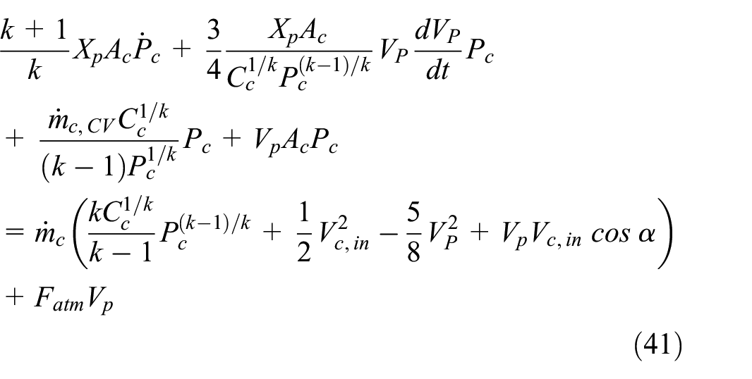
It is a first-order nonlinear ordinary differential equation for the pressure (P_c) inside the cylinder. The initial conditions for $P_c$ (e.g., $P_c\left(0\right)=A$ ) are obtained from the first stage of exhaust gas in the tank.

Modeling of mechanical system

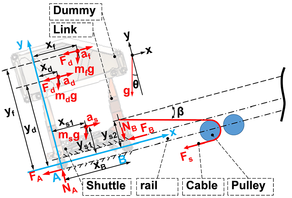
The mechanical system includes (a) a fixed rail, (b) a shuttle moving along the rail, (c) an assumed rigid cable connected to the shuttle and the piston, (d) a pulley used to change the direction of the piston force, and (e) the dummy M carried by the shuttle that includes the dummy frame and dummy mass. The shuttle, dummy frame, and dummy mass are shown in Figure 6.

Figure 6.

The component of the shuttle $m_s$ , dummy frame $m_f$ , and dummy mass $m_d$ .

In order to simplify the mathematical model, the following assumptions are made for the mechanical system: (10) compare with the masses of the shuttle and the dummy, the mass of the cable, the pulley, and the piston can be neglected; (11) The motion of the mechanical components is regarded as the rigid body plane motion; (12) Ignore the drag force on the dummy and shuttle during the launching process. (13) The dummy and the shuttle do not separate during launching before reaching the third stage.

The launching process of the dummy is divided into three stages. The first stage is the time duration when the shuttle is kept stationary at an original place; the second stage is the acceleration process of the shuttle and the dummy, and the third stage denotes the instant beyond which the dummy starts to separate from the shuttle. In this study, we focus primarily only on the launching system’s performance in achieving the highest speed during the first and second stages.

First stage

The free-body diagram of the first stage is shown in Figure 7 for the mechanical system. The pull force $F_s$ provided by the cable maintains a static equilibrium for the whole system. Based on assumption (10), the mass of the cable and the pulley are neglected. The lower rail exerts normal forces $N_A$ and $N_B\prime$ on the wheels A and B, respectively. These forces are in static equilibrium with the masses of the shuttle $m_s$ , the dummy mass $m_d$ , and the dummy frame $m_f$ . At this stage, the wheels have not yet generated frictional forces.

Figure 7.

The free-body diagram of the first stage. ⁷

According to Newton’s 2nd law, the force balance in the x direction is shown in equation (42).

$$F_s\cos \beta -(m_s+m_f+m_d)g\sin \theta =0$$

(42)

The total force applied to the shuttle in the y direction is zero and is shown as equation (43).

$$2N_A+2N{\prime }_B-(m_s+m_f+m_d)g\cos \theta -F_s\sin \beta =0$$

(43)

The sum of the moment about the wheel A of all the external forces is zero ( $\sum M_A=0$ ), as shown in equation (44).

$$\begin{array}{c}-2{N\prime }_B{x}_B+F_s\cos \beta y_{s2}+F_s\sin \beta x_B-m_{s}g\sin \theta y_{s1}\hfill \\ +m_{s}g\cos \theta x_{s1}-m_{f}g\sin \theta y_f+m_{f}g\cos \theta x_f\hfill \\ -m_{d}g\sin \theta y_d+m_{d}g\cos \theta x_d=0\hfill \end{array}$$

(44)

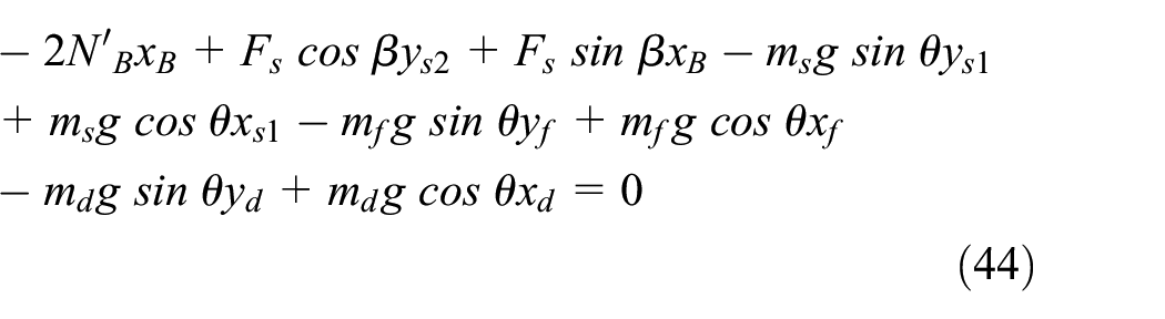
Solve equations (42)–(44), the results of $F_s$ , $N_B\prime$ , and $N_A$ are shown as equations. (45)–(47) in the first stage.

$$F_s=C_1/\cos \beta$$

(45)

$$N_B\prime =\frac{\cos \beta y_{s2}+\sin \beta x_B}{2x_B}{F}_s+\frac{C_4-C_3}{2x_B}$$

(46)

$$N_A=\frac{C_2+F_s\sin \beta }{2}-N_B\prime$$

(47)

Where $C_1$ , $C_2$ , $C_3$ , and $C_4$ are shown in equations (48)–(51).

$$C_1=(m_s+m_f+m_d)g\sin \theta$$

(48)

$$C_2=(m_s+m_f+m_d)g\cos \theta$$

(49)

$$C_3=(m_s{y}_{s1}+m_f{y}_f+m_d{y}_d)g\sin \theta$$

(50)

$$C_4=(m_s{x}_{s1}+m_f{x}_f+m_d{x}_d)g\cos \theta$$

(51)

Second stage

The second stage denotes the duration when the shuttle from a static state, including three steps depicted in Figure 8. (a) Shuttle overcomes the maximum static friction between the wheel and the rail; (b) Shuttle starts to accelerate and move forward; (c) The front wheels of the shuttle are lifted and accelerated continuously.

Figure 8.

The shuttle’s motion behavior during the three phases of the acceleration process: (a) Overcomes the maximum static friction; (b) Starts to accelerate and move forward; (c) The front wheels of the shuttle are lifted.

Overcoming maximum static friction

The shuttle will start to move forward until it overcomes the maximum static friction. The free-body diagram of the whole system during this stage is depicted in Figure 9. After the valve of the pneumatic tank opens, the pull force $F_s$ by the piston increases. However, at the initial moment, the displacement, velocity, and acceleration of the shuttle are still zero. Not until the pull force $F_s$ overcome the maximum static friction $F_A$ and $F_B\prime$ , the shuttle starts to move forward. Within this duration, the lower rail exerts normal forces $N_A$ and $N_B\prime$ on the wheels A and B, respectively. These forces balance the masses of the shuttle $m_s$ , the dummy mass $m_d$ , and the dummy frame $m_f$ .

Figure 9.

The free-body diagram when the shuttle overcomes the maximum static friction force. ⁷

According to Newton’s $2^{\mathrm{nd}}$ law, the force balance in the x direction is shown in equation (52).

$$F_s\cos \beta -(m_s+m_f+m_d)g\sin \theta -2F_A-2F{\prime }_B=0$$

(52)

The force balance in the y direction is zero and is shown as equation (53).

$$2N_A+2N{\prime }_B-(m_s+m_f+m_d)g\cos \theta -F_s\sin \beta =0$$

(53)

The sum of the moment of the external forces ( $F_s,F_A,F_B^{\prime },N_A,N_B^{\prime },m_{s}g,m_{d}g,m_{f}g$ ) about A is zero ( $\sum M_A=0$ ), as shown in equation (54).

$$\begin{array}{c}-2N{\prime }_B{x}_B+F_s\cos \beta y_{s2}+F_s\sin \beta x_B-m_{s}g\sin \theta y_{s1}\hfill \\ +m_{s}g\cos \theta x_{s1}-m_{f}g\sin \theta y_f+m_{f}g\cos \theta x_f\hfill \\ -m_{d}g\sin \theta y_d+m_{d}g\cos \theta x_d+(2F_A+2F{\prime }_B)r=0\hfill \end{array}$$

(54)

Solving the equations (52)—(54), the results of $F_s$ , $N_B\prime$ , $N_A$ , $F_A$ , and $F{\prime }_B$ are shown as equations (55)–(59). The result of $F_s$ can overcome maximum static friction $F_A$ and $F_B\prime$ .

$$F_s=\frac{C_1+{\mu }_s{C}_2}{\cos \beta +{\mu }_s\sin \beta }$$

(55)

$$\begin{array}{c}\multicolumn{1}{c}{N_B\prime =\frac{\cos \beta y_{s2}+\sin \beta x_B+\sin \beta {\mu }_{s}r}{2x_B}{F}_s}\\ +\frac{-C_3+C_4+{\mu }_{s}r{C}_2}{2x_B}\hfill \end{array}$$

(56)

$$N_A=\frac{C_2+F_s\sin \beta }{2}-N_B\prime$$

(57)

$$F_A={\mu }_s{N}_A$$

(58)

$$F_B\prime ={\mu }_s{N}_B\prime$$

(59)

Where the μ_s is the static friction coefficient between the wheels and the rail.

The shuttle start to move forward

Figure 10 illustrates the free-body diagram depicting the forces acting on the shuttle and the dummy, which have overcome the maximum static friction and starts accelerating forward. Based on assumptions (8), (10), and (11) the mass of the cable and pulley can be neglected, and the force $F_s$ from the piston can fully transfer to the shuttle via the cable, and the motion of the shuttle and the dummy only move on the x-y plane. Based on assumption (12), the drag force $F_d$ on the shuttle and dummy are neglected during the accelerating process. As the pneumatic cylinder pressure rises, the pull force $F_s$ increases. The shuttle begins to move forward with an acceleration, $a_s$ , and the dummy moves forward with an acceleration $a_d$ . Based on assumption (13), the shuttle and the dummy move together and have the same displacement, velocity, and acceleration. Within this duration, we will unify both accelerations as $a_d$ .

Figure 10.

The free-body diagram of the shuttle starts to move forward. ⁷

According to Newton’s $2^{\mathrm{nd}}$ law, the force balance in the x direction is shown in equation (60).

$$\begin{array}{c}{F}_s\cos \beta -(m_s+m_f+m_d)g\sin \theta -(2F_A+2F{\prime }_B)\hfill \\ =(m_s+m_f+m_d)a_d\hfill \end{array}$$

(60)

The total force applied to the shuttle during the movement in the y direction is zero and is shown as equation (61)

$$2N_A+2N_B\prime -(m_s+m_f+m_d)g\cos \theta -F_s\sin \beta =0$$

(61)

The sum of the moment ( $\sum M_A$ ) of all the external forces ( $F_s,F_A,F_B^{\prime },N_A,N_B^{\prime },m_{s}g,m_{d}g,m_{f}g$ ) equals the moment of $m_s{a}_s$ , $m_d{a}_d$ , and $m_f{a}_f$ about wheel A ( $\sum {\left[M_k\right]}_A$ , defined in the kinetic diagram of Hibbeler ⁹ ), and is shown in equation (62).

$$\begin{array}{c}{F}_s\cos \beta y_{s2}+F_s\sin \beta x_B+(2F_A+2F{\prime }_B)r-2N{\prime }_B{x}_B\hfill \\ +(m_s{x}_{s1}+m_f{x}_f+m_d{x}_d)g\cos \theta \hfill \\ -(m_s{y}_{s1}+m_f{y}_f+m_d{y}_d)g\sin \theta \hfill \\ =(m_s{y}_{s1}+m_f{y}_f+m_d{y}_d)a_d\hfill \end{array}$$

(62)

Solving equations (60)–(62), the results of $a_d$ , $N_B\prime$ , $N_A$ , $F_B\prime$ , and $F_A$ are shown as equations (63)–(67).

$$a_d=\frac{\cos \beta -{\mu }_d\sin \beta }{C_5}{F}_s-C_6$$

(63)

$$\begin{array}{c}{N}_B\prime =\hfill \\ [\frac{\cos \beta y_{s2}+\sin \beta x_B+\sin \beta {\mu }_{d}r}{2x_B}-\frac{(\cos \beta -{\mu }_d\sin \beta )C_7}{2x_B{C}_5}]F_s+C_8\hfill \end{array}$$

(64)

$$N_A=\frac{C_2+F_s\sin \beta }{2}-N_B\prime$$

(65)

$$F_B\prime ={\mu }_d{N}_B\prime$$

(66)

$$F_A={\mu }_d{N}_A$$

(67)

Where the μ_d is the coefficient of kinetic friction between the wheels and the rail. $C_5$ , $C_6$ , $C_7$ , and $C_8$ are shown in equations (68)–(71).

$$C_5=(m_s+m_f+m_d)$$

(68)

$$C_6=\frac{C_1+{\mu }_d{C}_2}{C_5}$$

(69)

$$C_7=(m_s{y}_{s1}+m_f{y}_f+m_d{y}_d)$$

(70)

$$C_8=\frac{C_4-C_3+{\mu }_{d}r{C}_2+C_6{C}_7}{2x_B}$$

(71)

The front wheels of the shuttle are lifted

While the pull force $F_s$ is applied to the shuttle, the shuttle pivots around wheel A, and thus the front wheel B will be lifted. Consequently, the normal force on the front wheel B is now exerted by the upper rail in the -y direction as $N_B$ to maintain the shuttle’s forward motion without rotation, and the frictional force is in the -x direction as $F_B$ . Before the dummy separates from the shuttle, the dummy, and the shuttle are considered as a single body with the velocity $V_d$ and the acceleration $a_d$ . The free-body diagram depicted the forces acting on the shuttle and the dummy is shown in Figure 11.

Figure 11.

The free-body diagram of the shuttle and dummy when the front wheels of the shuttle are lifted. ⁷

According to Newton’s $2^{\mathrm{nd}}$ law, the force balance in the x direction is shown in equation (72).

$$\begin{array}{c}{F}_s\cos \beta -(m_s+m_f+m_d)g\sin \theta -2F_A-2F_B\hfill \\ =(m_s+m_f+m_d)a_d\hfill \end{array}$$

(72)

The total force in the y direction is zero and is shown as equation (73).

$$2N_A-2N_B-(m_s+m_f+m_d)g\cos \theta -F_s\sin \beta =0$$

(73)

When the shuttle moves forward, the sum of the moments ( $\sum M_A$ ) of the external forces ( $F_s$ , $F_A$ , $F_B$ , $N_A$ , $N_B$ , $m_{s}g$ , $m_{d}g$ , $m_{f}g$ ) equals the moments of $m_s{a}_s$ , $m_d{a}_d$ , and $m_f{a}_f$ about wheel A ( $\sum {\left[M_k\right]}_A$ , defined in the kinetic diagram ⁹ ), and is shown in equation (74).

$$\begin{array}{c}{F}_s\cos \beta y_{s2}+F_s\sin \beta x_B+(2F_A-2F_B)r+2N_B{x}_B\hfill \\ +(m_s{x}_{s1}+m_f{x}_f+m_d{x}_d)g\cos \theta \hfill \\ -(m_s{y}_{s1}+m_f{y}_f+m_d{y}_d)g\sin \theta \hfill \\ =(m_s{y}_{s1}+m_f{y}_f+m_d{y}_d)a_d\hfill \end{array}$$

(74)

Solving equations (72)–(74), the results of $a_d$ , $N_B$ , $N_A$ , $F_B$ , and $F_A$ are shown in equations (75)–(79).

$$\begin{array}{c}{a}_d=\hfill \\ (\frac{\cos \beta y_{s2}+\sin \beta x_B+{\mu }_{d}r\sin \beta }{(C_7+2x_B{C}_{10})}+\frac{2x_B\cos \beta -2x_B{\mu }_d\sin \beta }{4{\mu }_d(C_7+2x_B{C}_{10})})\hfill \\ F_s+C_{11}\hfill \end{array}$$

(75)

$$N_B=\frac{\cos \beta -{\mu }_d\sin \beta }{4{\mu }_d}{F}_s-C_9-C_{10}{a}_d$$

(76)

$$N_A=N_B+\frac{C_2+F_s\sin \beta }{2}$$

(77)

$$F_B={\mu }_d{N}_B$$

(78)

$$F_A={\mu }_d{N}_A$$

(79)

Where $C_9$ , $C_{10}$ , and $C_{11}$ are shown in equations (80)–(82).

$$C_9=\frac{C_1+{\mu }_d{C}_2}{4{\mu }_d}$$

(80)

$$C_{10}=\frac{C_5}{4{\mu }_d}$$

(81)

$$C_{11}=\frac{{\mu }_{d}r{C}_2-2x_B{C}_9+C_4-C_3}{(C_7+2x_B{C}_{10})}$$

(82)

Solve the pneumatic and mechanical system

Based on assumption (8) and (10), the pull force $F_s$ acting on the shuttle can be calculated using equation (25). The displacement $D_d$ and velocity $V_d$ of the shuttle is the same as $X_p$ and $V_p$ on cylinder piston.

The dummy velocity $V_d$ , shuttle velocity $V_s$ , and piston velocity $V_p$ can be obtained by integrating the acceleration of the shuttle, $a_d$ . The dummy displacement $D_d$ , shuttle displacement $D_s$ , and piston displacement $X_p$ can then be obtained by integrating the velocity of the shuttle $V_p$ , as shown in equations (83) and (84).

$$V_s\left(t\right)=V_d\left(t\right)=V_P(t)=\underset{0}{\overset{t}{\int }}{a}_d(t)\mathrm{dt}$$

(83)

$$D_d(t)=X_P(t)=\underset{0}{\overset{t}{\int }}{V}_P(t)\mathrm{dt}$$

(84)

In this study, equations (17), (25), and (41) in pneumatic system and equations (55), (58), (59), (63), (66), (67), (75), (78), (79), (83), and (84) in mechanical system will be solved simultaneously to find the solutions of $P_t(t)$ , $P_c(t)$ , $F_s\left(t\right)$ , $F_A\left(t\right)$ , $F_B\left(t\right)$ , $a_d\left(t\right)$ , $V_d\left(t\right)$ , and $D_d(t)$ . In this study, the above counpled nonlinear differential equations will be solved using the fourth-order Runge-Kutta method because of the numerical accuracy and stability by specifying the initial condition of $P_{t,0}$ and $P_{c,0}$ .

In this study, the PL-40 launching system is used as the research target, with a dummy ( $\mathrm{M}=m_f+m_d$ ) replacing the UAV to establish a mathematical model. The masses and coordinates of the shuttle and dummy are listed in Table 1. This study will refer to the conditions in Lee et al. ⁷ ’s study to investigate the launching conditions of UAVs with different masses. By changing the value of, the performance of the launching system under varying UAV masses can be analyzed. The parameters required for the mathematical model analysis of the launching system, including those for the pneumatic and mechanical systems, are shown in Table 2. If it is necessary to adjust the design parameters of the launching system to study the effect of different launching system sizes on UAV launch velocity, this can be achieved by modifying the parameters in Tables 1 and 2.

Table 1.

The coordinate of the shuttle, dummy frame, and dummy mass.

Name	Mass (kg)	x (mm)	y(mm)	z (mm)
$m_s$	1.32	$x_{s1}$ (125)	$y_{s1}$ (50)	0
Wheel A	N.A.	0	0	0
Wheel B	N.A.	$x_B$ (200)	0	0
$F_s$	N.A.	$x_B$ (200)	$y_{s2}$ (60)	0
$m_f$	10	$x_f$ (68)	$y_f$ (264)	0
$m_d$	0/10/20	$x_d$ (78)	$y_d$ (278)	0

Table 2.

The parameter in pneumatic and mechanical systems.

Pneumatic system		Mechanical system
parameter	value	parameter	value
B	0.528	Ld	3128 mm
Dp	50 mm	$m_s$	1.32 kg
k	1.4	$m_f$	10 kg
Pa	1 atm	$m_d$	0/10/20 kg
Pt_g	10 bar	r	15 mm
R	287.1	θ	11°
S	367 mm2	μd	0.12
${\forall }_{\mathrm{t}}$	24 L	μs	0.15

Results and discussions

Comparison of predicted velocity with experimental results

The same launching conditions ( $m_f=10\mathrm{kg}$ , $m_d=0\mathrm{kg}$ , and $P_{t\_g}=10\mathrm{bar}$ ) as Lee et al. ⁷ ( $\mathrm{M}=m_f+m_f=10\mathrm{kg},\mathrm{and}{P}_{t\_g}=10\mathrm{bar})$ were used to verify the correctness and accuracy of the proposed multi-physical model in this study.

The time variation of the predicted tank pressure in Figure 12(a) follows a trend consistent with the experimental results. Comparison of the air cylinder pressures of the predicted results with those of the experimental ones in Figure 12(b), the trends of both cylinder pressures over the studied time duration are consistent. However, the predicted cylinder pressure is significantly higher than that of the experimental results beyond the instant t = 0.15 s (or t > 0.15 s). This study derives that the pressure change of the air pressure system during the launch process is assumed to have no influence from head loss and minor loss. Because the influence of head loss and minor loss is not considered, it can be seen from Figure 12(a) and (b) that the pressure $P_{t\_g}$ of the tank and he pressure $P_{c\_g}$ of the cylinder overlap in the numerical analysis result. Comparing the pressure of the cylinder in Figure 12(b) with the experimentally measured pressure value, it can be found that the cylinder pressure $P_{c\_g}$ obtained through mathematical model is higher than the experimental result.

Figure 12.

Comparison between multi-physical results and various experiments in time-variations during the launching process (a) Tank pressure, (b) Cylinder pressure, (c) Dummy acceleration, (d) Dummy displacement. (e) Dummy velocity. ( $m_f=10\mathrm{kg}$ , $m_d=0\mathrm{kg}$ , $P_{t\_g}$  = 10 bar).

As is shown in equation (25), the pull force $F_s$ is proportional to $P_c$ , the predicted results of the pull force should be noticeably higher than those of the experimental results within the same time duration. Further, the time variation in the pull force can be related to the time variation in shuttle acceleration shown in Figure 12(c), where the predicted shuttle acceleration is higher than those of the experimental results beyond the instant t = 0.15 s. The dummy velocity acquired by the proposed multi-physical model was compared with the experimental results. Figure 12(d) shows that the variation of the dummy velocity over time is consistent with the experimental results. As the same trend in Figure 12(b) and (c), the predicted velocity of the dummy in Figure 12(d) is significantly higher than that of the experimental results beyond the instant t = 0.15 s (or t > 0.15 s). This higher predicted result is caused by the assumption of no head loss in the proposed model. If the head losses in the tank and the cylinder are considered, this discrepancy can be reduced. The maximum velocity of the dummy in the experimental results is 24.4 m/s, while the calculated velocity in this study is 26.6 m/s, resulting in a 9.0% relative error, calculated as $|V_d-V_d^{*}|/|V_d{|}^{10}$ . Here, $V_d\ne 0$ and $V_d^{*}$ is an approximation of $V_d$ . In this study, represents the result from the mathematical model, while $V_d$ corresponds to the experimental result. Finally, the time variation of the predicted shuttle displacement over the time duration is depicted in Figure 12(e), which also shows the same trend as those of the experimental results.

The comparisons of the mathematical predicted results with the experimental results are shown in Figure 12. It can be observed that when $m_f=10\mathrm{kg}$ , $m_d=0\mathrm{kg}$ , and $P_{t\_g}=10\mathrm{bar}$ , the trends in the mathematical predicted results for $P_{t\_g}$ , $P_{c\_g}$ , $a_d$ , $V_d$ , and $D_d$ align with the experimental trends reported in Lee et al. ⁷ ’s study. In order to validate that the mathematical model is suitable for different conditions, the condition of is changed from 0 to 10 and 20 kg. Namely, that M is equal to 20 and 30 kg in Lee et al. ⁷ ’s study. The results of P _t _ _g , P _c _ _g , and v and were compared with Lee’s experiments. Figure 13(a) and (b) show the comparison results of $P_{t\_g}$ , $P_{c\_g}$ , and $V_d$ between the mathematical model and the experimental results. While compare the trend of the curve $P_{c\_g}$ , and $V_d$ in Figure 12, the $P_{c\_g}$ is also higher than the experiment result so that the $V_d$ is also higher than the experiment result. This consistency demonstrates that the mathematical model provides reliable predicted results under various conditions. The maximum velocities of $V_d$ from the mathematical model and the experimental results are shown in Table 3, where the maximum error of $V_d$ is 9.0. Based on previous assumptions (4), (8), and (10), this study assumes that head loss has no impact, the cable is rigid, and the masses of both the cable and pulley are negligible. The actual launching system in this research aligns with these assumptions, resulting in the calculated displacement, maximum velocity, and acceleration of the dummy in the multi-physics mathematical model being very close to the experimental results. However, if the design of the launching system cannot meet these assumptions due to specific requirements, it may affect the study’s findings.

Figure 13.

Comparison between multi-physical results and various experiments in different dummy masses (a) $m_f=10\mathrm{kg}$ , $m_d=10\mathrm{kg}$ , $P_{t\_g}$  = 10 bar (b) $m_f=10\mathrm{kg}$ , $m_d=20\mathrm{kg}$ , $P_{t\_g}$  = 10 bar.

Table 3.

The comparison of experiment and mathematical results.

			Mathematical result (m/s)	Experiment 7 (m/s )
$P_{t\_g}$ (bar)	$m_f$ (kg)	$m_d$ (kg)	$V_d$ (m/s)	$V_d$ (m/s)
				#1	#2	#3	#4	#5	#6	$\overline{X}$	Error(%)
10	10	0	26.6	24.4	24.3	24.4	24.3	24.6	24.3	24.4	9.0
10	10	10	19.2	18.4						N.A.	4.3
10	10	20	15.7	14.4						N.A.	9.0

The frictional force of multi-physics numerical result

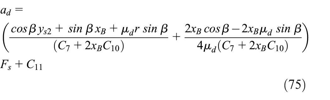
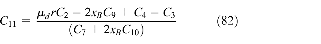
The explanation provided in the preceding section confirms the correctness and reliability of the multi-physical model. The mathematical models of the shuttle are derived in this paper, the frictional force and acceleration of the shuttle are described in equations (75), (78), and (79). As shown in Figure 14(a), both the friction force between the shuttle and the rail, as well as the shuttle’s acceleration, have a linear relationship with the pull force in the shuttle. It can be found that the trend of the frictional force and acceleration related to the pull force of the shuttle of the mathematical models are consistent with Lee et al. ⁷ ’s co-simulation results. That is, the frictional force in the acceleration process is related to the pull force.

Figure 14.

(a) Pull force-variations of acceleration for the dummy and the frictional force between the shuttle and rail. (b) The frictional forces on shuttle wheels ( $m_f=10\mathrm{kg}$ , $m_d=0\mathrm{kg}$ , $P_{t\_g}$  = 10 bar).

Equations (78) and (79) determine $F_B$ and $F_A$ , representing the frictional forces on one side of the front and rear wheels of the shuttle, respectively. While launching the dummy, the actual frictional force between the shuttle and the rail is the sum of the frictional forces of all four shuttle wheels ( $F_{\mathrm{total}}=2F_A+2F_B$ ). The variation in friction between the shuttle and the rail during the acceleration process is shown in Figure 14(b). As the cylinder pressure decreases during acceleration, the frictional force gradually declines. A comparison with the frictional force obtained through the co-simulation analysis by Lee et al. ⁷ shows that the trend of frictional force variation is consistent.

In the studies by Francis, ² Novaković and Medar, ³ and Siddiqui et al., ⁶ only the frictional force generated by the dummy’s gravity is considered, as indicated by F_Ref in Figure 14(b). In this study, the maximum frictional force during the acceleration process is 316N, whereas the frictional force considering only the dummy’s gravity, based on the studies by Francis, ² Novaković and Medar, ³ and Siddiqui et al. ⁶ is 13N. The frictional force generated by the pull force of the shuttle is much greater than that produced by the gravity of the dummy and the shuttle.

Conclusions

This study is the first to apply a multi-physical method combining mechanical and pneumatic mathematical models to solve engineering problems related to launching systems. This study first applies the multi-physical mathematical model to predict the performance of the launching system, including the displacement, velocity, and acceleration of the dummy, as well as the pressure of the tank and cylinder. This approach can achieve results close to those obtained through the realistic experiments. ⁷ The parameters of the multi-physics mathematical model can be adjusted according to the actual conditions, offering great design flexibility and potentially significant cost savings compared with that of expensive analyzing software.

The multi-physical model is utilized in this study to estimate the velocity of the launching dummy. The trend of the dummy’s velocity over time matched the experimental results, with a maximum error of 9.0% and a minimum error of 4.3%. The trends of the curves for tank pressure, cylinder pressure, shuttle displacement, and acceleration over time also closely corresponded with the experimental results.

Furthermore, this study revealed a linear relationship between the frictional and pull forces, consistent with findings from Lee et al. ⁷ The friction force generated by the pull force was significantly greater than that produced by the shuttle and dummy gravity, aligning with the results of Lee et al. ⁷

Currently, this study does not account for head loss and minor losses, which may lead to higher pressure values in the pneumatic cylinder within the multi-physical model, resulting in greater acceleration and velocity of the dummy. The masses of the cable and pulley may also influence the results. Future research works will incorporate head loss and minor losses in the tank and cylinder, as well as the masses of the cable and pulley, to more accurately estimate the performance of the launching system.