Predictive residual stress analysis in gear units: an artificial intelligence approach based on finite element data

Abstract

Determining residual stresses is essential for ensuring the safety and longevity of gear components. Traditional methods, such as analytical, numerical, and experimental approaches, are often costly, time-consuming, and sometimes destructive. This study proposes a new method to predict residual stresses in gear units using artificial intelligence based on data from finite element analysis. To achieve this, a commercial finite element tool models the heat treatment and carburization processes, grounded in thermomechanical metallurgical physics. The residual stresses obtained from finite element analysis are then compared to the ones from experiment using deep hole drilling approach. This is followed by a sensitivity analysis. Next, a specific class of gearbox component geometries and the computed stress fields are utilized to train artificial neural networks. The performance of the artificial neural networks approach is compared to that of two different machine learning regression methods. It has been concluded that this technique successfully anticipates residual stresses in components with scaled geometries and similar heat treatment steps, outperforming the two regression models in accuracy and efficiency. Importantly, it achieves this with incomparable, significantly less computation time compared to standard finite element analysis.

Introduction

In turbo gear units ¹ with up to 100,000 rpm, residual stresses can significantly impact the component’s lifespan, potentially leading to premature failure. These stresses arise mainly from thermal shrinkage/expansion coupled with phase transformations especially during the quenching step of heat treatment processes and can reach critically high levels similar to those induced by centrifugal forces. Investigating and understanding the distribution of the residual stresses has thus become an inseparable part of the fracture mechanics analysis of a gearwheel. To this end, various experiments, as in the review work of Schajer and Ruud ² as well as numerical methods have evolved over the last few decades.

Experimental methods to determine residual stresses are divided mainly into (semi) destructive and nondestructive approaches. ² Nondestructive methods such as X-ray diffraction, ultrasonic, and magnetic methods measure some material parameters which are related to stresses while most of destructive method are carried out by material removal. As a result, deformations due to the release of stresses are measured. Hole drilling, sectioning, slotting, and deep hole drilling belong to this category. For a detailed comparison of these methods, refer to Rossini et al. ³ Additionally, Serasli et al. ⁴ conducted a study on the technical challenges of certain destructive methods compared to the neutron diffraction method. Taraphdar et al. ⁵ and Jhunjhunwala et al. ⁶ provided examples of deep hole drilling experiments for determining weld-induced residual stresses. They measured through-thickness stresses and compared these with predictions from 2D and 3D finite element simulations. As a downside, most experimental methods for determining stresses within the material core tend to be prohibitively expensive or destructive.

In response to this challenge, numerical methods have emerged as reliable alternatives, circumventing the need for destructive tests. The physics of quenching and carburizing was modeled by Shao et al. ⁷ to anticipate and reduce the distortion in a steel gear due to heat treatment. Analogously, Esfahani ⁸ investigated the microstructure and stress distribution on martensitic transformation of steel gears during heat treatments. Waimann and Reese ⁹ developed a thermomechanically coupled variational material model to simulate phase transformations among austenite, ferrite, and martensite induced by thermal processes. Bammann et al. ¹⁰ developed a commercial tool to simulate carburizing as well as quenching for steels experiencing phase transformations. He et al. ¹¹ examined the impact of initial residual stresses on the fatigue failure analysis of gears within the framework of continuum damage mechanics. Nevertheless, due to the intricate metallurgical thermomechanical physics involved, simulations can become arduous and time-consuming.

To alleviate this issue, different machine learning regression models have emerged as an alternative to conventional FE analysis. Although these methods require several FE simulations for their input, they can be advantageous for repetitive prediction of a model behavior. Liang et al. ¹² used a deep learning (DL) model to anticipate the stresses in aortic wall of a human being to avoid time-consuming clinical applications. The mechanical response of elasto-viscoplastic grain microstructures were modeled applying artificial neural network by Khorrami et al. ¹³ Their method showed to be 500 times faster than the numerical solution of the initial boundary value problem. Concli et al. ¹⁴ employed a hierarchical structure of artificial neural networks (ANNs) for detection of pitting damage positioned on the teeth flank, significantly enhancing prediction accuracy. Schoop et al. ¹⁵ developed a physics-informed, data-driven semi-analytical model to predict residual stresses. This approach significantly reduced the need for extensive experimental testing and complex finite element (FE) simulations. Further details regarding the physics-informed neural networks (PINNs) can be found in the work of Rezaei et al. ¹⁶ and Harandi et al. ¹⁷

For the structural and fracture analysis of gears, it is crucial to efficiently determine residual stresses arising from manufacturing thermal processes in terms of both cost and time. Computing these stresses individually using commercial finite element (FE) tools can take over a day, which is often impractical for real-world industrial applications. To address this challenge, this paper introduces a novel artificial neural network (ANN) model that reduces the computation time to mere seconds. To the best of the authors’ knowledge, no similar machine learning method has been proposed for this purpose. This study is the first to explore the mapping of 2D stress fields across various gear geometries of the same material, subjected to comparable heat treatments. The proposed method produces highly reliable stress fields when compared to both FE simulations and experimental results.

The structure of this paper is as follows. First, the theory behind the thermomechanical metallurgical physics of the problem based on the work of Bammann et al. ¹⁰ is introduced briefly. Then, a commercial finite element tool is utilized to simulate heat treatment process and subsequently assess residual stresses in diverse gearbox components. The simulation results are compared to experimental values obtained from the (incremental) deep hole drilling method. Sensitivity analyses are conducted to study the influencing factors on the formation of the residual stresses. Next, the study categorizes several two-dimensional stress fields for scaled geometries of reference geometry. These stress values are used in three different machine learning models: artificial neural networks (ANNs), random forest regression (RFR), and support vector regression (SVR). The artificial neural networks (ANNs) outperform the other regression approaches. Ultimately, the predicted stress values are validated with the FE and the test results. In this way, stress values at an arbitrary position for a class of geometries is obtained.

Materials and methods

Governing equations

Modeling the metallurgical aspects of heat treatment coupled to the thermomechanical physics of the problem is briefly addressed here based on the work of Bammann et al. ¹⁰ The exact model used by the commercial user material subroutine DANTE ¹⁸ is not accessible due to confidentiality.

Heat treatment of the material involves the heating up of the part in the furnace and keeping it at a high temperature while being carburized. Next, the part is oil quenched, and the temperature drops suddenly. After a transfer time, the component goes through two tempering cycles to relieve a level of residual stresses, refer to Figure 4. For confidentiality reasons, x and y-axes are normalized with respect to the quench time, carburizing temperature, and the base carbon potential, respectively.

Due to the microstructural aspects of the heat treatment and quenching in austenitic low carbon steels, additional phase transformations induced macroscopic plasticity is considered besides the thermal and mechanical aspects. This can significantly influence the residual stresses and distortions ¹⁰

The adopted modeling approach integrates differential equations for phase evolution with a multiphase macroscopic state variable material model. ¹⁰ Kinetic rate equations for each product phase are established using a thermodynamic framework, aligned with experimental data. Unlike traditional models, Bammann et al. ¹⁰ employ mixture theory to track individual phase behavior, incorporating internal stresses to model phase interactions and capturing both macroscopic multiphase behavior and transformation-induced effects.

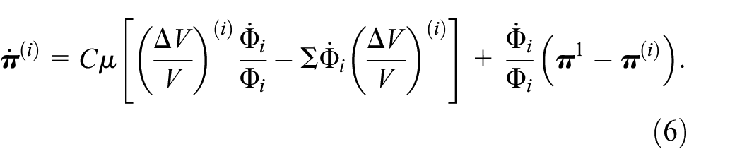
The strain rate for transformation plasticity is given by ¹⁹ :

$${\stackrel{·}{\mathit{\epsilon }}}^{\mathrm{TR}}=\frac{K}{{\mathrm{\Sigma }}_y}\left(\frac{\mathrm{\Delta }V}{V}\right)\mathbf{\Psi }\left(\mathrm{\Phi }\right)\stackrel{·}{\mathrm{\Phi }}\mathit{\sigma ́},$$

(1)

where $\mathit{\sigma ́}$ is the stress deviator, $\stackrel{·}{\mathrm{\Phi }}$ represents the rate of the change of the volume fraction, $\mathrm{\Delta }V/V$ is the volume misfit and ${\mathrm{\Sigma }}_y$ denotes the yield strength of the weaker phase. Due to the proportionality of the transformation plastic strain rate in equation (1) on the deviatoric stress and not on its rate, the additional plasticity can be represented using a formulation based on a state variable.

The internal state variable model is based on the kinematics of the large deformation elastoplasticity. Here, the free energy and the stress are dependent on elastic strain, temperature, strain rate, and the current values of internal variables introduced to characterize the material state. These state variables are linked to fundamental micro-mechanisms that are presumed to govern the macroscopic response across various temperatures and strain rates. On the macroscopic scale, incorporating these variables leads to the predicting of material response dependent on the history of strain rate and temperature.

Bammann ¹⁰ introduced a tensor variable $\mathbf{\alpha }$ , (backstress or kinematic hardening variable) and a scalar variable $\kappa$ , (isotropic hardening variable) along with corresponding evolution equations. The evolution of these state variables follows a standard hardening minus recovery format, incorporating both dynamic and thermal recovery terms.

In multiphase materials, predicting response is complicated by phase transformation-induced plastic strain. Cooling steel triggers solid-state transformations, yielding product phases with larger volume and greater hardness than austenite. This results in a forward stress ${\mathit{\pi }}^{(i)}$ in austenite ( $i=1$ ), causing apparent softening. Additionally, backward stresses, ${\mathit{\pi }}^{(i)}$ arise in product phases ( $i=2-5$ : pearlite, ferrite, bainite, martensite).

In a generalized state variable model for multiphase materials, each point in the continuum can host all phases simultaneously. Each phase follows a single-phase state variable model with rate and temperature dependence. The deviatoric Cauchy stress in each phase is denoted as $\mathit{\sigma ́}(i)$ , and a classic volume fraction-weighted rule of mixtures determines the total deviatoric Cauchy stress $\mathit{\sigma ́}$

$$\mathit{\sigma ́}=\sum _i{\mathrm{\Phi }}_i{\mathit{\sigma ́}}^{(i)};\sum _i{\mathrm{\Phi }}_i=1.$$

(2)

The symbol ${\mathrm{\Phi }}_i$ denotes the volume fraction for each phase, with the constraint that the sum of these phase volume fractions must equate to one. We employ a hypoelastic relation for each phase, consistent with the assumption of linear elasticity, resulting in

$$\mathit{\sigma ́}°=2\mu {\mathit{D́}}_e^{(i)}+\frac{\stackrel{·}{\mu }}{\mu }{\mathit{\sigma ́}}^{(i)}.$$

(3)

Here, ${\mathit{D́}}_e^{(i)}$ is the elastic symmetric component of the deviatoric velocity gradient, and $\mu$ is the shear modulus, which varies with temperature and is presumed uniform across all phases. We disregard the impact of the term associated with the time rate of change of the shear modulus. ${\mathit{D́}}_e^{(i)}$ is the elastic deformation rate, ¹⁰ given by

$${\mathit{D́}}_e^{(i)}=\mathit{D́}-{\mathit{D́}}_p^{\left(i\right)}-{\mathit{D́}}_{\mathrm{th}}^{(i)},$$

(4)

where $\mathit{D́}$ , ${\mathit{D́}}_p^{\left(i\right)}$ , ${\mathit{D́}}_{\mathrm{th}}^{(i)}$ are the total, inelastic, and sum of the thermal deformation rates, respectively. The notation in equation (3) represents the convective derivative of the Cauchy stress ¹⁰ as in

$$\mathit{\sigma ́}°(i)={\stackrel{·}{\mathit{\sigma }}}^{(i)}-{\mathit{W}}_e^{\left(i\right)}{\mathit{\sigma }}^{\mathbf{\left(}\mathbf{i}\mathbf{\right)}}+{\mathit{\sigma }}^{\mathbf{(}\mathbf{i}\mathbf{)}}{\mathit{W}}_e^{(i)},$$

(5)

with ${\mathit{W}}_e^{(i)}=\mathit{W}-{\mathit{W}}_p^{(i)}$ representing the skew part of the elastic velocity gradient for each respective phase. In this work, the Jaumann derivative is considered with all ${\mathit{W}}_p^{(i)}=0.$

Through an approximation of the compatibility between the hard and soft regions within the multiphase alloy, a self-consistent methodology ²⁰ was employed to derive an evolution equation for long range internal stresses that aligns with mixture theory

$${\stackrel{·}{\mathit{\pi }}}^{(i)}=C\mu [{\left(\frac{\mathrm{\Delta }V}{V}\right)}^{(i)}\frac{{\stackrel{·}{\mathrm{\Phi }}}_i}{{\mathrm{\Phi }}_i}-\mathrm{\Sigma }{\stackrel{·}{\mathrm{\Phi }}}_i{\left(\frac{\mathrm{\Delta }V}{V}\right)}^{(i)}]+\frac{{\stackrel{·}{\mathrm{\Phi }}}_i}{{\mathrm{\Phi }}_i}({\mathit{\pi }}^1-{\mathit{\pi }}^{\mathbf{\left(}\mathbf{i}\mathbf{\right)}}).$$

(6)

Next, we assume two short-range internal stress fields, ${\mathbf{\alpha }}^{\mathbf{\left(}\mathbf{i}\mathbf{\right)}}$ and ${\mathbf{\kappa }}^{\mathbf{\left(}\mathbf{i}\mathbf{\right)}}$ , operating locally within each phase. The net stress ¹⁰ in each phase is then defined as

$${\mathbf{\xi }}^{\mathbf{(}\mathbf{i}\mathbf{)}}={\mathit{\sigma ́}}^{(i)}-{\mathbf{\alpha }}^{\mathbf{\left(}\mathbf{i}\mathbf{\right)}}-{\mathbf{\kappa }}^{\mathbf{\left(}\mathbf{i}\mathbf{\right)}}-{\mathit{\pi }}^{\mathbf{\left(}\mathbf{i}\mathbf{\right)}}.$$

(7)

Assuming that ${\mathit{\pi }}^{\mathbf{\left(}\mathbf{i}\mathbf{\right)}}$ as ${\mathbf{\kappa }}^{\mathbf{\left(}\mathbf{i}\mathbf{\right)}}$ well as act in the direction of the Cauchy stress, we receive in each phase,

$${\mathit{\pi }}^{\mathbf{\left(}\mathbf{i}\mathbf{\right)}}={\mathit{\pi }}^{\left(i\right)}\frac{{\mathit{\sigma ́}}^{(i)}-{\mathbf{\alpha }}^{\mathbf{\left(}\mathbf{i}\mathbf{\right)}}}{|{\mathit{\sigma ́}}^{(i)}-{\mathbf{\alpha }}^{\mathbf{\left(}\mathbf{i}\mathbf{\right)}}|},{\mathbf{\kappa }}^{\mathbf{\left(}\mathbf{i}\mathbf{\right)}}={\kappa }^{\left(i\right)}\frac{{\mathit{\sigma ́}}^{(i)}-{\mathbf{\alpha }}^{\mathbf{\left(}\mathbf{i}\mathbf{\right)}}}{|{\mathit{\sigma ́}}^{(i)}-{\mathbf{\alpha }}^{\mathbf{\left(}\mathbf{i}\mathbf{\right)}}|}.$$

(8)

In this way, the effective stress resulting in plastic flow ¹⁰ is given by

$$|{\mathbf{\xi }}^{\mathbf{(}\mathbf{i}\mathbf{)}}|=|{\mathit{\sigma ́}}^{\left(i\right)}-{\mathbf{\alpha }}^{\mathbf{\left(}\mathbf{i}\mathbf{\right)}}|-{\kappa }^{\left(i\right)}-{\mathit{\pi }}^{\left(i\right)}$$

(9)

The plastic flow rule ¹⁰ is selected to exhibit a pronounced nonlinear dependence on the deviatoric stress,

$${\mathit{D}}_p^{\left(i\right)}=f^{\left(i\right)}\left(\theta \right)\sinh \left\{\frac{|{\xi }^{\left(i\right)}|-Y^{\left(i\right)}\left(\theta \right)}{V^{\left(i\right)}\left(\theta \right)(1+N\left(C\right))}\right\}\frac{{\mathit{\sigma ́}}^{(i)}-{\mathbf{\alpha }}^{\mathbf{\left(}\mathbf{i}\mathbf{\right)}}}{|{\mathit{\sigma ́}}^{(i)}-{\mathbf{\alpha }}^{\mathbf{\left(}\mathbf{i}\mathbf{\right)}}|}.$$

(10)

Here, $f^{\left(i\right)}\left(\theta \right)$ and $V^{\left(i\right)}\left(\theta \right)$ represent the rate dependence of the yield stress at a constant temperature, and $N(C)$ accounts for the yield increase with rising carbon content, $C$ . Tensor variables ${\mathbf{\alpha }}^{\mathbf{\left(}\mathbf{i}\mathbf{\right)}}$ and scalar variables ${\mathbf{\kappa }}^{\mathbf{\left(}\mathbf{i}\mathbf{\right)}}$ are introduced to depict the deformed state of each phase, as detailed earlier for a single-phase material. ²¹ The evolution of these variables ¹⁰ is defined separately for each phase.

$$\begin{array}{c}{\stackrel{·}{\kappa }}^{\left(i\right)}=H^{\left(i\right)}(\theta ,C)\left|{\mathit{D}}_p^{\left(i\right)}\right|-\{R_S^{\left(i\right)}\left(\theta \right)+R_D^{\left(i\right)}\left(\theta \right)\left|{\mathit{D}}_p^{\left(i\right)}\right|\}\left|{\kappa }^{\left(i\right)}\right|{\kappa }^{\left(i\right)},\\ {\stackrel{·}{\mathbf{\alpha }}}^{\left(i\right)}=h^{\left(i\right)}(\theta ,C){\mathit{D}}_p^{\left(i\right)}-\{r_S^{\left(i\right)}\left(\theta \right)+r_D^{\left(i\right)}\left(\theta \right)\left|{\mathit{D}}_p^{\left(i\right)}\right|\}\left|{\mathbf{\alpha }}^{\mathbf{\left(}\mathbf{i}\mathbf{\right)}}\right|{\mathbf{\alpha }}^{\mathbf{\left(}\mathbf{i}\mathbf{\right)}},\end{array}$$

(11)

where $R_D^{\left(i\right)}\left(\mathrm{\theta }\right)$ , $r_d^{\left(i\right)}\left(\mathrm{\theta }\right)$ and $R_s^{\left(i\right)}\left(\mathrm{\theta }\right)$ , $r_s^{\left(i\right)}\left(\mathrm{\theta }\right)$ are the temperature dependent isotropic/kinematic dynamic and static recovery content as a function of material parameters, respectively. The functions $H^{\left(i\right)}(\theta ,C)$ and $h^{\left(i\right)}(\theta ,C)$ are calculated from instantaneous temperature, carbon content and material parameters. ¹⁰

Multiphase transformation kinetics

A balance principle is employed to yield differential equations for the modeling of the phase transformation kinetics at a volume fraction. This naturally couples with the differential equations governing the mechanical and thermal aspects of a given process.^22,23 For clarity, we replace numerical indices $(i=1-5)$ with Latin indices and denote the volume fractions of austenite, ferrite, pearlite, bainite, and martensite collectively as ${\mathrm{\Phi }}_a$ , ${\mathrm{\Phi }}_f$ , ${\mathrm{\Phi }}_p$ , ${\mathrm{\Phi }}_b$ and ${\mathrm{\Phi }}_m$ . Finally, a system of equations for phase evolutions ¹⁰ are formed by a series of global balance postulates and constitutive restrictions:

$$\frac{d{\mathrm{\Phi }}_f}{\mathrm{dt}}={\nu }_f(C,\theta ){\mathrm{\Phi }}_f^{{\alpha }_f}{\mathrm{\Phi }}_a^{{\beta }_f}\{{\mathrm{\Phi }}_{f,\mathrm{final}}(C,\theta )-{\mathrm{\Phi }}_f\},{\mathrm{\Phi }}_{\mathrm{f}}\left(0\right)=0.0001$$

$$\frac{d{\mathrm{\Phi }}_p}{\mathrm{dt}}={\nu }_p(C,\theta ){\mathrm{\Phi }}_p^{{\alpha }_p}{\mathrm{\Phi }}_a^{{\beta }_p},{\mathrm{\Phi }}_p\left(0\right)=0.0001$$

$$\frac{d{\mathrm{\Phi }}_b}{\mathrm{dt}}={\nu }_b(C,\theta ){\mathrm{\Phi }}_b^{{\alpha }_b}{\mathrm{\Phi }}_b^{{\beta }_p},{\mathrm{\Phi }}_b\left(0\right)=0.0001$$

$$\frac{d{\mathrm{\Phi }}_m}{d\theta }=\{\begin{array}{cc}\multicolumn{1}{c}{0,}& \multicolumn{1}{c}{{\mathrm{\Phi }}_m\left(0\right)=0.0001;\theta <M_s\left(C\right)}\\ \multicolumn{1}{c}{-{\nu }_m(C,\theta ){\mathrm{\Phi }}_m^{{\alpha }_m}{\mathrm{\Phi }}_a^{{\beta }_m},}& \multicolumn{1}{c}{{\mathrm{\Phi }}_m\left(0\right)=0.0001;\theta >M_s\left(C\right)}\end{array}$$

(12)

and according to equation (2),

$${\mathrm{\Phi }}_a=(1-{\mathrm{\Phi }}_f-{\mathrm{\Phi }}_p-{\mathrm{\Phi }}_b-{\mathrm{\Phi }}_m)$$

(13)

In this context, the functions ${\nu }_f(C,\theta )$ , ${\nu }_p(C,\theta ),{\nu }_b(C,\theta )$ and ${\nu }_m(C,\theta )$ as well as the constants ${\alpha }_f$ , ${\alpha }_p$ , ${\alpha }_b$ , ${\alpha }_m$ , ${\beta }_f$ , ${\beta }_p$ , ${\beta }_b$ and ${\beta }_m$ represent material-specific parameters derived from time-temperature-transformation (TTT) quench data.

For the modeling of thermal transformation strains, the thermal strain for austenite, $E_A$ , and any arbitrary product phase, $E_P$ , are set to be a linear and cubic function of temperature, respectively. The coefficients in these polynomials are quadratic functions of carbon concentration. The transformation strain, ¹⁰ $E_P^x$ , for this product phase is then expressed as

$$E_P^x=\frac{E_P-E_A}{1+E_A}.$$

(14)

Finite element simulation

In this work, a component of a gearbox of the Voith Group of Companies is investigated for the numerical simulation. Approximated geometry and its discretization are given in Figure 1. Due to symmetry conditions, only a half slice (2.5°) of the component is considered. A finer mesh with sizes ranging from 0.5 to 1 mm is applied on the outer surrounding volume of the geometry to better capture the carbon diffusion in the case as well as the heat transfer over the surfaces. The core of the gear comprises a relatively coarse mesh with element sizes reaching up to 9 mm. The final total number of elements is around 90,000, with approximately 40,000 nodes. Due to DANTE, linear elements with hexahedral shape at the case are generated whereas tetrahedral elements can be opted for the core. The fine edges as well as the specific details in the geometry are omitted to simplify the model. Nonetheless, the influence of the geometry details on the cooling rates can be of interest for further study.

Figure 1.

Geometry, symmetry condition and discretization of the gearbox component.

Simulations are carried out in ANSYS FEA program ²⁴ using DANTE ¹⁸ subroutines for heat treatment simulations including the carbon diffusion. Given the temperature, carburizing duration, as well as the carbon potential with its film coefficient, the carburization process is modeled in transient thermal environment. As a result, the carbon concentration and the case depth are obtained. Next, the heat treatment is simulated in transient thermal settings to capture the temperatures over time. The temperature dependent surface heat transfer coefficients as well as the thermal boundary conditions are defined. In addition, the carbon profile is mapped to the discretized model prior to the start of quenching to record the phase evolution and the stresses evolved. Finally, the mechanical analysis is performed applying the thermal and carbon profile over the geometry. Upon the mechanical boundary conditions of the model, the three-dimensional stress field as well as the geometry distortions are of the main outputs of the entire heat treatment simulations. Detailed parameters are not disclosed here to maintain data confidentiality. The schematic of the sequential modeling is pictured in Figure 2.

Figure 2.

Schematic of the heat treatment simulation along with the carburization process using DANTE.

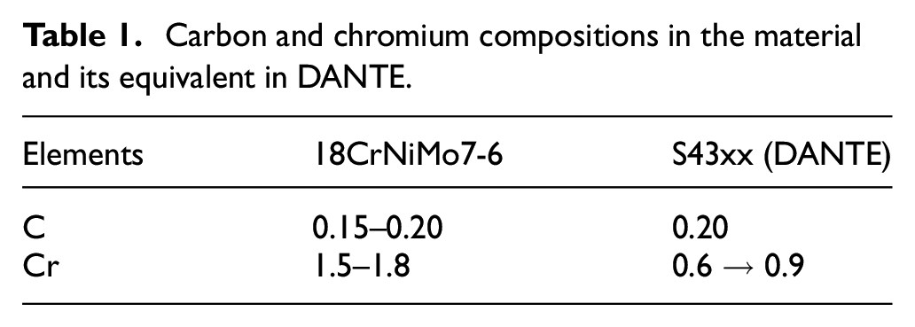
The Voith component is made of 18CrNiMo7-6, which is equivalent to the S43xx steel alloy from DANTE’s library. All alloying elements of S43xx lie in the range of those in 18CrNiMo7-6 except for the chromium content, see Table 1. DANTE permits ±50% alteration in alloying elements in its material. Thus, the chromium content can reach up to 0.9 wt.%. The 0.6 wt.% difference can still influence the material behavior, though. The complete composition of the material cannot be revealed due to the confidentiality of the work. On the other hand, 0.2 wt.% carbon is the minimum amount allowed for S43xx material from DANTE which marginally matches the upper bound of 18CrNiMo7-6 carbon content of 0.12–0.2 wt.%.

Table 1.

Carbon and chromium compositions in the material and its equivalent in DANTE.

Elements	18CrNiMo7-6	S43xx (DANTE)
C	0.15–0.20	0.20
Cr	1.5–1.8	0.6 → 0.9

In this model, residual stresses emerge only as a result of phase transformations, thus no external mechanical loadings are present. The initial phases in the material are set to 30% ferrite and 70% pearlite. The average grain size is 0.0635 mm based on ASTM-E112 standard. Throughout the heat treatment, the carbon content is kept at the material level of 0.2 wt%.

Thermal boundary conditions exist on all outer surfaces while carburization is applied only on the detailed area, see Figure 3. Carburization is initiated with a boost step followed by the diffuse step, refer to Figure 4. The carbon diffusion rate is controlled by a film coefficient set to 0.005 W/mm²·K. Note that the carbon diffusion is carried out in steady state thermal settings in ANSYS and thus the units are not matching.

Figure 3.

Surfaces for (a) carburizing and (b) heat transfer.

Figure 4.

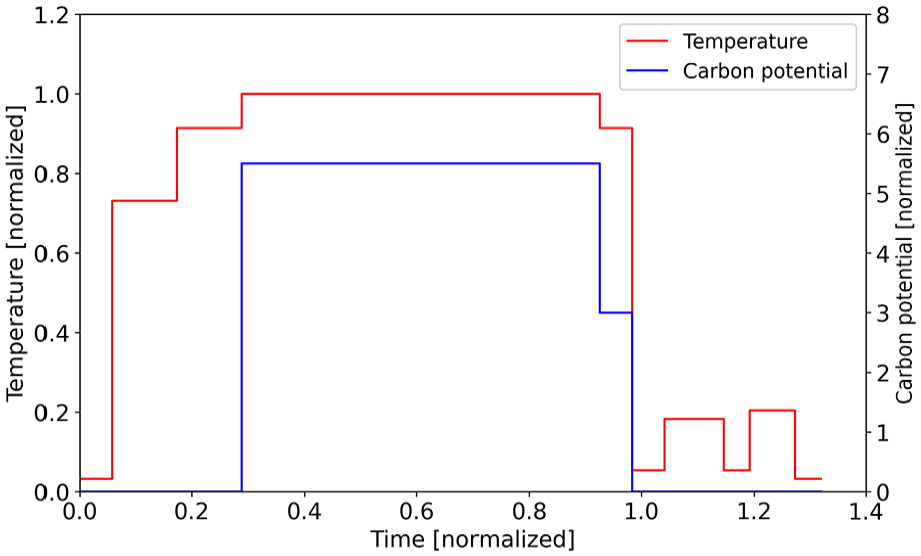
Carbon potential and temperatures.

The heat transfer coefficient (HTC) varies with respect to temperature for different heat treatment steps, namely quenching, heating, cooling, and tempering, refer to Figure 5. The values of HTCs are provided by DANTE. ¹⁷

Figure 5.

Heat transfer coefficients for (a) quenching and (b) other steps.

Additionally, Figure 6 shows the temperature-dependent Young’s modulus and Poisson’s ratio for the material model, corresponding to a base carbon content of 0.2 wt%, ¹⁸ which is present throughout most of the gear except for the carburized surface.

Figure 6.

Young’s modulus and Poisson’s ratio as a function of temperature.

Once the thermal, carburizing, and mechanical boundary as well as initial conditions are set, the model is simulated by using DANTE. Depending on the cooling rate and carbon diffusion in different depths, the volume fraction and carbon profile vary in the case and core. This is illustrated in Figure 7 (all graphs are normalized to their maximum values). The carburized surface possesses the maximum carbon weight fraction on average while the rest has the nominal value. The carburized surface depth reaches up to 8 mm in depth, see Figure 8(a) (y-axis is normalized to the base carbon). The addition of carbon shifts the bainite phase transformation curve to the right of the continuous cooling temperature (CCT) and time temperature transformation (TTT) diagrams. As a result, the amount of martensite, tempered martensite as well as the retained austenite increases in the carburized surface, see Figure 7(b) to (d), respectively. In contrary, the amount of the lower and upper bainite (Figure 7(e) and (f)) tends to increase close to the non-carburized surface and toward the core, respectively. This shows the materials high susceptibility to form bainite and thus require very high cooling rate to achieve martensite. Finally, the softer phases, namely pearlite (Figure 7(g)) and ferrite (Figure 7(f)) have highest amounts toward the core, where the cooling rate is relatively low.

Figure 7.

Normalized phase volume fractions and carbon content.

Figure 8.

(a) Carbon gradient through the case (b) total hardness.

Following the gradient of the carbon diffusion into the case (Figure 8(a)), the hardness profile follows the same pattern as presented in Figure 8(b). The hardness values are specifically maximum under the carburized surface, approximately twice as much as in the core. The non-carburized outer surfaces also demonstrate greater hardness in comparison to the core due to the intense thermal shocks experienced during quenching, coupled with the highest cooling rates in that region.

Figure 9 illustrates the normal as well as the shear residual stresses with respect to a cylindrical coordinate system, where stress values are all normalized with respect to a specific stress value through this work. The maximum compressive normal stresses reach up to −500 to −650 MPa whereas the maximum tensile ones are about 290–360 MPa. The upper left corner of the g given geometry is a stress as well as volume/weight fraction concentration as it is carburized from two neighboring surfaces. Consequently, extremely higher magnitudes of stresses and carbon are observed at this corner. The shear stresses are trivial for hoop-radial and axial-hoop directions whereas the axial-radial direction shows values varying between −180 and 200 MPa.

Figure 9.

Normalized normal and shear stresses with respect to cylindrical coordinate system: (a) Hoop stress, (b) Shear stress (hoop-radial), (c) Radial stress, (d) Shear stress (axial-radial), (e) Axial stress, and (f) Shear stress (axial-hoop).

Experiment and sensitivity analysis

Among different residual stress measurements techniques, ² only few can measure in depth residual stresses. Here, (incremental) deep hole drilling (iDHD) was applied to evaluate the stresses inside a narrow hole through the thickness of the gearbox component. To obtain a 2D stress field at different depths, first a thin cylindrical hole of 1.5–5 mm diameter is gun drilled thoroughly. The reference hole is measured in different angles at several depths by an air probe. Next, a trepan core around the reference hole is drilled using electrical discharge machining (EDM). This results in the relaxation of the reference hole. Finally, the diameters of the hole are again measured at the same positions with the air probe and the core is extracted. Changes in the diameter before and after eroding relate to the stresses in different directions based on the linear elasticity. For further information, refer to Leggatt et al. ²⁵ In case, higher plasticity effects at the cutting edges are present, incremental DHD is utilized to account for the elastoplastic effects. ²⁶

Figure 10 shows the DHD locations on the component. There are the three paths, namely P1, P2 and P3 at 800, 650 and 500 mm radii, respectively. The cylindrical coordinate system is shown on the gearbox element. Stress values are determined using the analytical solution of the axisymmetric problem using polar coordinates and Airy’s stress function (Mitchell solution). Therefore, only tangential (hoop) and radial stress components with their corresponding shear components are determined.

Figure 10.

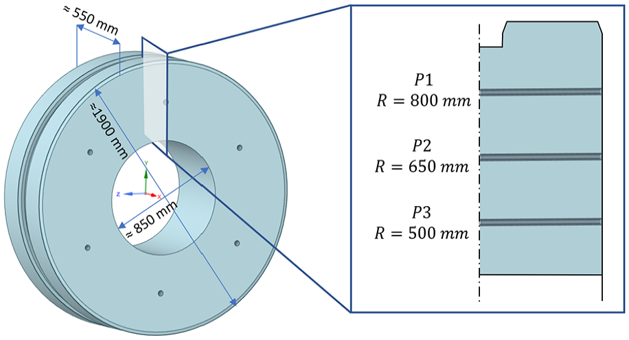
Locations for deep hole drilling (DHD) measurements.

A comparison of the measured residual stress values with the finite element (FE) results for the three paths is presented in Figure 11. Shear stresses (hoop-radial) in all three paths for both experiment and FE results are approximately zero, indicating the principal directions for the polar coordinates system. Path 1 shows good agreement for both hoop and radial stresses. The results diverge when it comes to paths 2 and 3. For the latter, numerical values of normal stresses overestimate the experimental values to a very high degree. Nevertheless, the trends remain similar. Another difference is the depth at which the compressive stresses turn to tensile ones. Experimental values show a depth closer to surface in comparison to those in the FE values.

Figure 11.

Experimental and numerical residual stress values: (a) path 1, (b) path 2, and (c) path 3.

The finite element results show deviations from DHD experimental measurements. These differences are expected due to various factors, including carburizing conditions, absence of detailed geometry consideration, shot peening, cutouts, material differences (S43xx with significant chromium content deviation) as well as HTCs. The impact of these factors on results is discussed:

1. Carburizing boundary conditions, specifically time and temperatures, influence results. Assumed conditions lead to a surface carbon content of approximately 0.7 wt.%, still in range, but may not represent the actual value, affecting phase evolutions and resulting residual stresses.

2. The omission of geometry details to save computational efforts, affects the carburized case volume and, consequently, influences residual stresses in both surface and core regions.

3. Post-treatment steps like shot peening were not included in simulations. This introduces compressive residual stresses, impacting stress variation.

4. Significant cutouts in the inner bore after the heat treatment and shot peening influence the equilibrium of residual stresses due to the removal of the material.

5. The equivalent material (S43xx) from DANTE with increased chromium content affects phase evolutions, material properties, and stress distribution, contributing to higher stresses in core in the FE calculations.

6. The assumed heat transfer coefficients (HTCs) influence the heating/cooling rates especially during quenching and can significantly affect stress development across the element.

Hardness and retained austenite values were measured at the core and 5 mm beneath the case surface in the non-carburized layer, see Figure 12.

Figure 12.

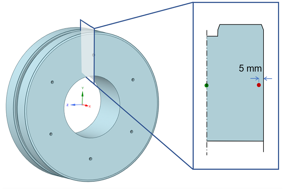
Locations for the hardness and retained austenite measurements.

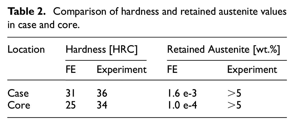
The results for both hardness and retained austenite, obtained through experiment and finite element analysis, are detailed in Table 2. Experimental findings reveal higher hardness levels compared to values derived from FE analysis at the specified locations. The FE calculations indicate significantly lower levels of retained austenite in contrast to the experimental results. These disparities might be attributed to the reduced chromium content in the FE material (S43xx) when compared to the original composition of the 18CrNiMo7-6 alloy.

Table 2.

Comparison of hardness and retained austenite values in case and core.

Location	Hardness [HRC]		Retained Austenite [wt.%]
	FE	Experiment	FE	Experiment
Case	31	36	1.6 e-3	>5
Core	25	34	1.0 e-4	>5

To shed light on the decisive factors resulting in the differences between experiment and finite element results, we focus on quench heat transfer coefficient (HTC), chromium content, and carburizing. As path 2 exhibited the highest differences and lies near the center, we focus on these results for a concise analysis.

Heat transfer coefficients control the heating/cooling rates during furnace heating, quenching, air cooling and tempering. Nonetheless, quenching is the one with the highest gradient and thus affects the residual stress the most. Therefore, we focus here solely on this process. HTCs depend on the surface temperature. Figure 13 presents this dependency for four different HTCs, namely oil A–D. These values are collected from DANTE, ¹⁸ Buczek and Telejko, ²⁷ Eshraghi et al., ²⁸ and Liščić and Filetin, ²⁹ respectively.

Figure 13.

Different heat transfer coefficients for several oils during quenching.

Figure 14 emphasizes the significant influence of the quench HTCs on the normal stress components. Specifically, Oil A shows elevated tensile residual stresses due to its increased heat extraction, resulting in higher cooling rates. Conversely, Oils B, C, and D display decreased tensile stresses in their core for all stress components, with both axial and radial stresses shifting toward a compressive state.

Figure 14.

Influence of the choice of HTCs during quenching on residual stresses along path 2: (a) hoop stress, (b) radial stress, and (c) axial stress.

As outlined in Table 1, the chromium content for the Voith actual material (18CrNiMo7-6) should fall within the range of 1.5–1.8 wt.%. This contrasts with the DANTE material (S43xx) which has a nominal chromium content of 0.6 wt.%. Consequently, a parametric investigation on the chromium content is conducted, taking into account the allowable lower and upper limits of 50%, as illustrated in Figure 15. Furthermore, the influence of the chromium content on the TTT diagrams of both materials is studied using DANTE tools.

Figure 15.

The influence of chromium content on residual stresses along path 2: (a) hoop stress, (b) radial stress, and (c) axial stress.

Figure 15 shows that with the increase in the chromium content, a decrease in all normal stresses within the core of the component occurs. However, no significant impact is evident in the case of components experiencing compressive stresses. This influence is likely attributed to the contribution of chromium content to phase evolution kinetics.

Figure 16 illustrates how changing the chromium content in the S43xx alloy (used material) and 18CrNiMo7-6 (original material) affects certain properties. Increasing chromium shifts the curves to the right and up, causing variations in results like phase changes, hardness, and stress levels at different chromium levels.

Figure 16.

Influence of chromium content on time-temperature-transformation (TTT) diagram for (a) the original material, ³⁰ 18CrNiMo7-6 and (b) S43xx. ¹⁸

To sum up, different chromium levels affect phase transformations in the case and core, leading to varied phase fractions. The summation rule for residual stress, based on contributions from all phases, results in stress variations. Notably, the core region experiences decreasing tensile stresses with higher chromium concentrations. This accounts for the disparity in stress values between the experimental and numerical results depicted in Figure 11.

Carburizing a specific part of the component’s case, known as the geometry detail, may affect the stress distribution in the core of the component. This influence was investigated through two separate simulations. The first one had no carburizing, maintaining a base carbon content of 0.2 wt.%. In the second simulation, carburizing was applied following the heat treatment sequence in Figure 4, resulting in a carburized layer depth of approximately 8 mm and a carbon content between 0.6 and 0.8 wt.%.

The results, presented in path plots and compared with experimental data in Figure 17, indicate that carburizing does affect the overall stress state in the core. This is attributed to the self-equilibrium nature of residual stresses, where the higher compressive stresses from carburizing on one face influence the tensile stresses in the core. Geometry detail is not considered in FE simulation. Instead, a planar face is used. Considering the additional surface area exposed to the carbon-rich environment due to the geometry detail, it becomes crucial to accurately determine the carbon profile of carburized layers for an overall assessment of the residual stresses. This leads to the deviation of experimental values from numerical ones, see Figure 11.

Figure 17.

Influence of carburizing residual stresses along path 2: (a) hoop stress, (b) radial stress, and (c) axial stress.

Stress mapping

When there is a need to assess residual stresses in multiple gearbox components with similar classes but varying dimensions, FEA can become a tedious and computationally expensive task. Machine learning (ML) based surrogate regression models have been found to be a suitable alternative to overcome the computational expenses. This data-driven approach reduces the time needed for stress prediction and the computational cost. For training these surrogate models, multiple FE analysis are needed to be carried out for preparing the dataset. However, the capability of ML model to predict the stress values still outperforms conventional FE techniques for a wide range of geometries.

In analogy to the FE model, we only consider a 2D half plate to predict the stress in the whole component geometry. A single class of the component with varying geometry sizes has been considered. There exists a non-linear correlation between the various dimensions. A homogenous scale factor (SF) has been introduced which describes the size of the gear wheel to overcome this non-linear correlation. The gear wheel with pitch diameter ≈1850 mm has been considered as the reference size with a scale factor of one. All the other sizes have been scaled with respect to this gear wheel size. The smallest part possesses a scale factor of 0.2. By doing such, this range of scale factors lies within the range of actual Voith gear wheel geometries with respect to various dimensional features as shown in Figure 18.

Figure 18.

(a) Real versus scaled component dimensions, (b) fitting of geometry using alpha shape.

Within the scope of this study, the heat treatment boundary conditions originate from the largest component size (SF = 1) and are assumed to be consistent across the remaining scale factors. The stress profiles for different scale factors with normalized coordinates are depicted in Figure 19. It is observed that stress magnitudes increase with increasing geometry sizes, that is, scale factor (SF).

Figure 19.

Normal stress contours for different geometry scale factors (SF).

Trends

Residual stresses in gearbox components, arising from phase transformation and thermal effects, show size-dependent behaviors. The non-linear relationships between exposed surface area (E.S.A), volume and scale factors are illustrated in Figure 20(a). As a result, different cooling rates contribute to stress differences (Figure 20(b)). Besides, components with smaller sizes reach the prescribed temperatures in the tempering processes faster. Consequently, stress relaxations are influenced. The intricate interplay of thermal gradients, phase evolution, carburizing, and tempering collectively determines the final stress state in components of varying sizes.

Figure 20.

The relationship between geometry and scale factors for (a) Exposed Surface Area (E.S.A), volume, and (b) E.S.A. to Volume ratio along with hoop stresses at three locations.

Dataset and models setup

Three machine learning models, namely Neural Network (NN), Random Forest Regression (RFR), and Support Vector Regression (SVR), were employed to predict stresses. The dataset used for model training comprised simulation data from nine scale factors ranging from 0.2x to 1x. The dataset, totaling 90,000 rows, included three input features (X, Z, SF) and six stress components as targets. Spatial datapoints, initially nodal positions, were linearly interpolated into a 100 * 100 grid for consistency. Grid points outside the geometry boundary are removed.

Figure 21 illustrates both interpolated and FE normal stress components along the predefined path. While neural network (NN) models are implemented on all six stress components, random forest regression (RFR) and support vector regression (SVR) exclusively cover the normal stress components.

Figure 21.

(a) Definition of the path and (b) comparison between interpolated and FE stress values.

Artificial Neural Networks (ANN): A grid search is employed to determine optimal parameters. Exploring configurations with 2, 3, and 4 hidden layers, activation functions (sigmoid and tangent hyperbolic), and neurons per layer (32, 64, and 128), the best model is selected based on minimizing the mean absolute error, that is, loss function. The loss versus epoch plots for each iteration in this parameter search are shown in Figure 22.

Figure 22.

ANN model: Iterations for the best parameter search.

The final model consists of one input layer and one output layer with 3 and 6 neurons, respectively, see Figure 23. Following hyperparameter optimization, the model retains three hidden layers, each comprising 128 neurons with a Sigmoid activation function as the final choice of hyperparameters. The model is compiled using the Adam optimizer and Mean Absolute Error (MAE) as the loss function. The total number of epochs is set to 500 with a batch size of 32, and 20% of the data is reserved for validation during training.

Figure 23.

Schematic view of the ANN model.

Random Forest Regression (RFR): The model employs test and train sets with an 80–20 split and a seed of 42. Features and targets are defined and scaled between −1 and 1. With default parameters (Table 3) and 100 decision trees, the model performs well, yielding reasonable predictions.

Table 3.

Hyper parameters for RFR model.

Hyper parameter	Value
Bootstrap	True
Criterion	Squared error
Max Depth	None
Max Features	1.0
Max Leaf Nodes	None
Max Samples	None
Min Impurity Decrease	0.0
Min Sample Leaf	1
Min Sample Split	2
Min Weight Fraction Leaf	0.0
Warm Start	False

Support Vector Regression (SVR): The features (X, Z, SF) and targets (Normal stress components) are defined and scaled between −1 and 1. Individual SVR models are created, and hyperparameter optimization is performed with a specified search space. The final parameters, obtained from 80 iterations, are presented in Table 4.

Table 4.

Hyper parameters for SVR model.

Hyperparameter	Optimized values
Kernel	RBF
Gamma	50
Epsilon	0.0481
Coef	1.1392
C	200

The choice of the RBF kernel is influenced by the observed non-linear relationships, particularly in X and Z coordinates. Refinement of gamma values and regularization error, impacts computational time; a range up to 0.1 is considered. The final model employs optimized hyperparameters from the defined search space.

Results

Normal stress components

Model performance is evaluated by comparing actual versus predicted stress components, see Figure 24. All models demonstrate effectiveness in predicting both test and train data. Notably, the RFR model exhibits nearly perfect predictions for each normal stress component, while the NN and SVR models display a slightly broader spread, attributed to applied regularization to prevent overfitting.

Figure 24.

Comparison of actual stress values with predictions using different regression models for both the training and testing datasets.

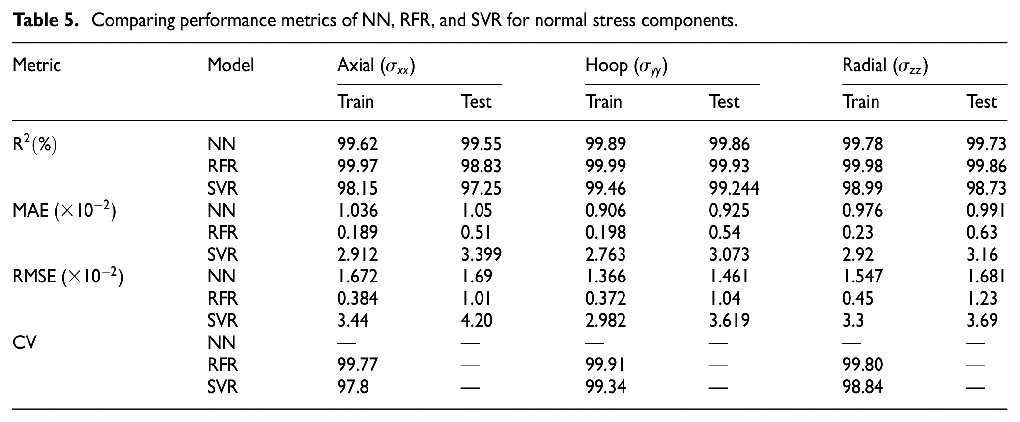
Evaluation metrics, including Root Mean Absolute Square (RMSE), Mean Absolute Square (MSE), and Coefficient of Determination (R2), serve as performance indicators. Further, 4-fold cross-validation is implemented for SVR and RFR models. Maintaining a consistent scale of features and targets between −1 and 1 for all models, the obtained scoring metrics are detailed in Table 5.

Table 5.

Comparing performance metrics of NN, RFR, and SVR for normal stress components.

Metric	Model	Axial ( ${\mathit{\sigma }}_{\mathrm{xx}}$ )		Hoop ( ${\mathit{\sigma }}_{\mathrm{yy}}$ )		Radial ( ${\mathit{\sigma }}_{\mathrm{zz}}$ )
		Train	Test	Train	Test	Train	Test
${\mathrm{R}}^2(\mathrm{\%})$	NN	99.62	99.55	99.89	99.86	99.78	99.73
	RFR	99.97	98.83	99.99	99.93	99.98	99.86
	SVR	98.15	97.25	99.46	99.244	98.99	98.73
MAE ( $\times {10}^{-2}$ )	NN	1.036	1.05	0.906	0.925	0.976	0.991
	RFR	0.189	0.51	0.198	0.54	0.23	0.63
	SVR	2.912	3.399	2.763	3.073	2.92	3.16
RMSE ( $\times {10}^{-2}$ )	NN	1.672	1.69	1.366	1.461	1.547	1.681
	RFR	0.384	1.01	0.372	1.04	0.45	1.23
	SVR	3.44	4.20	2.982	3.619	3.3	3.69
CV	NN	—	—	—	—	—	—
	RFR	99.77	—	99.91	—	99.80	—
	SVR	97.8	—	99.34	—	98.84	—

The predictive capacity of three regression models were evaluated through contour predictions for an untrained scale factor of 0.585, purposely omitted during training for validation purposes. Reference contours from finite element analysis for axial (σ _xx ), hoop (σ _yy ), and radial (σ _zz ) normal stresses are shown along with predictions from the models in Figure 25. The Neural Network model demonstrates superior performance in capturing intricate details with precision. In contrast, RFR and SVR exhibit some deviations and lower accuracy in predicting stress concentrations.

Figure 25.

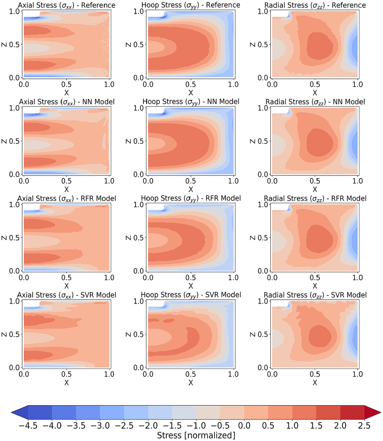
Normal stress predictions for SF = 0.585 using diverse regression models.

Residuals, the differences between actual FE reference values and predictions from regression models, serve as crucial indicators of model accuracy. These differences, calculated by subtracting predicted values from actual FE values, quantify model errors in prediction. Positive residuals indicate underestimation, while negative residuals represent overestimation. Results as shown in Figure 26 highlight the Neural Network’s minimal deviation from actual values, relatively higher deviation by the Random Forest Regression in axial and hoop stresses, and notable deviations in the Support Vector Regression. These findings pinpoint potential areas for further optimization of RFR and SVR model.

Figure 26.

Residual analysis for SF = 0.585: model accuracy between FE values and predictions.

Supplementary path plots, situated at Z = 0.5 along the x-axis, highlight the close alignment of Neural Network predictions with the reference, see Figure 27. In comparison, the Random Forest Regression (RFR) and Support Vector Regression (SVR) models display minor deviations.

Figure 27.

Normal stress: path plot at z = 0.5 for SF = 0.585 of various models.

Shear stress components

In this study, it was emphasized that among the utilized ML methods, only the ANN model is employed for predicting shear stress components. However, the performance for XY and XZ shear stress components is suboptimal. The primary challenge arises from the shear stress distribution across the plate, where stress magnitudes fluctuate around zero within a relatively narrow range. These fluctuations appear random and lack a distinct pattern, as depicted in Figure 28.

Figure 28.

Shear stresses for SF = 0.585; (upper row) actual FE, (middle row) NN predictions and (lower row) their residual analysis.

The inherent randomness poses challenges for the neural network in effectively detecting and learning from patterns on the 2D plate. Despite this, the neural network model shows more promising results for the XZ shear component, effectively recognizing patterns and yielding satisfactory predictions for both training and testing datasets, as depicted in Figure 29.

Figure 29.

Comparison of actual stress values with predictions using NN model for both the training and testing datasets.

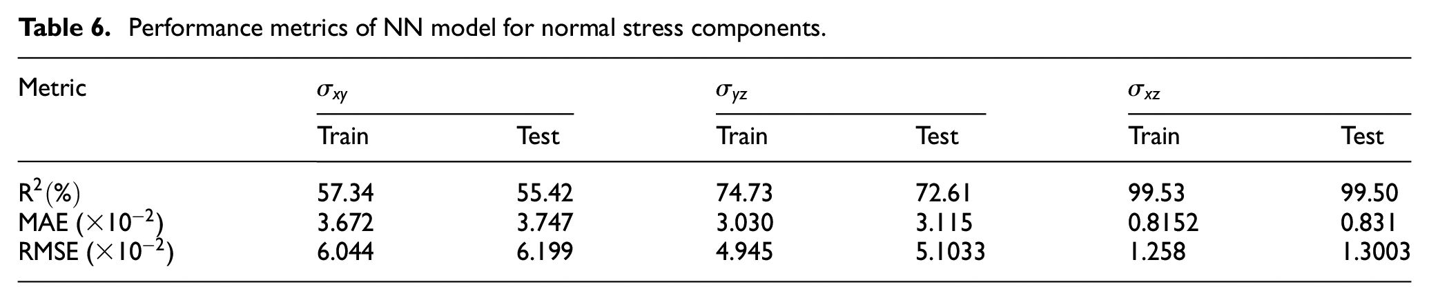
Table 6 displays scoring metrics for all shear components, underscoring the model’s suboptimal performance for stress components ${\mathit{\sigma }}_{\mathrm{xy}}$ and ${\mathit{\sigma }}_{\mathrm{yz}}$ , while delivering superior results for ${\mathit{\sigma }}_{\mathrm{xz}}$ . In analogy to the normal stress components, predictions along with their residuals for SF = 0.585 are depicted in Figure 28. The contours reveal the model’s proficiency in capturing patterns for the XZ shear component compared to the XY and YZ components. Additionally, Figure 30 illustrates reference and predicted shear stress components along a path at Z = 0.5 (path schematics in Figure 21(a)). The predicted values show a very good agreement with the reference (actual FE values) despite the mathematical differences for the shear components XY and YZ.

Table 6.

Performance metrics of NN model for normal stress components.

Metric	${\mathit{\sigma }}_{\mathrm{xy}}$		${\mathit{\sigma }}_{\mathrm{yz}}$		${\mathit{\sigma }}_{\mathrm{xz}}$
	Train	Test	Train	Test	Train	Test
${\mathrm{R}}^2(\mathrm{\%})$	57.34	55.42	74.73	72.61	99.53	99.50
MAE ( $\times {10}^{-2}$ )	3.672	3.747	3.030	3.115	0.8152	0.831
RMSE ( $\times {10}^{-2}$ )	6.044	6.199	4.945	5.1033	1.258	1.3003

Figure 30.

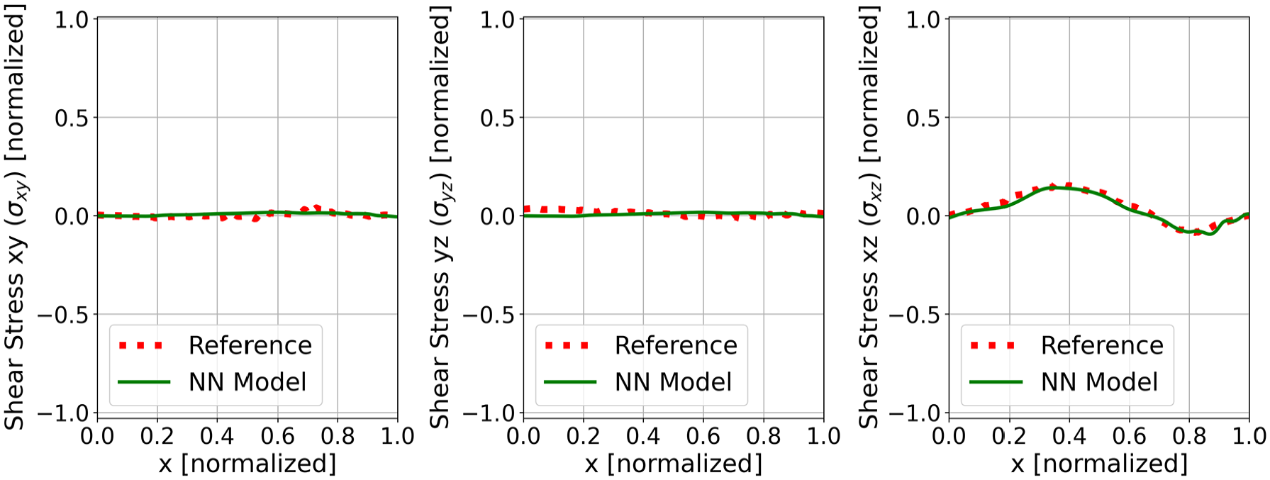
Shear stress: path plot at z = 0.5 for SF = 0.585 using NN model.

Discussion

In this comparison of residual stress prediction models, which used the same training dataset and thorough hyperparameter tuning, the ANN consistently outperformed the SVR and RFR models in terms of prediction accuracy and time. This benefit stems from the ANN’s ability to capture complex, non-linear relationships in data—relationships that cannot be adequately described using geometric dimensions alone. The ANN’s multi-layered design and activation functions allow it to capture complex patterns and interactions more precisely than SVR’s kernel-based method and RFR’s ensemble averaging, both of which struggle with the dataset’s high-dimensionality and non-linearity. This behavior is observable in prediction inaccuracies for SVR and RFR model especially for axial and hoop stress components as shown in Figure 26 and Figure 27 indicating a bias in predictions. However, it is worth noting that further refinement and fine-tuning of SVR and RFR could potentially enhance their performance. Though this process may be time-consuming and computationally expensive, it has the potential to improve their predictive accuracy.

Another benefit of the ANN is its ability to handle multi-output cases efficiently. In contrast, SVR and RFR necessitate separate models for each stress component, which significantly increases computational costs and training time. For example, training six SVR or RFR models for six stress components incurs significant overhead when compared to training a single ANN model that manages all outputs simultaneously. This capability makes the ANN ideal for predicting spatial stress distributions with multiple stress components.

Furthermore, the ANN’s flexibility enables refinement by adjusting the weight contributions to the loss function for each target variable. This feature is especially useful when working with individual geometric features, rather than a single scale factor (SF), that may have complex correlations. However, the current results show that the ANN model with refined hyperparameters is already performing well for most stress components, except for XY and YZ shear stresses, which lack observable patterns.

It is important to note that all the models used in this study are data-driven and rely on statistical correlations within the dataset, which are optimized using loss functions such as mean absolute error or mean squared error. While these models are reliable within the training data range, they may struggle when extrapolating. One improvement could be to integrating physics-informed neural networks, ¹⁵ which incorporate physics-based laws into the loss function. ¹⁶ This can potentially improve performance, particularly in extrapolation scenarios.

Summary and outlook

This study provides a concise overview of a multiphase internal state variable model. The heat treatment process of a gearbox element was simulated using finite element analysis to determine residual stress values. These were then compared with experimental data obtained through deep hole drilling of the same part. Discrepancies between the simulation and experimental results were examined, leading to the establishment of a sensitivity analysis to identify contributing factors. The investigation explored the importance of surrogate models, specifically artificial neural networks (ANN), random forest regression (RFR), and support vector regression (SVR), for mapping stress in various scaled geometries of the same material.

• The disagreements between FE and experimental results arise from factors such as carburizing conditions, geometric simplifications, material cutouts, shot peening, and the determination of material and simulation parameters.

• A correlation was observed between the geometrical scale factor, the surface area-to-volume ratio, and the resulting stress field.

• Nine finite element simulation results for different component sizes were employed in training, optimization, and analysis.

• Unlike SVR and RFR, which usually output a single target quantity and require a separate model for each stress component, artificial neural networks (ANNs) can predict the entire symmetric stress field (comprising six components) simultaneously.

• The ANN approach demonstrated superior accuracy and efficiency in predicting residual stress distributions for gear wheels ranging from pitch diameter of 350–1850 mm.

Recognizing the ongoing need for incorporating more detailed non-linear relationships, such as changes in material, can enhance the methodology to encompass a broad spectrum of non-scaled geometries within similar components. In addition, through the application of physics-informed machine learning, the need for extensive acquisition of FE data can be eliminated for the future work.