Sage Journals: Discover world-class research

Abstract

Early detection and prompt intervention by maintenance engineers to mitigate the impact of breakdowns while enhancing overall operational efficiency remain critical challenges. This study proposes an innovative approach aiming at improving the diagnosis of gear faults. The objective is to assess the sensitivity and performance of traditional indicators in comparison to cyclostationarity, examining their impact on noise levels and vibrational signatures. The initial phase involves simulating gear signals under various conditions such as amplitude, rotation frequency, and meshing frequency, providing the foundation for a thorough analysis of indicator sensitivity and performance. In the second phase, both scalar and cyclostationary indicators were calculated. First, these indicators were compared against simulated signals, and second, their sensitivity and roughness were evaluated using signals measured on the bearings of 101 BJR reducers. This approach revealed that cyclostationary indicators are more sensitive than scalar indicators, suggesting an opportunity to improve the prediction of signal roughness throughout the production process. By introducing new possibilities to enhance the reliability of vibrational measurements, this method contributes to advancing the diagnosis of gear faults.

Keywords

Scalar indicator cyclostationary indicator spectral analysis DIM IDIM simulated signals 101 BJR gearbox

Introduction

Condition-based preventive maintenance plays a crucial role in industry by extending the lifespan of rotating machines and reducing operational and maintenance costs. Vibration analysis is widely employed for defect detection and prevention. However, challenges persist regarding the accuracy and reliability of defect detection techniques, especially for gears. Significant advancements have been made in psychoacoustic roughness and cyclic roughness.¹ Essential tools of second-order cyclostationary process theory have led to the development of sensors capable of detecting and classifying common gear faults. These indicators provide information in the form of unique scalar values, simplifying their interpretation in terms of the probability of fault presence. They are also adaptable to various levels of damage, whether in stationary or non-stationary operation, and take into account uncertainties related to the characteristic frequencies of systems, which are crucial for gear diagnostics. Several studies have demonstrated the effectiveness of applying second-order cyclostationarity in the analysis of vibration signals emitted by gears.²

This approach offers improved detection and localization capabilities for gear faults, including multiple faults, thus enhancing the predictive maintenance of gears. Experimental studies have been conducted using vibrational signals to extract information related to gearbox faults. The results have clearly demonstrated the effectiveness of second-order cyclostationarity-based analysis in detecting gear faults. Therefore, vibration analysis based on second-order cyclostationarity proves to be a powerful method for detecting,³ localizing, and characterizing gear faults. This approach contributes to enhancing the reliability and accuracy of predictive maintenance for rotating machinery.

The authors conducted a study on entropy analysis using field data from two wind turbines in China.⁴ The use of entropy proves advantageous for detecting and assessing the progression of preliminary bearing faults. This method allows for a quantitative evaluation of bearings. In another study,^5,6 the authors developed a fault diagnostic method based on an integral extension of the multiscale entropy method and the least squares support vector machine method. This approach has been effective in diagnosing wind turbine faults, taking into account the non-stationary and non-linear characteristics of the vibration signal.

In the article,⁷ the authors propose a signal-processing scheme for planetary gearboxes by combining the improved Vold-Kalman filter (IVKF) and multiscale sample entropy (MSSE). They demonstrate that this method successfully identifies two types of planetary gear faults (tooth crack and distributed wear) under non-stationary working conditions. Furthermore, a new fault diagnostic framework is introduced based on a long short-term memory (LSTM) model.⁸ This method can efficiently classify faults from raw time series signals collected by one or multiple sensors, surpassing state-of-the-art approaches. Other researchers have also explored recent advances in gear fault diagnosis and prognosis.⁹ This research provides a comprehensive overview of the latest developments in gear fault diagnosis and prognosis, including methods based on machine learning and deep learning. In Ref.,¹⁰ the authors propose a method to identify and online monitor gear wear mechanisms using the second-order cyclostationary (CS2) properties of vibrational signals. This method shows promise for tracking degradation caused by fatigue pitting and other wear mechanisms. Furthermore, the use of vibration analysis to detect faults in polymer gears is explored in Ref..¹¹ The statistical indicator RMS is commonly used to detect pitting faults in polymer gears. However, a new health indicator called “weighted cyclostationary correntropy” (WCCO) is proposed to more accurately assess the degradation behavior of the gear surface over time.¹² This approach has proven to be effective in monitoring gear wear under different conditions. In Ref.,¹³ the authors develop a scheme for the optimal selection of the bandwidth of the Vold-Kalman filter, ensuring the accuracy of the offshore wind turbine condition monitoring process. Additionally, a new indicator called “TEDIS” based on transmission error (TE) is proposed to assess the severity of fatigue and predict the remaining useful life (RUL) of gears.¹⁴ A comprehensive review of the current state of research on vibration-based gear wear monitoring is presented in Ref.¹⁵ This study includes the exploration of various gear surface features, the analysis of relationships between these vibrational characteristics, and provides recommendations for future work in this field. Furthermore, in the article,¹⁶ the use of statistical parameters such as beta functions a and b for bearing fault detection is explored. However, the results demonstrate that kurtosis and crest factor are more sensitive than beta functions, highlighting the importance of choosing the appropriate fault indicators based on the application and machine characteristics. Another study aims to detect cracks in gear tooth roots by measuring their dynamic response.¹⁷ The experimental results in Ref.¹⁸ demonstrate the possibility of detecting cracks in gear tooth roots, but this method requires the prior creation of cracks through fatigue on the tooth root. In this study, two diagnostic methods, namely cepstral analysis and envelope analysis, were applied to detect gear faults operating at low speeds. Both methods proved effective, but envelope analysis complements cepstral analysis, providing a more precise diagnosis.

An analysis and numerical simulation of the behavior of a single-stage spur gear transmission are proposed in Ref.¹⁹ Cepstral analysis has shown superior effectiveness over spectral analysis in detecting localized faults. Furthermore, in Ref.,²⁰ envelope analysis and scalar indicators are used to model the impulse response of a resonance; kurtosis has proven to be a more sensitive indicator than the crest factor for detecting defects that generate periodic exciting forces. A methodology, both numerical and experimental, has been developed to identify and monitor spalling defects on gear teeth using spectral analysis, cepstral analysis, and scalar indicators.²¹ This study presents an approach to optimize the use of scalar indicators in vibrational monitoring of rotating machinery to detect defects causing impulsive forces.²² Within the scope of this study, several applications were examined, involving components such as bearings and gears, using both real and simulated data. These analyses highlighted the effectiveness of the developed autonomous diagnostic system. A preprocessing step was put in place to maintain a constant and effective statistical threshold. These indicators were specifically designed to be used in an autonomous process, allowing differentiation between different types of defects within the machinery. Researchers have developed a methodology similar to that presented in the previous article²³ to optimize the use of scalar indicators in vibrational monitoring of rotating machinery for detecting defects causing impulsive forces.²⁴

In article,²⁵ an application of cepstral analysis in studying gear vibrations is presented. This study highlights the relationship between cepstral resolution and signal characteristics, providing valuable insights for gear vibration analysis. In articles,^26,27 the authors describe a technique that combines wavelet-based multiresolution analysis and the Hilbert transform to predict gear tooth defects from vibration data. This approach has shown promising results in detecting and predicting gear tooth defects in real-world applications. Additionally, a blind source separation technique based on prior knowledge of the number of independent sources present in the mixture is discussed in these articles, representing a significant advancement in the field of vibration analysis and mechanical fault diagnosis. In these articles, researchers explored various approaches to solve the problem of detecting cyclostationary signals of interest, even in the absence of prior knowledge of the number of sources. They employed techniques like subspace decomposition and cyclostationary analysis. To tackle this complex challenge, they introduced a method known as distribution intensity modulation (DIM), which is discussed in detail in related statistical studies.^28,29 Furthermore, a specific method for extracting second-order cyclostationary components from vibration signals has been developed.³⁰ This method allows for the estimation of the amount of energy associated with each cyclical component of interest in the frequency domain, which proves particularly useful for monitoring the behavior of rotating machines operating at different loads and speeds. These advancements contribute to improving the accuracy and reliability of condition-based preventive maintenance.

In article,³¹ two diagnostic methods are evaluated: phase demodulation analysis and time-frequency analysis. These methods aim to overcome the limitations of existing approaches, especially in the presence of significant variations in rotation speed or variable spectral characteristics. Furthermore, in article,³² a new method for detecting modulation in vibro-acoustic signals emitted by rotating machinery is introduced. In articles,^33,34 a new indicator called “spectral kurtosis” (SK) is proposed, designed to detect and characterize non-stationary signals. It has been demonstrated that this indicator is effective for monitoring the vibrational condition of rotating machinery. Additionally, in articles,^35,36 another innovative technique for detecting modulation in vibro-acoustic signals produced by rotating machinery is introduced. Machines inevitably produce vibrations, which can lead to wear and eventual component failure. Vibration analysis is crucial for detecting defects, particularly in gears and bearings, and plays a key role in enabling proactive maintenance. Most studies focus on reviewing condition-based maintenance (CBM) techniques and propose methods to enhance defect detection by removing transfer function effects from vibration signals. One such method was validated on a gearbox with a tooth crack, demonstrating improved defect localization.^37,38 In article³⁹ presents various signal processing methods for monitoring and diagnosing systems using acoustic and vibrational measurements. Among these methods are cyclostationary analysis and methods based on higher-order statistics. Finally, article¹⁵ focuses on the study of failures and condition-based maintenance methods for a turbo-alternator using spectral analysis and cyclostationarity. The study results highlight the effectiveness of spectral analysis and cyclostationarity in detecting various types of faults in rotating machinery. These methods contribute significantly to condition-based preventive maintenance by enabling early detection of issues, preventing costly breakdowns, and extending the lifespan of industrial equipment.⁹ Furthermore, they contribute to reducing maintenance costs by planning interventions more accurately and avoiding unplanned production downtime. This underscores the ongoing importance of research and development in the field of rotating machinery monitoring for the industry.

The cyclostationarity approach indeed plays a crucial role in monitoring and detecting anomalies in rotating machinery. The vibrations it analyzes provide critical information for assessing the health and wear of these machines. One of the major advantages of the cyclostationarity method is its user-friendliness for maintenance technicians or engineers who may not necessarily be experts in signal processing.⁴⁰ It relies on band-pass filtering and decomposition techniques, making it a powerful method for detecting mechanical faults based on previously acquired knowledge. In summary, it contributes to improving the efficiency and accuracy of diagnosis, which is essential for successful preventive maintenance.

The development of new vibrational and cyclostationary indicators is crucial to enhance the reliability and performance of condition-based preventive maintenance. These technological advancements allow companies to optimize their operations by extending the lifespan of rotating machinery while reducing maintenance costs. Moreover, they contribute to ensuring increased machine availability and enhanced industrial process efficiency. By investing in the research and development of these technologies, businesses can improve their competitiveness and maintain their assets in a more cost-effective manner.

Sampling and scanning techniques

To apply a calculation algorithm, it is essential to digitize the signal through an analog-to-digital converter at a sampling frequency denoted as $F_{s}$ _sample. The spectrum computation is performed over a specified number of $N_{e}$ _samples, with a time interval Δt corresponding to $\frac{N_{e}}{F_{s}}$ for each block of $N_{e}$ _samples utilized in the spectrum calculation. The theoretical spectrum is calculated over sample points or spectral lines, but contemporary analyzers typically display only $\frac{N_{e}}{2.56}$ spectral lines in practice.⁴¹ If the maximum displayed frequency (F_max) is known, the sampling frequency (f sampling) is determined by:

f_{sampling} = 2.56 * F_{\max}

(1)

Gaussian white noise

Gaussian white noise, generated using the randn () function in Matlab©, is a widely employed random function to model noise in signals. Its popularity stems from its random characteristics and consistent power spectral density across all frequencies. The amplitude of the generated noise, represented as B (t), is commonly adjusted using a multiplier coefficient denoted as B_r.

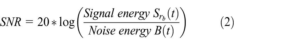
To quantify the extent of noise in a signal, the signal-to-noise ratio (SNR) is frequently employed. This ratio is computed using the following formula⁴²:

SNR = 20 * \log (\frac{Signal energy S_{r_{b}} (t)}{Noise energy B (t)})

(2)

Numerical modeling and simulation of double gear defects and scalar indicator calculation

This study aims to compare the vibrational response of gears with and without noise to understand the influence of noise on the sensitivity of scalar indicators. Utilizing a MATLAB program, we model and simulate vibrational signals in the presence of single and/or double defects, incorporating white noise into these signals. The vibrational response of the gears is then analyzed using scalar indicators, including RMS, FC, VC, K, and entropy, both before and after the introduction of noise. Examining the vibrational response of gears in the presence of defects with and without noise contributes to evaluating the efficacy of fault analysis and diagnostic methods.

Our investigation further delves into the impact of various simulation parameters on the vibrational response of gears with defects. This includes scrutinizing factors such as meshing frequencies, rotational frequencies, and amplitudes. Finally, we will conduct a comparative analysis of the vibrational response of gears with defects, considering both scenarios with and without noise. This comparative study aims to elucidate the influence of noise on the sensitivity of the indicators.

A MATLAB program is utilized to model and simulate a signal with single and double defects using trigonometric functions. Subsequently, white noise is introduced to this signal, and the signal, along with its spectrum and envelope spectrum, is visualized both before and after the noise addition. Scalar indicators are also calculated before and after incorporating the noise. Simulation parameters, including gear frequencies (F_m1, F_m2), rotational frequencies (F_r1, F_r2), and defect amplitudes (A4, A5, A11, B11, A12, B12, A13, B13), are predefined at the beginning of the program.

✓ The single defect is modeled as follows:

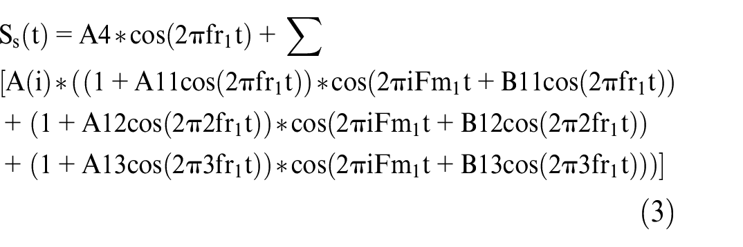
\begin{array}{l} S_{s} (t) = A 4 * \cos (2 π {fr}_{1} t) + \\ \sum [A (i) * ((1 + A 11 \cos (2 π {fr}_{1} t)) * \cos (2 π {iFm}_{1} t + B 11 \cos (2 π {fr}_{1} t)) \\ + (1 + A 12 \cos (2 π 2 {fr}_{1} t)) * \cos (2 π {iFm}_{1} t + B 12 \cos (2 π 2 {fr}_{1} t)) \\ + (1 + A 13 \cos (2 π 3 {fr}_{1} t)) * \cos (2 π {iFm}_{1} t + B 13 \cos (2 π 3 {fr}_{1} t))] \end{array}

(3)

The double defect is modeled by:

\begin{matrix} S_{c} (t) = A 4 * \cos (2 π f r_{1} t) + A 5 * \cos (2 π f r_{2} t) \\ + (1 + A 12 \cos (2 π 2 f r_{2} t)) * \cos (2 π jF m_{2} t + B 12 \cos (2 π 2 f r_{2} t)) \\ + (1 + A 13 \cos (2 π 3 f r_{2} t)) * \cos (2 π jF m_{2} t + B 13 \cos (2 π 3 f r_{2} t)))] \end{matrix}

(4)

Study of the influence of fault amplitudes on scalar indicators and vibration signature

In the initial scenario, three distinct cases are investigated. In each case, fault amplitudes are increased while keeping gear frequencies (F_m1 = 600 Hz, F_m2 = 800 Hz) and rotational frequencies (F_r1 = 15 Hz, F_r2 = 7 Hz) constant. This approach allows for a comprehensive examination of the impact of fault amplitude on the signal and its spectrum (see Table 1), with other parameters held constant to ensure accurate comparisons. The goal is to gain insights into how variations in fault amplitudes influence the detection and diagnosis of issues within the signal.

Table 1.

Fault amplitude values for “Case 1.”

A4	A5	A11	B11	A12	B12	A13	B13
0	0	5	0.25	2	0.25	1	0.25

A. Study of the influence of fault amplitudes on scalar indicators

By analyzing the data presented in Table 2, the following conclusions can be drawn:

Table 2.

Variations in indicators with changes of amplitude.

Case 1	RMS	FC	VC	K	Entropy
Noise-free	5.0033	5.7515	28.7767	5.0811	−8.8416e+05
With noise	7.1021	4.4313	31.4714	3.4838	−1.9547e+06

Increasing the defect amplitudes (A4, A5, A11, B11, A12, B12, A13, and B13) results in higher values of RMS and VP for the signal, accompanied by an increase in power entropy (entropy). Concurrently, there is a reduction in kurtosis (K) and crest factor (CF).

The introduction of noise to the signal leads to an elevation of both the root mean square (RMS) and peak value (VP), along with an increase in entropy. Meanwhile, there is a slight decrease in CF and K.

B. Study of the influence of fault amplitudes on the vibration signature

In Figure 1(a), a noise-free time-domain signal is depicted, illustrating a simulated double gear fault. Figure 1(b) displays the spectrum of this signal, distinctly revealing two gear mesh frequency modulations (F_m1 = 600 Hz and F_m2 = 800 Hz) generated by the rotational frequencies (F_r1 = 15 Hz for the input shaft carrying the pinion and F_r2 = 7 Hz for the output shaft carrying the wheel). These frequency modulations indicate the presence of two individual faults, one on the pinion and the other on the wheel.

Figure 1.

Gear double fault signal: (a) gear meshing signal without noise, (b) its spectrum, and (c) its envelope spectrum “Case 1.”

In Figure 1(c), the envelope spectrum of the signal provides additional confirmation of the existence of both rotation frequencies (F_r1 and F_r2), along with their harmonics. This verification strengthens the evidence of the two individual faults, one on the pinion and the other on the wheel. The envelope spectrum plays a crucial role in accentuating these features, thereby contributing to a more distinct detection and characterization of the faults.

By introducing Gaussian white noise to the signal depicted in Figure 1(a), the resulting signal is shown in Figure 2(a), along with its spectrum in Figure 2(b), and its envelope spectrum in Figure 2(c).

• The observations made are as follows:

Figure 2.

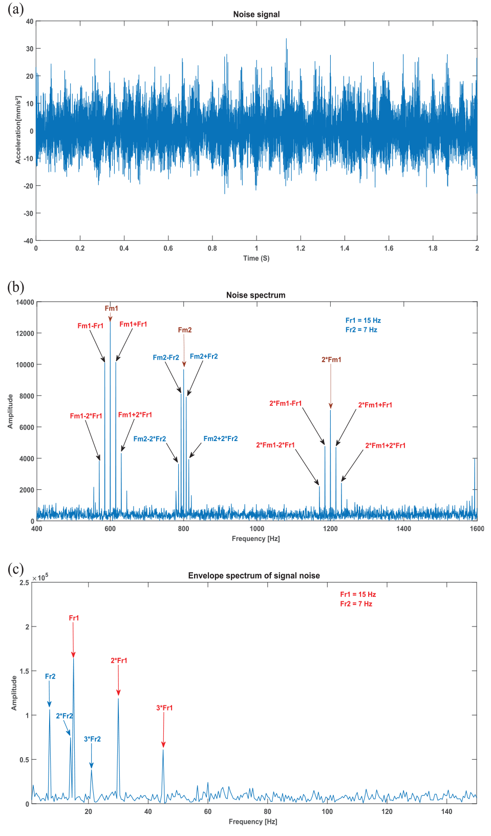
Gear double fault signal: (a) gear meshing signal with noise, (b) its spectrum, and (c) its envelope spectrum “Case 1.”

Increasing the amplitude of defects (A4, A5, A11, B11, A12, B12, A13, and B13) results in:

➢ An escalation in the amplitudes of meshing frequencies (F_m1 and F_m2) and rotation frequencies (F_r1 and F_r2), intensifying the severity of the defects and indicating a larger simulated defect size.

➢ The envelope spectrum of the simulated signal distinctly highlights the misalignment phenomenon, which may not be as noticeable in the traditional spectrum. This suggests that envelope spectrum analysis could be more sensitive for detecting specific defect characteristics, such as misalignment.

➢ The introduction of noise amplifies the amplitudes of defects and influences scalar indicators like RMS, kurtosis (K), and crest factor (CF). This rise in defect amplitudes due to noise can complicate defect detection and diagnosis, as it has the potential to obscure or magnify certain undesirable signals.

These observations underscore the importance of considering defect amplitude, noise, and the selection of indicators in signal analysis for defect detection and characterization in gear systems.

Study of the influence of rotation frequencies on scalar indicators and vibration signature

Three different cases are investigated. In each case, the rotation frequencies are incremented (see Table 3), while maintaining constant gear frequencies (F_m1= 600 Hz, F_m2 = 800 Hz) and fixed defect amplitudes (A4 = 0, A5 = 0, A11 = 5, B11 = 0.25, A12 = 2, B12 = 0.25, A13 = 1, and B13 = 0.25).

Table 3.

Rotation frequency values for each case.

Rotation Frequency	Fr₁	Fr₂
Case 2	30 Hz	Hz

A. Study of the influence of rotation frequencies on scalar indicators

By analyzing the data presented in Table 4, the following conclusions can be drawn:

➢ Introducing noise to the signal results in an elevation of the RMS and peak value (VP), along with an increase in power entropy (entropy), while the kurtosis (K) and crest factor (CF) experience a slight decrease.

➢ In the absence of noise, the values of RMS, CF, and K remain constant at 5, 5.8, and 5 Hz, respectively.

✓ In the presence of noise, the values of RMS, CF, and K stabilize at 7, 4.5, and 3.5 Hz, respectively.

✓ These observations underscore the influence of noise on scalar indicators, revealing that noise contributes to higher RMS, VP, and entropy values but lower K and CF values when compared to the noise-free scenario.

Table 4.

Scalar indicators for case 2.

Case 2	RMS	FC	VC	K	Entropy
Noise-free	5.0033	5.7515	28.7767	5.0811	−8.8416e+05
With noise	7.1021	4.4313	31.4714	3.4838	−1.9547e+06

B. Study of the influence of rotation frequencies on the vibration signature

In this scenario, the rotation frequencies are held constant at F_r1 = 15 Hz and F_r2 = 7 Hz.

Figure 3(a) presents a noise-free time-domain signal depicting a simulated double gear fault, while Figure 3(b) displays the spectrum of the noise-free signal. It clearly illustrates the two modulation frequencies F_m1 = 600 Hz and F_m2 = 800 Hz, generated by the rotation frequencies F_r1 = 30 Hz and F_r2 = 22 Hz for the input shaft carrying the pinion and the output shaft carrying the wheel, respectively. This indicates the presence of two faults, one on the pinion and one on the wheel. Figure 3(c) exhibits the envelope spectrum of the noise-free signal, revealing the presence of both rotation frequencies F_r1 and F_r2 along with their harmonics, confirming the existence of two faults. Additionally, it distinctly highlights the presence of an alignment fault.

Figure 3.

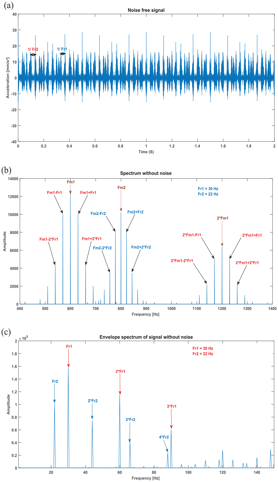
Signal of a double gear fault: (a) meshing signal without noise, (b) its spectrum, and (c) its envelope spectrum “Case 2.”

By introducing Gaussian white noise to the signal from Figure 3(a), the resulting signal is shown in Figure 4(a), accompanied by its spectrum in Figure 4(b) and envelope spectrum in Figure 4(c).

Figure 4.

Signal of a double gear fault: (a) meshing signal with noise, (b) its spectrum, and (c) its envelope spectrum “Case 2.”

Study of the influence of meshing frequencies on scalar indicators and vibration signature

We investigate three different cases. In each case, the values of gear mesh frequencies Fm₁ and Fm₂ are incremented (see Table 5), while maintaining constant rotation frequencies Fr₁= 15 Hz, Fr₂= 7 Hz, and fixed defect amplitudes (A4 = 0, A5 = 0, A11 = 5, B11 = 0.25, A12 = 2, B12 = 0.25, A13 = 1, B13 = 0.25).

Table 5.

The meshing frequency values for each case.

Meshing frequency	Fm₁	Fm₂
Case 3	4096 Hz	Hz

A. Study of the influence of meshing frequencies on scalar indicators

By analyzing the case presented in Table 6, we can conclude the following:

Table 6.

Scalar indicators for case 3.

Case 3	RMS	FC	VC	K	Entropy
Noise-free	5.1318	4.7768	24.5135	5.9507	−9.7631e+05
With noise	7.2075	4.4440	32.0298	3.8876	−2.0530e+06

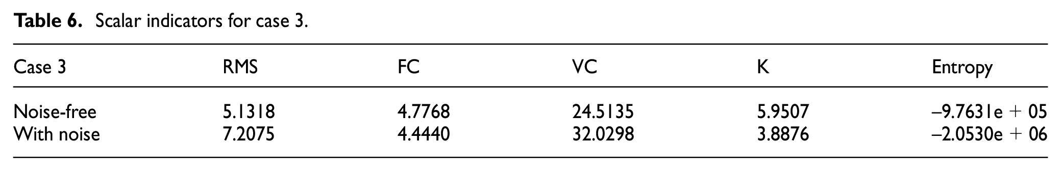
➢ The introduction of noise to the signal results in an increase in RMS and VP of the signal while decreasing K and power entropy, with CF experiencing a slight decrease.

➢ Noise amplifies the amplitudes of gear mesh frequencies and influences scalar indicators such as RMS, kurtosis (K), and crest factor (CF). In the presence of noise, these indicators can be distorted, potentially leading to erroneous interpretations of the severity levels of defects.

B. Study of the influence of meshing frequencies on the vibration signature

In this specific case, the meshing frequencies are fixed at values of Fm₁ = 4096 Hz and Fm₂ = 8192 Hz. Figure 5(a) exhibits a noise-free time signal representing a simulated double gear fault. In Figure 5(b), the spectrum of the signal without noise is presented, clearly displaying two modulations of the meshing frequency (Fm₁ = 4096 Hz and Fm₂= 8192 Hz). These modulations are generated by the rotation frequencies (Fr₁ = 15 Hz for the input shaft carrying the pinion and Fr₂ = 7 Hz for the output shaft carrying the wheel), indicating the presence of two individual defects, one on the pinion and the other on the wheel.

Figure 5.

Signal of a double gear fault: (a) meshing signal without noise, (b) its spectrum, and (c) its envelope spectrum “Case 3.”

Figure 5(c) illustrates the envelope spectrum of the signal without noise. This envelope spectrum reveals the presence of the two rotation frequencies, Fr₁ and Fr₂, as well as their harmonics. This confirmation further supports the presence of two defects, one on the pinion and the other on the wheel. When Gaussian white noise is added to the signal shown in Figure 5(a), the resulting signal can be observed in Figure 6(a). Additionally, the spectrum of this noisy signal is represented in Figure 6(b), while its envelope spectrum is displayed in Figure 6(c).

Figure 6.

Signal of a double gear fault: (a) meshing signal with noise, (b) its spectrum, and (c) its envelope spectrum “Case 3.”

The introduction of Gaussian white noise facilitates the analysis of how its presence affects both the frequency content of the signal and its envelope spectrum. These considerations are crucial when dealing with real-world data and the detection of faults or anomalies in signals.

➢ Observation for Analysis

In conclusion, the thorough mathematical modeling of a specific type of defect and the simulation of a gear fault have enabled the examination of how defect amplitudes, rotation frequencies, and meshing frequencies impact the vibration signature and scalar indicators. The key findings from this study are as follows:

➢ Altering fault amplitudes corresponds to an increase in the simulated fault’s size and severity.

➢ The amplification of amplitudes in both the meshing frequencies (Fm₁ and Fm₂) and the rotation frequencies (Fr₁ and Fr₂) impacts the severity of the defects, resulting in an increase in the simulated defect’s size.

➢ The envelope spectrum of the simulated signal effectively reveals the misalignment phenomenon, which is not readily apparent in the standard spectrum.

➢ Adding noise increases defect amplitudes and impacts scalar indicators such as RMS, kurtosis (K), and crest factor (CF). The kurtosis (K) values of approximately 3 Hz and the crest factor (CF) values of approximately 3 and 4 Hz do not provide reliable information on the presence of the fault. In the presence of noise, these indicators can be distorted, leading to erroneous interpretations of fault severity levels.

➢ When there is a variation in rotation frequencies, introducing noise to the signal leads to an increase in the RMS and peak value (VP) of the signal, along with an elevation in entropy. However, there is a slight decrease in kurtosis (K) and crest factor (CF). Specifically, kurtosis (K) maintains values of approximately 5 Hz both in the absence and presence of noise, while crest factor (CF) shows values of approximately 3 Hz without noise and approximately 4 Hz with noise.

➢ When meshing frequencies are altered, introducing noise to the signal leads to an increase in RMS and peak value (VP) of the signal. However, it results in a decrease in kurtosis (K) and entropy, with a slight decrease in crest factor (CF).

The presence of meshing frequencies generated by the interaction of wheel and pinion teeth can pose a challenge in spectral analysis. These meshing frequencies can mask or obscure individual rotational frequencies, making it difficult to distinguish and isolate the specific rotational frequencies associated with the wheel and pinion when significant meshing frequencies are present in the signal spectrum. This interference can complicate the identification and characterization of other vibration components and defects within the mechanical system.

In summary, this study underscores the significance of considering defect amplitudes, rotational frequencies, and meshing frequencies when conducting vibration analysis of gears. Additionally, it emphasizes the impact of noise on scalar indicators and the challenges associated with distinguishing individual frequencies when substantial meshing frequencies are present. These insights are valuable for understanding and improving diagnostic capabilities in the context of gear fault detection and analysis.

Cyclostationarity analysis: Theory, indicators, and applications

In this section, we aim to provide a thorough understanding of the cyclostationary method, focusing specifically on its theoretical foundations, indicators, and industrial applications. Our discussion will be organized as follows:

➢ Theoretical Bases of Cyclostationary Method

Explanation of key concepts and principles that underlie the cyclostationary method.

➢ Cyclostationary Indicator

Examination of the indicators associated with cyclostationary analysis, which enable the extraction and quantification of periodicities within signals.

➢ Practical Applications of Cyclostationary Analysis

Exploration of real-world applications of the cyclostationary method, with a detailed examination of its effectiveness, including examples from simulated signals.

By covering these aspects, we aim to provide a comprehensive insight into the cyclostationary method and its relevance in industrial settings for signal analysis and fault detection.

Cyclostationarity is an approach that primarily utilizes the distribution intensity modulation (DIM) function to detect and characterize variations within a signal. Initially developed for diagnosing faults in various applications, including gears, rolling and plain bearings, and telecommunication signals, the spectral correlation density method focuses on identifying amplitude variations characterized by symmetrically spaced sidebands in spectra. This approach enables the visualization of modulation indicator values on a frequency graph, which is a function of both the carrier frequency (f) and the modulation frequency (α) of the signal.

When the signal is filtered in this way, in an idealized case, it contains only the specified component without any additional signal and with a very low noise level. Thus, the filtered signal is composed of a set of three elements:

x_{i} = x_{Δ f} (t; f - i α) with i = {- 1, 0, 1}

(5)

x_i represents a single value of the signal, $x_{Δ f} (t, f)$ indicates the filtered version of x(t) in a side frequency band $[f - \frac{Δ f}{2}; f + \frac{Δ f}{2}]$ with Δf being the step frequency.

In this context, when we mention that $x_{Δ f} (t, f)$ represents a single value of the signal, we mean that $x_{Δ f} (t, f)$ is a specific value or data point within the filtered signal. This value is obtained by filtering the original signal x(t) in a specific frequency range or band, denoted as $[f - \frac{Δ f}{2}; f + \frac{Δ f}{2}]$ , where Δf represents the frequency step.

So, $x_{Δ f} (t, f)$ is the representation of the signal x(t) after it has been filtered to isolate the frequency component within the specified band $[f - \frac{Δ f}{2}; f + \frac{Δ f}{2}]$ . This filtered signal value at time t and frequency f is a result of the filtering process and reflects the signal’s characteristics within that particular frequency range.

In Figure 7, a diagram illustrates the method used with an open functionality model for a specific statistical function. This function is responsible for calculating the spectral correlation intensity factor by defining a filter interval [a₁, a₂]. The results of the last step of the procedure include two types of indicators: the spectral correlation density (SCD) and its corresponding integration (IDIM) for a determined frequency range.

Figure 7.

Proposed algorithm for calculating classical, cyclostationary, DIM and IDIM indicators.

We can see that symmetric filtering is conditioned by three parameters: f_s, α, and Δf. The spectral correlation density of the SCD analysis frequency range is carried out as follows:

f_{min} = \frac{α_{min}}{2} + \frac{Δ f}{2},

(6)

And

f_{max} = \frac{f_{s}}{2} - \frac{α_{max}}{2} - \frac{Δ f}{2},

(7)

Where f_s is the sampling frequency of the measured signal.

The proposal of the frequency f, for a given Δf, is called the distribution intensity modulation (DIM) which can be expressed by:

DIM (f; α) = {SC}_{x}^{α} (f + \frac{α}{2}) {SC}_{x}^{α} (f - \frac{α}{2}),

(8)

The PSC index designates the product of the spectral correlation.

The degree of cyclostationarity is a measure of the energy ratio between the cyclic and non-cyclic components of a stationary signal. Its mathematical expression is given by:

DS C^{α} = \int {| R_{x}^{α} (α) |}^{2} d α / {| {SC}_{x}^{0} (α) |}^{2} d α

(9)

Using spectral correlation, it is possible to reformulate expression (9).

DS C^{α} = \int {| {SC}_{x}^{α} (α) |}^{2} df / {| {SC}_{x}^{0} (α) |}^{2} df

(10)

In some practical applications of DIM for vibrational signals, the product of spectral correlation densities, such as distribution intensity modulation, might not be the most useful measure due to large differences in signal energy across different frequency bands. In such cases, interpreting DIM plans can be more efficient when the absolute value of the spectral correlation density is normalized to vary only between 0 and 1. For this purpose, the proposed ${DIM}_{Δ f}^{PSC}$ can be extended to use the coherence spectral density as a distribution intensity modulation. The spectral coherence distribution density modulation function is obtained by³:

\begin{matrix} {DIM}_{Δ f}^{PSCoh} (f, α) = \\ (\frac{{SC}_{x}^{α} (f + α / 2)}{\sqrt{{SC}_{x}^{0} (f + α / 2)} {SC}_{x}^{0} (f)} \frac{{SC}_{x}^{α} (f - α / 2)}{\sqrt{{SC}_{x}^{0} (f - α / 2)} {SC}_{x}^{0} (f)}) \end{matrix}

(11)

The distribution density modulation of (DIM) represents the spectral correlation density, expressed by different sources, is called (IDIM). This integration will be selected over the entire band of carrier frequencies defined by²⁷:

{DIM}_{f_{1}}^{f_{2}} (α; Δ f) = \int_{f_{1}}^{f_{2}} DI M_{Δ f} (f; α) df

(12)

Where $DI M_{Δ f} (f; α)$ is a vector calculated in the carrier frequency band from f₁ to f₂.³⁴

Cyclostationary indicators

The psychoacoustic roughness and cyclic roughness indicators, which measure the roughness of the signal, can be used in fault detection through the integrated spectral coherence and spectral coherence via cyclic roughness (equations (13) and (14)), respectively. These indicators facilitate fault characterization, early detection, and severity assessment. They can be computed using the following equations^43,44:

γ_{x}^{2} (α_{l}, f_{k}) = \frac{| S_{X} (α_{l}, f_{k}) |^{2}}{S_{X} (0, f_{k}) S_{X} (0, f_{k})}

(13)

I = \frac{1}{F_{1} F_{2}} (\sum_{l, k} γ_{x}^{2} (α_{l}, f_{k})) . g (f_{k})

(14)

With: $γ_{x}^{(2)}$ represents the spectrum of the signal, $g (f_{k})$ is the weighting function for each frequency f and $(α_{l}, f_{k})$ is the autocorrelation coefficient between the indices l and k.

F₁ and F₂: are the lower and upper limits of the integration frequency range, respectively.

$γ_{x}^{(2)} (α_{l}, f_{k})$ : Rapid estimation of spectral coherence across frequency orders.

I: The Number of summed frequencies.

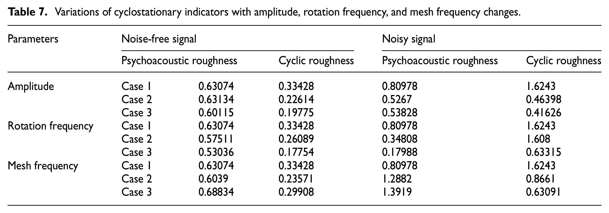
The results of the interpretations of Table 7 highlight variations in cyclostationary indicators based on different simulation parameters.

In the first case, as shown in Table 7, the “psychoacoustic roughness” indicator increases in the presence of noise, rising from 0.63 to 0.81 Hz. Similarly, the “cyclic roughness” indicator exhibits an increase in its values with the introduction of noise, going from 0.33 to 1.62 Hz.

In the second case, presented in Table 7, the “psychoacoustic roughness” indicator decreases in the presence of noise, dropping from 0.58 to 0.35 Hz, while the “cyclic roughness” indicator increases, ranging from 0.26 to 1.61 Hz.

Finally, in the third case described in Table 7, the “psychoacoustic roughness” indicator experiences a decrease in the presence of noise, decreasing from 0.69 to 1.39 Hz, while the “cyclic roughness” indicator shows an increase, going from 0.29 to 1.63 Hz. These variations underscore the impact of noise on cyclostationary indicators.

Table 7.

Variations of cyclostationary indicators with amplitude, rotation frequency, and mesh frequency changes.

Parameters	Noise-free signal			Noisy signal
	Psychoacoustic roughness		Cyclic roughness	Psychoacoustic roughness	Cyclic roughness
Amplitude	Case 1	0.63074	0.33428	0.80978	1.6243
	Case 2	0.63134	0.22614	0.5267	0.46398
	Case 3	0.60115	0.19775	0.53828	0.41626
Rotation frequency	Case 1	0.63074	0.33428	0.80978	1.6243
	Case 2	0.57511	0.26089	0.34808	1.608
	Case 3	0.53036	0.17754	0.17988	0.63315
Mesh frequency	Case 1	0.63074	0.33428	0.80978	1.6243
	Case 2	0.6039	0.23571	1.2882	0.8661
	Case 3	0.68834	0.29908	1.3919	0.63091

Application of cyclostationary analysis to simulated signals

The processing of the simulated signals presented in the section above included various aspects such as amplitudes, rotation frequencies, meshing frequencies, and different scenarios. The spectral analysis conducted allowed us to observe a substantial evolution or influence of the amplitudes on the rotation and meshing frequencies. To validate this outcome, we applied the cyclostationarity method to the simulated signals.

A. Case 1: Fault amplitudes and varying fault amplitudes with noise

The application of DIM to a simulated signal without noise was investigated. In Figure 8(a), two distinct cyclic frequencies are observed. The first fundamental cyclic frequency, α₂= 3.418 × 10⁻³*f_s ≈ 14 Hz (with f_s = 4096 Hz), is accompanied by multiple harmonics, corresponding to twice the rotation frequency of the pinion (2 × Fr₂). The second cyclic frequency, α₁= 7.324 × 10⁻³*f_s≈ 30 Hz (with f_s = 4096 Hz), has a significantly higher amplitude and is also accompanied by harmonics, corresponding to twice the rotation frequency of the wheel (2 × Fr₁). Additionally, a carrier frequency at 1200 Hz, corresponding to the second harmonic of the meshing frequency Fm₁ (600 Hz) and its harmonics, as well as a carrier frequency at 1600 Hz, corresponding to the second harmonic of the meshing frequency Fm₂ (800 Hz), are observed.

Figure 8.

(a) Spectral correlation (DIM), (b) its integration (IDIM) applied to the signal of Figure 1(a).

The use of IDIM, as illustrated in Figure 8(b), enables a clearer identification of the fundamental cyclic frequencies α₂ = 14 Hz (2 × Fr₂) and α₁ = 30 Hz (2 × Fr₁) and their harmonics. This phenomenon corresponds to a wear defect on both the wheel and the pinion, in addition to alignment issues.

The application of DIM to a simulated signal with noise was examined. Figure 9(a) reveals the emergence of two cyclic frequencies: the first, α₂ = 1.708 ×10⁻³*f_s ≈ 7 Hz (with f_s = 4096 Hz), corresponds to the rotation frequency of the pinion, while the second, α₁ = 3.662 × 10⁻³*f_s ≈ 15 Hz, exhibits significant amplitude and corresponds to the rotation frequency of the wheel. The modulations of these two cyclic frequencies indicate generalized wear on both wheels’ teeth. Additionally, the presence of two carrier frequencies at 600 Hz (Fm₁) and 800 Hz (Fm₂), as well as their respective harmonics, is observed.

Figure 9.

(a) Spectral correlation (DIM), (b) Its integration (IDIM) applied to the signal of Figure 2(a).

The use of IDIM (Integration Correspondent to DIM) allows for a clear highlighting of these two cyclic frequencies and their modulations, as illustrated in Figure 9(b).

B. Case 2: Rotational frequencies and varying rotational frequencies with noise

The application of DIM to a simulated signal without noise was investigated. Figure 10(a) reveals the emergence of two cyclic frequencies: the first, α₂ = 5.371 × 10⁻³*f_s ≈ 22 Hz (with f_s =4096 Hz), corresponds to Fr₂, while the second, α₁ = 7.324 × 10⁻³*f_s ≈ 30 Hz, exhibits significant amplitude and corresponds to Fr₁. The modulations of these two cyclic frequencies indicate generalized wear on both wheels’ teeth. Additionally, the presence of two carrier frequencies at 600 Hz (Fm₁) and 800 Hz (Fm₂), along with their harmonics, is observed.

Figure 10.

(a) Spectral correlation (DIM), (b) Its integration (IDIM) applied to the signal of Figure 3(a).

The application of IDIM allows for a clear and visible highlighting of these two cyclic frequencies and their modulations, as illustrated in Figure 10(b).

The application of DIM to a simulated signal with noise was examined. Figure 11(a) depicts the emergence of two cyclic frequencies: the first, α₂ = 5.371 ×10⁻³*f_s ≈ 22 Hz (with f_s = 4096 Hz), corresponds to the rotation frequency of the pinion, while the second, α₁ = 7.324 × 10⁻³*f_s ≈ 30 Hz, exhibits significant amplitude and corresponds to the rotation frequency of the wheel. The modulations of these two cyclic frequencies indicate generalized wear on both wheels’ teeth. Additionally, the presence of two carrier frequencies at 600 Hz (Fm₁) and 800 Hz (Fm₂), along with their harmonics, is observed.

Figure 11.

(a) Spectral correlation (DIM), (b) Its integration (IDIM) applied to the signal of Figure 4(a).

The application of IDIM allows for a clear and visible highlighting of these two cyclic frequencies and their modulations, as illustrated in Figure 11(b).

C. Case 3: Varying meshing frequencies with and without noise

The application of DIM to a simulated signal without noise was investigated. Figure 12(a) does not provide information about the presence of defects. However, applying IDIM reveals two cyclic frequencies: the first, α₂ = 1.7 × 10⁻³*f_s≈ 7 Hz (with f_s = 4096 Hz), corresponds to the rotation frequency of the pinion, while the second, α₁ = 3.66 × 10⁻³*f_s≈ 15 Hz, has significant amplitude and corresponds to the rotation frequency of the wheel. The modulations of these two cyclic frequencies indicate widespread wear on both wheels’ teeth, as shown in Figure 12(b).

Figure 12.

(a) Spectral correlation (DIM), (b) Its integration (IDIM) applied to the signal of Figure 5 (a).

The application of DIM to a simulated signal with noise was investigated. Figure 13(a) does not provide information about the presence of defects. However, applying IDIM reveals two cyclic frequencies: the first, α₂ = 1.7 × 10⁻³*f_s ≈ 7 Hz (with f_s = 4096 Hz), corresponds to the rotation frequency of the pinion, while the second, α₁ = 3.66 × 10⁻³*f_s ≈ 15 Hz, has significant amplitude and corresponds to the rotation frequency of the wheel. The modulations of these two cyclic frequencies indicate generalized wear on both wheels’ teeth, as illustrated in Figure 13(b). Additionally, a peak corresponding to 14 × Fr₂ and another peak corresponding to 13 × Fr₁, which may be attributed to the system’s resonance frequencies, are observed.

Figure 13.

(a) Spectral correlation (DIM), (b) Its integration (IDIM) applied to the signal of Figure 6 (a).

The application of IDIM enhances the visibility of cyclic frequencies and their modulations, facilitating the detection and analysis of wear and alignment defects in gear systems.

Experimental study

Description of the installation

In the ammonia unit, the 101 BJT cooling fan plays a crucial role in the manufacturing process, particularly in the ammonia reforming zone. Continuous monitoring of this fan is essential.⁴⁵ The fan system comprises a turbine, speed reducer, fan, electric motor, and various associated components, all equipped with an advanced diagnostic system.

The turbofan 101 BJT operates by cooling furnace 101 B, utilizing two drive systems: a primary drive powered by the turbine and an emergency drive using an electric motor that operates at a frequency of 15.56 Hz. The turbine consists of two wheels, each containing a set of six blades (Np) grouped together. Both drive systems are connected to the main system through couplings. The connection between the turbine, speed reducer, and fan is established via a clutch coupling, as depicted in Figure 14. This coupling mechanism disengages automatically when the turbine’s speed falls below that of the fan’s transmission shaft. Additionally, to facilitate maintenance on the turbine, the transmission shaft is equipped with a mechanical release device.

Figure 14.

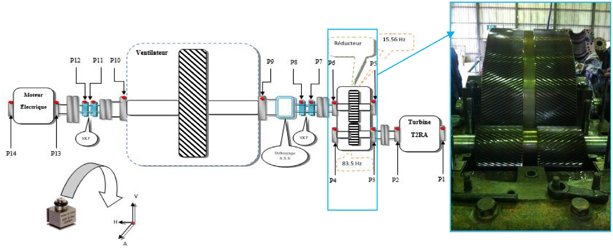
Kinematic diagram of turbo fan 101 BJT, speed reducer GVAB 420.

Measurement acquisition and campaigns carried out

Vibration measurements were taken on the plain bearings (P3 to P6) of the turbofan in three directions. Two types of accelerometers were employed: a triaxial accelerometer (type 4524B-001) and an industrial accelerometer (type 4511-001), as shown in Figure 15(a). To collect and process these measurements, a Brüel & Kjaer PULSE 16.1 analyzer equipped with PULSE LABSHOP acquisition software was utilized, as depicted in Figure 15(b).

Figure 15.

(a) Location of accelerometers and (b) pulse analyzer 16.1.

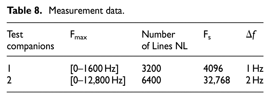
Given the critical role of the 101 BJT turbofan in the cooling process, continuous monitoring is essential. The study was conducted at the national fertilizer production company, where it was observed that this system was primarily monitored offline, relying on overall RMS velocity vibration levels. As these levels were found to be considerably high, test campaigns were initiated across various frequency bands to diagnose the potential causes of this elevated vibration. Table 8 summarizes the key data obtained from these measurements. The objective of these signal measurements was to detect possible impacts within the mechanism, such as those resulting from bearings, gears, blade wear, and more. The frequency bands used by the maintenance department for monitoring the system were inadequate for identifying the aforementioned faults, as they typically occurred at higher frequencies, except in the cases of shaft friction and plain bearing wear.⁴⁵

Table 8.

Measurement data.

Test companions	F_max	Number of Lines NL	F_s	Δf
1	[0–1600 Hz]	3200	4096	1 Hz
2	[0–12,800 Hz]	6400	32,768	2 Hz

Analysis of turbofan 101 BJT and scalar indicators

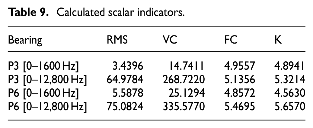
The table below provides scalar indicators computed for bearings 3 and 6 in the turbofan 101 BJR gearbox (see Table 9). These indicators serve to evaluate the presence of faults in each bearing. Upon analyzing these indicators, the following conclusions can be drawn:

➢ For bearing 3 in the high-frequency range [0–12,800 Hz], the value of K exceeds 3, indicating the presence of faults in this bearing. Additionally, the RMS and CF values are substantial, further supporting the indication of defects.

➢ For bearing 6 in the low-frequency range [0–1600 Hz], the value of K surpasses 3, suggesting the presence of an anomaly in this bearing. Furthermore, in the high-frequency range, the RMS, VP, and K values all align to indicate the presence of a fault in bearing 6.

Table 9.

Calculated scalar indicators.

Bearing	RMS	VC	FC	K
P3 [0–1600 Hz]	3.4396	14.7411	4.9557	4.8941
P3 [0–12,800 Hz]	64.9784	268.7220	5.1356	5.3214
P6 [0–1600 Hz]	5.5878	25.1294	4.8572	4.5630
P6 [0–12,800 Hz]	75.0824	335.5770	5.4695	5.6570

Application of cyclostationarity to signals measured on gearbox bearings and cyclostationary indicators

The table below displays cyclic indicators computed for stages 3 and 6 of the turbofan 101 BJR gearbox (see Table 10). From the analysis of these indicators, the following conclusions can be drawn:

For stage 3, both the psychoacoustic roughness and cyclic roughness values increase as the frequency range expands, rising from 1.53 to 1.71 Hz and from 1.43 to 2.22 Hz, respectively. This suggests that these two indicators become more reliable at higher frequencies.

Similarly, for stage 6, the psychoacoustic roughness and cyclic roughness values also exhibit an increase as the frequency range extends, with values going from 1.73 to 1.81 Hz and from 1.98 to 2.52 Hz, respectively. This indicates that these indicators gain greater reliability at higher frequencies as well.

Table 10.

Calculated cyclostationarity indicators.

Bearing	Psychoacoustic roughness	Cyclic roughness
P3 [0–1600 Hz]	1.530	1.434
P3 [0–12,800 Hz]	1.709	2.224
P6 [0–1600 Hz]	1.730	1.975
P6 [0–12,800 Hz]	1.809	2.524

Low-frequency analysis of the gear Reducer

A. Input bearing

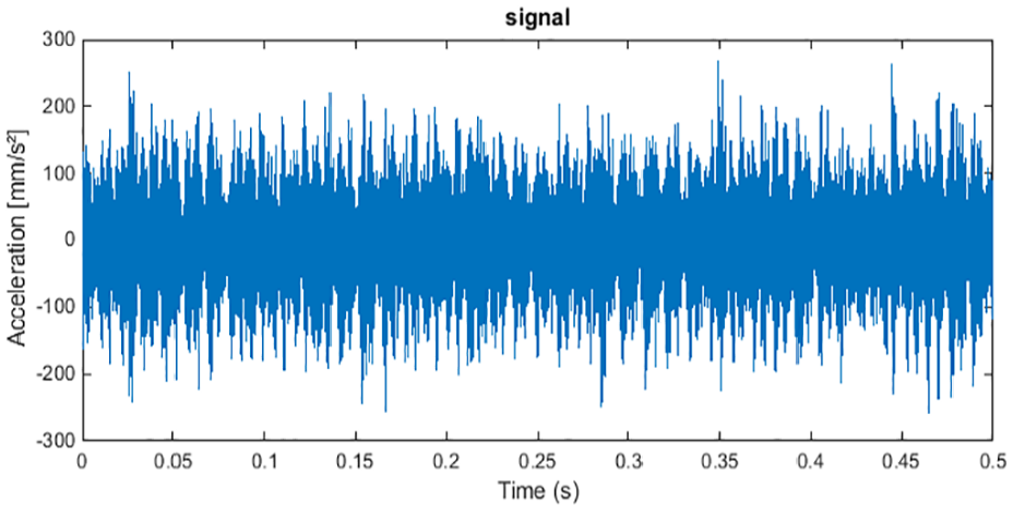
The application of the DIM on the signal from stage 3 of the gearbox (see Figure 16), measured in the frequency band [0–1600 Hz] and illustrated in Figure 17(a), reveals the appearance of two cyclic frequencies: the first, α₂ = 3.798 × 10⁻³*f_s ≈ 15.56 Hz (with f_s = 4096 Hz), corresponds to the rotation frequency of the pinion. The second cyclic frequency, α₁ = 0.02*f_s≈ 83.5 Hz, presents a significant amplitude and corresponds to the rotation frequency of the wheel. The modulations of these two cyclic frequencies indicate generalized wear on the teeth of both wheels.

Figure 16.

Acceleration signal measured on stage 3 in the band [0–1600 Hz].

Figure 17.

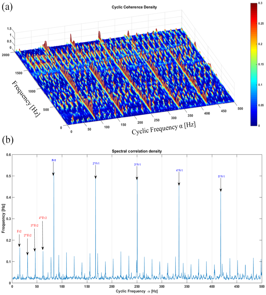
(a) Spectral correlation (DIM), (b) its integration (IDIM) of the signal in Figure 16.

The application of IDIM makes it possible to clearly and visibly highlight these two cyclic frequencies and their modulations, as shown in Figure 17(b).

B. Output bearing

The application of DIM to the signal from stage 6 of the gearbox (see Figure 18), measured in the frequency range [0–1600 Hz] and illustrated in Figure 19(a), reveals the presence of two cyclic frequencies. The first, α₂= 3.798 × 10⁻³*f_s ≈ 15.56 Hz (with f_s = 4096 Hz), corresponds to the rotation frequency of the pinion, while the second, α₁= 0.02 *f_s ≈ 83.5 Hz, has significant amplitude and corresponds to the rotation frequency of the wheel. The modulations of these two cyclic frequencies indicate generalized wear on the teeth of both wheels.

Figure 18.

Acceleration signal measured on stage 6 in the band [0–1600 Hz].

Figure 19.

(a) Spectral correlation (DIM), (b) its integration (IDIM) of the signal in Figure 18.

The application of IDIM further enhances the visibility of these two cyclic frequencies and their modulations, as depicted in Figure 19(b).

High-frequency analysis of the reducer

A. Input bearing

The application of DIM to the signal from stage 3 of the gearbox (see Figure 20), measured in the frequency range [0–12,800 Hz] and illustrated in Figure 21(a), reveals the presence of two cyclic frequencies. The first, α₂ = 1.83 × 10⁻⁴ Hz * f_s ≈ 6 Hz (with f_s = 32,768 Hz), corresponds to 0.38 × Fr₂, indicating the presence of an oil swirl defect in the pinion. Additionally, there is a carrier frequency at 1044 Hz and its harmonics (2088, 3132, and 4176 Hz), which may correspond to frequencies generated by the turbine. Furthermore, there is a significant peak corresponding to the second harmonic of the wheel rotation frequency (Fr₁), suggesting a misalignment fault.

Figure 20.

Acceleration signal measured on stage 3 in the band [0–12800 Hz].

Figure 21.

(a) Spectral correlation (DIM), (b) its integration (IDIM) of the signal in Figure 20.

The application of IDIM enhances the visibility of the cyclic frequency and its modulations, and reveals a peak corresponding to 0.5 × Fr₁, indicating an oil swirl fault on the reducer wheel, as shown in Figure 21(b).

B. Output bearing

The application of DIM to the signal from stage 6 of the gearbox, measured in the frequency range [0–12,800 Hz] and illustrated in Figure 22, reveals the presence of the cyclic frequency α₂ = 4.74 × 10⁻⁴*f_s ≈ 15.56 Hz (with f_s = 32768 Hz), corresponding to the rotation frequency of the wheel (Fr₂) and its harmonics. The modulations of this cyclic frequency clearly indicate the generalized wear of the pinion teeth. Additionally, there is a carrier frequency at 2088 Hz, corresponding to the second harmonic of the turbine fault frequency, along with its fourth and sixth harmonics (4055 and 6122 Hz), as illustrated in Figure 23(a). The application of IDIM enhances the visibility of the cyclic frequency and its modulations, as shown in Figure 23(b).

➢ Observation for Analysis

Figure 22.

Acceleration signal measured on stage 6 in the band [0–12800 Hz].

Figure 23.

(a) Spectral correlation (DIM), (b) its integration (IDIM) of the signal in Figure 22.

In conclusion, the results obtained from applying cyclostationarity analysis based on DIM and IDIM convincingly demonstrate the effectiveness of this method in detecting gear faults. This approach proves superior to spectral, cepstral, and envelope analysis, especially in the presence of noise, exhibiting enhanced detection capabilities as the noise level increases.

The simulation study highlights the inadequacy of scalar indicators K and FC in effectively detecting characteristic signal changes under significant noise conditions. Conversely, cyclic roughness and psychoacoustic roughness indicators prove more effective in identifying anomalies, offering more accurate detection.

✓ Our simulation and in-depth study have enabled us to establish intervals for cyclostationary indicators used as thresholds for gear fault detection. The observed values of psychoacoustic roughness and cyclic roughness indicators during the simulation range between 0.18 and 1.39 Hz, and between 0.18 and 1.62 Hz, respectively, clearly indicating the presence of faults in the gearing system. Furthermore, the calculation of these indicators on real signals from the gearbox reveals additional ranges for psychoacoustic roughness between 1.53 and 1.81 Hz, and cyclic roughness between 1.43 and 2.52 Hz, definitively indicating anomalies in the system.

✓ This analysis clearly demonstrates the superiority of cyclostationary analysis and its indicators compared to classical analyses such as spectral and cepstral analysis, as well as scalar indicators. These results reinforce the effectiveness of this method in the accurate detection of gear faults, even in the presence of noise.

Conclusion

This paper constitutes a substantial contribution to the domain of vibration analysis in rotating machines and condition-based preventive maintenance. It highlights the superior efficiency of the cyclostationary method when compared to other vibration analysis techniques, thereby paving the way for enhanced accuracy and reliability in defect detection and severity assessment.

➢ The conducted research delved into diagnostic enhancement through the analysis of both simulated signals and raw time signals measured on the gearbox bearings in the radial direction. Various techniques were employed, including fast Fourier transform (FFT) for signal spectrum, band-pass filtering utilizing a butterworth filter, envelope analysis to extract defect features, and the integration of cyclostationary analysis with the Hilbert transform for enhanced fault detection. These advancements present promising avenues for elevating condition-based preventive maintenance and ensuring the heightened reliability of rotating machines.

➢ This research establishes a digital simulation model for double faults, providing a robust tool for generating essential signals to optimize threshold determinations for defect detection indicators. Moreover, it aids in comprehending the vibration dynamics of geared power transmission systems. The simulated signals accurately replicate double faults, allowing for a detailed exploration of their impact on the system’s vibration characteristics. Consequently, these signals serve as a valuable resource for advancing defect detection techniques. They facilitate the precise definition of detection thresholds and the study of specific vibration behaviors associated with various combined defects. The findings of this study illuminate the significance of this approach in improving gear fault detection and analysis.

➢ Classical and cyclostationary scalar indicators, such as kurtosis, crest factor, psychoacoustic roughness, and cyclic roughness, have traditionally proven effective in detecting shock-type defects due to their sensitivity to periodic pulses. However, these indicators face limitations in the presence of combined faults, largely attributed to operational noise and parasitic components.

➢ This study delves into the application of cyclostationary analysis, coupled with the Hilbert transform, unveiling promising outcomes. This innovative approach boasts several advantages, such as representing signal distribution intensity modulation (DIM), employing a cascade decomposition technique to segregate higher and lower-frequency components, and utilizing both conventional scalar and cyclostationary indicators for detecting shock-type faults. The research demonstrates the potential for enhanced machinery fault detection through the amalgamation of classical and cyclostationary analysis with advanced signal processing techniques.

➢ This research makes a substantial contribution by enhancing our understanding and providing more precise diagnoses of defects in rotating machines. Through the application of advanced vibration analysis techniques, these findings play a crucial role in improving the effectiveness of condition-based preventive maintenance. Ultimately, this contributes to prolonging the operational life of machinery and reducing operating costs in the rotating machinery sector.

Footnotes

Appendix

Notation

Abbreviations	Designation
$R_{x}^{α} (α)$	Cyclic autocorrelation function
${SC}_{x}^{α} (f)$	Spectral correlation density
${DIM}_{Δ f}^{PSC} (f, α)$	Distribution intensity modulation function
$D I M_{Δ f}^{P S C o h} (f, α)$	Spectral coherence distribution intensity modulation
$x_{Δ f} (t, f)$	Filtered signal in a side frequency band $[f - \frac{Δ f}{2}; f + \frac{Δ f}{2}]$
f	Carrier frequency
F_m	Meshing frequency
Fs	Sampling frequency
V_C	Peak value
Fr₁	Reducer input shaft rotation frequency
Fr₂	Reducer output shaft rotation frequency
F₁, F₂	The lower and upper limits of the domain of integration
f_s	Sampling frequency
I	The number of summed frequencies
$γ_{x}^{2} (α_{l}, f_{k})$	Fast Estimator of Order-Frequency Spectral Coherence
F _C	Crest Factor
N _e	Number of spectrum lines
F _max	Maximum frequency
x_Δf (t,f)	Indicates the filtered version
Δf	The step frequency
A _i, B_i	Amplitudes
RMS	Root Mean Square
K	Kurtosis
DSC ^α	Spectral correlation
N _p	Nombre the blades
NL	Number of Lines

Acknowledgements

The authors would also like to thank the company’s maintenance crew for their assistance.

Handling Editor: Qibin Wang

Author contributions

Kebabsa Tarek: Conceptualization, Investigation, Methodology, Supervision, Writing– review & editing.

Babouri Mohamed Khemissi: Conceptualization, Methodology, Investigation, Writing – review & editing.

Abderrazek Djebala: Investigation, Writing – review & editing.

Ouelaa Nouredine: Investigation, Methodology, Writing – review & editing.

Declaration of conflicting interests

The author(s) declared no potential conflicts of interest with respect to the research, authorship, and/or publication of this article.

Funding

The author(s) disclosed receipt of the following financial support for the research, authorship, and/or publication of this article: This work was carried out with the material resources of the Laboratory of Mechanics and Structures, University of 08 May 1945 Guelma, with the support of the Algerian ministry of higher education and scientific research, the delegated ministry for scientific research (via PRFU project code: A14N01EP230220220002.

Ethics approval

The work contains no libellous or unlawful statements, does not infringe on the rights of others, or contains material or instructions that might cause harm or injury.

Consent to participate

The authors consent to participate.

Consent for publication

The authors consent to publish.

Code availability

Not applicable

Ethical statement and disclosure of potential conflict of interest for the paper entitled

Case Study: Condition-Based Maintenance Using Cyclostationary Analysis and Numerical Modeling with Innovative Indicators.

ORCID iD

Tarek Kebabsa

References

Lejeune

Lacoume

Marchand

, et al. Cyclostationarities of order 1 and 2: application to vibration signals of gears. In: 16thGRETSI conference on Signal and Image Processing, GRETSI, 1997.

Kidar

Thomas

Badaoui

, et al. Diagnosis of gear faults by cyclostationarity. Chartres, France: Institute of Technology, 2013.

Kebabsa

Ouelaa

Antoni

, et al. Experimental study of a turbo-alternator in industrial environment using cyclostationarity analysis. Int J Adv Manuf Technol 2015; 81: 537–552.

Feng

Wang

, et al. A case study of sample entropy analysis to the fault detection of bearing in wind turbine. Case Stud Eng Fail Anal 2017; 9: 99–111.

Gao

Liu

Tang

, et al. A novel wind turbine fault diagnosis method based on intergral extension load mean decomposition multiscale entropy and least squares support vector machine. Renew Energy 2018; 116: 169–175.

Kebabsa

Babouri

Djebala

, et al. Advanced diagnostic techniques for turbo compressors: a spectral analysis approach for preventive maintenance. Adv Mech Eng 2024; 16: 1–21.

Lei

Liu

Jiang

Fault diagnosis of wind turbine based on long short-term memory networks. Energy 2019; 133: 422–432.

Feng

Liang

, et al. A fault diagnosis method for planetary gearboxes under non-stationary working conditions using improved Vold-Kalman filter and multi-scale sample entropy. J Sound Vib 2019; 439: 271–286.

Kumar

Gandhi

Zhou

, et al. Latest developments in gear defect diagnosis and prognosis: a review. Measurement 2020; 158: 107735.

10.

Feng

Smith

Borghesani

, et al. Use of cyclostationary properties of vibration signals to identify gear wear mechanisms and track wear evolution. J Signal Process Syst 2021; 150: 107258.

11.

Kumar

Parey

Kankar

PK.

Vibration based fault detection of polymer gear. Mater Today Proc 2021; 44: 2116–2120.

12.

Feng

Wang

, et al. A novel order spectrum-based Vold-Kalman filter bandwidth selection scheme for fault diagnosis of gearbox in offshore wind turbines. Ocean Eng 2022; 266: 112920.

13.

Feng

, et al. A novel cyclic-correntropy based indicator for gear wear monitoring. Tribol Int 2022; 171: 107528.

14.

Feng

A novel gear fatigue monitoring indicator and its application to remaining useful life prediction for spur gear in intelligent manufacturing systems. Int J Fatigue 2023; 168: 107459.

15.

Feng

, et al. A review of vibration-based gear wear monitoring and prediction techniques. Mech Syst Signal Process 2023; 182: 109605.

16.

Heng

RBW

Nor

MJM

. Statistical analysis of sound and vibration signals for monitoring rolling element bearing condition. Appl Acoust 1998; 53: 211–226.

17.

Belsak

Flasker

Detecting cracks in the tooth root of gears. Eng Fail Anal 2007; 14: 1466–1475.

18.

Cousinard

Marconnet

. Detection of gear damage using cepstral analysis and envelope detection: Industrial application and validation for the diagnosis of a gearbox operating at low speed. In: 16th French Mechanics Congress Nice, 1–5 September 2003.

19.

Chaari

Fakhfakh

Haddar

Numerical simulation of the dynamic behavior of a gear transmission in the presence of tooth defects. Mec Ind 2006; 6: 625–623.

20.

Pachaud

Salvetat

Fray

Crest factor and kurtosis contributions to identify defects inducing periodical impulsive forces. Mech Syst Signal Process 1997; 11: 903–916.

21.

Benchaabane

Optimization of fault identification parameters in gear transmissions by vibration analysis. Master’s Thesis, University of Guelma, 2008.

22.

Benchaabane

Djebala

Ouelaa

, et al. Vibration diagnosis of gear faults based on scalar indicators. In: Algerian mechanical congress CAM, Biskra, November 2009.

23.

Djebala

Ouelaa

Hamzaoui

, et al. Optimization of the use of scalar indicators in the context of predictive maintenance of rolling bearings. In: Algerian congress of construction mechanics, April 2007.

24.

Capdessus

Sidahmed

Applications. Analysis of the vibrations of a gear: cepstrum, correlation, spectrum. Signal Process 1992; 8: 365–372.

25.

Djebala

Ouelaa

Benchaabane

, et al. Application of the wavelet multi-resolution analysis and Hilbert transform for the prediction of gear tooth defects. Meccanica 2012; 47: 1601–1612.

26.

Boulenger

Conditional maintenance by vibration analysis, maintenance treaty. Engineering Techniques MT 9285, version, 2005.

27.

Urbanek

Barszcz

Antoni

Time–frequency approach to extraction of selected second-order cyclostationary vibration components for varying operational conditions. Measurement 2013; 46: 1454–1463.

28.

Urbanek

Barszcz

Antoni

. A two-step procedure for estimation of instantaneous rotational speed with large fluctuations. Mech Syst Signal Process 2013; 38: 96–102.

29.

Urbanek

Barszcz

Antoni

Integrated modulation intensity distribution as a practical tool for condition monitoring. J Appl Acoust 2014; 77: 184–194.

30.

Antoni

Randall

RB.

The spectral kurtosis: application to the vibratory surveillance and diagnostics of rotating machines. Mech Syst Signal Process 2006; 20: 308–331.

31.

Antoni

Cyclic spectral analysis in practice. Mech Syst Signal Process 2007; 21: 597–630.

32.

Antoni

Cyclic spectral analysis of rolling-element bearing signals: facts and fictions. J Sound Vib 2007; 304: 497–529.

33.

Antoni

Blind separation of vibration components. Principles and demonstrations. Mech Syst Signal Process 2005; 19: 1166–1180.

34.

Kebabsa

. Study of aspects of failures and conditional preventive maintenance techniques applied to turbomachine. Doctoral Thesis defended, Badji Mokhtar Annaba University, Faculty of Engineering Sciences, 2016, https://biblio.univ-annaba.dz/?page_id=2452 (accessed May 2016).

35.

de Pater

Mitici

. Predictive maintenance for multi-component systems of repairables with remaining-useful-life prognostics and a limited stock of spare components. Reliab Eng Syst Saf 2021; 214: 107761.

36.

Bevilacqua

Braglia

The analytic hierarchy process applied to maintenance strategy selection. Reliab Eng Syst Saf 2021; 70: 71–83.

37.

Borghesani

Randall

, et al. Removal of transfer function effects from gear vibration signals under constant and variable speed conditions. Mech Syst Signal Process 2023; 184: 109714.

38.

Kumar

Goyal

Dang

, et al. Condition monitoring parameters for fault diagnosis of fixed axis gearbox: a review. Mater Today Proc 2018; 5: 6128–6137.

39.

Tchakoua

Wamkeue

Ouhrouche

, et al. Wind turbine condition monitoring: state-of-the-art review, new trends, and future challenges. Energies 2014; 7: 2595–2630.

40.

Zhao

Wang

, et al. Hierarchical hyper-Laplacian prior for weak fault feature enhancement. ISA Trans 2020; 96: 429–443.

41.

Nentwich

Reinhart

A method for health indicator evaluation for condition monitoring of industrial robot gears. Robotics 2021; 10: 80.

42.

Moumene

Identification of mixed gear and bearing defects by vibration analysis. Doctoral Thesis, Badji Mokhtar Annaba University, Faculty of Engineering Sciences, 2010.

43.

Kass

Autonomous vibratory diagnosis of bearings. Vibrations [physics.class-ph]. University of Lyon; Lebanese University. French. <NNT: LYSEI103>. https://theses.hal.science/INSA-LYON-THESES/tel-02902122v1 (2019, accessed August 2024).

44.

Kass

Raad

Antoni

. Self-running bearing diagnosis based on scalar indicator using fast order frequency spectral coherence. Measurement 2019; 138: 467–484.

45.

FERTIAL Maintenance Department. 101 BJT turbofan unit. Technical document (Date not specified).

Case study: Condition-based maintenance using cyclostationary analysis and numerical modeling with innovative indicators

Abstract

Keywords

Introduction

Sampling and scanning techniques

Gaussian white noise

Numerical modeling and simulation of double gear defects and scalar indicator calculation

Study of the influence of fault amplitudes on scalar indicators and vibration signature

A. Study of the influence of fault amplitudes on scalar indicators

B. Study of the influence of fault amplitudes on the vibration signature

Study of the influence of rotation frequencies on scalar indicators and vibration signature

A. Study of the influence of rotation frequencies on scalar indicators

B. Study of the influence of rotation frequencies on the vibration signature

Study of the influence of meshing frequencies on scalar indicators and vibration signature

A. Study of the influence of meshing frequencies on scalar indicators

B. Study of the influence of meshing frequencies on the vibration signature

Cyclostationarity analysis: Theory, indicators, and applications

Cyclostationary indicators

Application of cyclostationary analysis to simulated signals

A. Case 1: Fault amplitudes and varying fault amplitudes with noise

B. Case 2: Rotational frequencies and varying rotational frequencies with noise

C. Case 3: Varying meshing frequencies with and without noise

Experimental study

Description of the installation

Measurement acquisition and campaigns carried out

Analysis of turbofan 101 BJT and scalar indicators

Application of cyclostationarity to signals measured on gearbox bearings and cyclostationary indicators

Low-frequency analysis of the gear Reducer

A. Input bearing

B. Output bearing

High-frequency analysis of the reducer

A. Input bearing

B. Output bearing

Conclusion

Footnotes

Appendix

Acknowledgements

Author contributions

Declaration of conflicting interests

Funding

Ethics approval

Consent to participate

Consent for publication

Code availability

Ethical statement and disclosure of potential conflict of interest for the paper entitled

ORCID iD

References