Sage Journals: Discover world-class research

Abstract

To detect possible failures of the pressure sensor in the fuel cell engine air supply subsystem, this study proposes a fault identification method based on Random forest. To simulate faults in the sensor, we injected deliberate faults and constructed a fault dataset based on it. This dataset includes gradual fixed deviation and gradual complete deviation. The peRandom forestormance of training accuracy is observed on different fault datasets, aiming to identify fault types based on the deviation in accuracy caused by the presence of polluted or corrupted samples in the dataset. The results indicate that machine learning can effectively distinguish the data collected within 9 min. The validity of the residual law established by the root mean square error (RMSE) can be demonstrated through an example, wherein successful identification of intermittent faults 1.2/1.5 can be achieved a difference of 33%, which can effectively distinguish fault categories. In addition, this method does not rely on high-precision models and effectively utilizes abundant sensor data and the uneven distribution of data sets under faults, including sensors other than the target fault sensor, for machine learning to identify different types of sensor faults.

Keywords

Fuel cell sensor random forest fault identification

Introduction

Currently, with the rapid global development of hydrogen production, hydrogen storage, and hydrogen refueling technology, there has been a significant increase in investments by stack-related enterprises and the establishment of industry standards.^1–5 The manufacturing technology for membrane electrode components has become more mature.⁶ The research conducted by manufacturers on the main components of fuel cells is increasingly becoming more comprehensive and refined. So a mature research and development system has been formed.⁷ In the coming decades, hydrogen fuel cell vehicles will undoubtedly emerge as a strategic choice for countries and enterprises. However, due to the characteristics of hydrogen, there are potential safety hazards in the hydrogen-related operation link.⁸ Fuel cell contain multiple subsystems, and it is important to note that most sensors can be influenced by the surrounding environment.^9–11 For instance, the pressure sensor in the air supply subsystem may experience failure due to the condensation of liquid water.

The stable operation of fuel cell vehicles relies heavily on the information provided by a multitude of sensors as a reference.¹² Once the running data is available, the next step of status detection and fault identification can be peRandom forestormed. Common ones are active fault tolerance and passive fault tolerance.¹³ All of them have achieved good results in various fields.^14,15 To ensure the proper functioning of the equipment, Fault Detection and Isolation (FDI) systems are often designed.¹⁶

Jouin et al. proposed a Prediction and Health Management (PHM) framework, with the first layer focused on data acquisition through sensors.¹⁷ It can be seen that if the data acquisition of the first layer fails, subsequent processes such as data processing, scenario assessment, and diagnosis in the following layers will not accurately reflect the real state.^18,19 Therefore, it is of utmost importance to effectively identify sensor failures, as timely diagnosis of sensor faults plays a vital role in ensuring the safety of fuel cell vehicles.²⁰ Yan et al. constructed a thermal model comprising 42 equations and introduced an Active Fault Tolerant Control (AFTC) strategy that substantially enhanced the control peRandom forestormance of the stack. The simulation utilized the Offset Fault and Multiplicative Fault, followed by the successful diagnosis of sensor faults using the residual model.²¹ In practical applications, as the usage of fuel cell increases and working conditions change, it is necessary to further validate the migration and stability of the residual model. Elkhatib Kamal proposed a Takagi-Sugeno (TS) fuzzy model affected by the sensor, defined the state space equation of Proton Exchange Membrane Fuel Cell (PEMFC) using matrices and functions, and utilized the Fuzzy Unknow Input Observer (FUIO) algorithm to effectively reduce the error between sensor prediction estimates and sensor normal values,²² Fuzzy logic control is an intelligent control system that mimics the way of human thinking.^23,24 All of these approaches mentioned above are model-based.

Mao et al. introduced the concept of sensor reliability in their research. They suggested using voltage-sensitive sensors for diagnostics to enhance the accuracy of the diagnosis. It was discovered that removing abnormal sensors led to improved diagnostic results.²⁵ Another study by Zhang et al. proposed an online diagnostic approach specifically for intermittent sensor faults.²⁶ These works illustrate that sensor failure is a critical issue in fuel cell. The accuracy of data acquisition from various sensors is influenced by the operating state of the fuel cell, resulting in different types of sensor failures.

Wang and Li addressed the issues of complex modeling and poor portability by proposing the use of Spiking Neural Networks (SNN) for sensor fault diagnosis. They also highlighted the limitations of deep learning, such as low robustness, data dependence, and high resource consumption.²⁷ Many challenges in the field of deep learning remain unsolved. Firstly, there is still a considerable gap between academic theory and practical application in online vehicle diagnosis. Secondly, some problems arise when combining algorithm usage with fault diagnosis, including the pursuit of high accuracy at the algorithm level and the integration of new algorithms with traditional fault detection methods. The true power of machine learning algorithms lies in their ability to uncover intrinsic relationships among large amounts of data, which often involves using a black-box model. This intrinsic relationship encompasses multiple metrics beyond the prediction accuracy on a single test set.

Quan et al. utilized the Levenberg-Marquardt (LM) algorithm for constructing an Artificial Neural Network (ANN) model, which was deployed to detect faults in the current sensors of the air supply subsystem.²⁸ Oh et al. used representative residual and machine-learning-based methods to diagnose faults in the air mass flow sensor and thermocouples.^29–31 Gong et al. utilized a sensor pre-selection method to enhance the accuracy of the diagnosis.³² Therefore, the identification of sensor faults not only enhances the stability of closed-loop control of fuel cell but also accelerates the process of sensor pre-selection in fault diagnosis. This, in turn, increases the accuracy of fault diagnosis by eliminating faulty sensors.

There exists a significant correlation between sensor failures and the failures of the corresponding systems.^33,34 Furthermore, there may be interdependencies among different sensor failures, such as step faults, pulse faults, noise faults, stuck faults, drift faults, and periodic faults.^9,35

The fuel cell bench sensor can present the measured data in the form of a data set, which serves as the most direct representation of the sensor’s working results. It is crucial to discover effective troubleshooting methods for sensors designed for in-vehicle applications.³⁶ Data-driven fault diagnosis has been equally successful in other areas, such as the good performance of unsupervised learning methods for Main Steam Line Break (MSLB) faults in nuclear power plants, Collecting failure data in industry can be difficult, expensive, or even impossible, and unsupervised learning offers an effective alternative.³⁷ Ball bearings are sorted according to Fisher features with good accuracy,³⁸ and bearing fault classification based on fault image datasets.³⁹ At the same time, the Random forest adopted in this paper has also achieved certain results in fault classification learning.⁴⁰ This paper primarily utilizes a residual-based Random forest to identify fault datasets by intentionally injecting faults into the sensor. Although there are many types of sensor faults, this paper examines typical fixed, complete, and intermittent deviations

Then, by calculating the RMSE of the subsequent forest training results, we generate the residual between the measured value and the normal value when a specific fault occurs in the sensor. This residual-based approach allows for distinguishing various common types of sensor faults, thereby achieving accurate diagnostic outcomes.

Random forest-based approach

Random forest is a classic machine learning method that uses random sampling with a return on the dataset, as shown in Figure 1. Even though the training set and test set are separated, the division is purely based on the number of datasets. The data allocated to the test set can still be randomly sampled and included in the training set during the machine learning process, and vice versa. Therefore, modifying the output data of the test set will effectively modify the overall dataset. This interference can disrupt the training process by introducing artificially created data that does not align with real operating conditions. Consequently, the final training outcome will reflect the extent to which the dataset has been contaminated by inaccurate samples. This paper is also the first to propose sensor fault identification based on the severity of dataset pollution. By the RMSE of the results to reflect the difference between the predicted and actual values. Different RMSE manifestations for different types of faults can create residuals for identifying sensor faults and distinguishing between different sensor faults. In the past, excessive attention was given to the test set, but this article primarily focuses on analyzing the deviation between the faulty state and the normal state.

Figure 1.

Random forest algorithm construction flowchart.

The Random forest algorithm has a good performance effect on high-dimensional large-sample datasets. A variety of sensor data can theoretically train a black-box model similar to a fuel cell engine. However, the training process can be affected by data pollution caused by sensor failure, leading to deviations in the final trained model from the actual working state of the fuel cell engine. In this paper, the main focus is on evaluating the degree of bias in the training model, rather than solely relying on traditional research criteria such as test set accuracy.

The Random forest uses the autonomous sampling method to train a base learner for each sampled training subset. The regression task uses the averaging method to combine these base learners. In a given dataset D containing m samples, a random sample is selected from it and put into another sampling set D^’ hen the sample is put back into the original dataset D, so that the sample may still be selected in the next sampling. Therefore, after m random sampling operations, we obtain the sampling set D^’ containing m samples. The probability of not being picked at once in a sample is about 36.8% as in equation (1). So the sample that is not selected at all can be used as the test set (36.8%) and the selected sample as the training set (63.2%). However, since the goal of this paper is to reflect the degree of contamination of the entire dataset by using the RMSE results of the training set, the sample size of the training set is expanded to 70% (4140). The test set consisting of fault data injections makes up 30% of the dataset (1774). Due to the randomness of Random forest sampling, the data in the test set will also be extracted into the training set. Because the Out-of-Bag Estimate (OOB) method can only quantitatively divide the train set and the test set without training on the specific specified samples, it provides the possibility for the successful identification of the more hidden intermittent sensor faults in this method.

lim_{m \to \infty} {(1 - \frac{1}{m})}^{m} = \frac{1}{e}

(1)

To eliminate the dimensional influence between the sensor data, the dataset set is normalized to the data in the range of (0,1).

y = \frac{(y_{\max} - y_{\min}) * (x - x_{\min})}{x_{\max} - x_{\min}} + y_{\min}

(2)

y is the normalized value, x is the initial value, x_max is the maximum value in the initial value, x_min is the minimum of the initial value, y_min = 0, y_max = 1. Therefore, the formula can be reduced to equation (3)

y = \frac{x - x_{\min}}{x_{\max} - x_{\min}}

(3)

Set trees = 100 and leaf = 1. The corresponding error curve is shown in Figure 2, which proves that the adjusted parameters are relatively stable.

Figure 2.

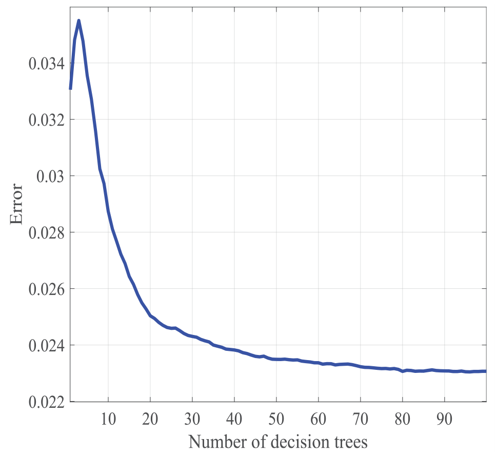
Random forest error curves.

It is assumed that the algorithm contains T basis learners.

{h_{(1)}, h_{(2)}, \cdot \cdot \cdot, h_{(T)}}

(4)

The output of each base learner on sample x is h_i(x). The combination strategy of the average method is used for the numerical output to combine the learning results of each base learner.

In addition, due to the different degrees of influence of the fuel cell subsystem on the air supply subsystem, it is necessary to carry out closed-loop control according to the hydrogen/air supply subsystem sensor data to control the hydrogen-air pressure difference for example. However, the influence of the electrical system on the air supply subsystem is relatively small. The above phenomenon will lead to a large difference in the performance of individual learners. So weighted averaging was used to combine the base learner as follows

H_{(x)} = \frac{1}{T} \sum_{i = 1}^{T} w_{i} h_{i} (x)

(5)

H _(x) is the output prediction value, T is the number of learners, and the weight of the individual learner is h_(i), Usually required w_i≥ 0, $\sum_{i = 1}^{T} w_{i} = 1$ The weights are shown in Figure 3, and the algorithm can assign feature weights to 35 sensor inputs in each training process.

Figure 3.

Random forestfeature weight maps.

The data is then denormalized to output values that match the dimensions of the target fault sensor. The RMSE of the training set is then calculated as shown in equation (6). RMSE is the square root of the square of the deviation from the predicted value to the true value and the ratio of the number of training set M. It measures the deviation between the predicted value and the true value and is sensitive to outliers in the data. The characteristics of RMSE include being intuitive, interpretable, and insensitive to outliers.

RMSE = \sqrt{\frac{1}{M} \sum_{k = 1}^{M} (H_{(x_{k})} - F (x_{k}))}

(6)

M is the total number of samples in the train set (4140), H(x_k) is the output prediction of the kth sample, and F(x_k) is the true value of the output of the k sample.

The identification of sensor faults needs to ensure that there is no voltage drop, which is to ensure the various components of the stack are in normal operation. Since the threshold for normal operation of the sensor is difficult to define, if the voltage sensor has intermittent slow deviation fault while the stack is operating normally. It will hinder the troubleshooting of normal systems.

The basic judgment logic of the sensor is to first look for whether the first feature appears, and continue to use the method of polluting the dataset based on the bad samples of Random forest to diagnose when it does not appear. It is worth noting that the fault of the first feature is the strongly coupled state of the sensor fault and the stack fault, and it is impossible to determine what the cause of the fault is. However, from the perspective of subsequent normal engine monitoring or from the perspective of sensor failure, both faults are fatal: the former loses detection ability, and the latter false fault false alarm. Therefore, the dataset used in this paper is to monitor the normal operation of the fuel cell in the absence of the first feature of voltage drop.

Machine learning process and result analysis

Fault injection to construct a failure data set

The sensor data was obtained from a real uh fuel cell engine, and the experimental setup is shown in Figure 4. The flow chart of the proposed method is shown in Figure 5.

Figure 4.

Detail photograph of the experiment.

Figure 5.

Methodological process framework.

Due to the lack of fault data in the actual operation of fuel cell engine sensors, the purpose of this paper is to inject faults into the sensors to construct a fault data set.

Fault injection 1: slowness changes fixed deviation failure; Fault injection 2: slowness changes complete deviation failure. In this paper, we rely on the fuel cell engine bench in the laboratory of Shandong University of Science and Technology to inject faults into the pressure sensor of the air supply subsystem. The dataset has a total of 5160 data records in 9 min. The dataset includes a total of 36 sensor data types such as current sensor, voltage sensor, compressor temperature sensor, controller temperature sensor, speed sensor, motor current sensor, motor power sensor, motor voltage sensor, etc. Since the air supply subsystem pressure sensor in the actual operation of the fuel cell engine may fail during cold start, the remaining 35 sensor data are selected as input and the air pressure sensor is selected as the output for the dataset. Firstly divide the training set: the test set is 7:3 (3612:1548). Fault injection 1 is then performed: the data in the train set remains unchanged, and only the output data in the test set is injected into the slowness changes fixed deviation failure, which is +0.1, +0.2, +0.3, +0.4 on the basis of the original values, respectively. Finally, fault injection 2 is then performed: the data in the train set remains unchanged, and only the output data in the test set is injected into the slowness changes complete deviation failure, which the values are 1, 1.5, 2.0, 2.5, respectively.

Two faults and different degrees of performance of each fault

A fixed deviation is a fault that adds a fixed value to the normal value to deviate the sensor from the normal state, as shown in Figure 6. Complete deviation is a direct change in the final value of the sensor, as shown in Figure 7. Due to the timing-series nature of the data set, this fault is equivalent to a sudden sensor deviation fault over a certain period of time.

Figure 6.

Different degrees of fixed deviation.

Figure 7.

Different degrees of complete deviation.

Specific operation steps

This paper uses 4° of sensor failure of 2 faults and performs Matlab machine learning 20 times for each fault to eliminate experimental errors. Record the RMSE of the train set results for each machine learning.

Machine learning results and analysis

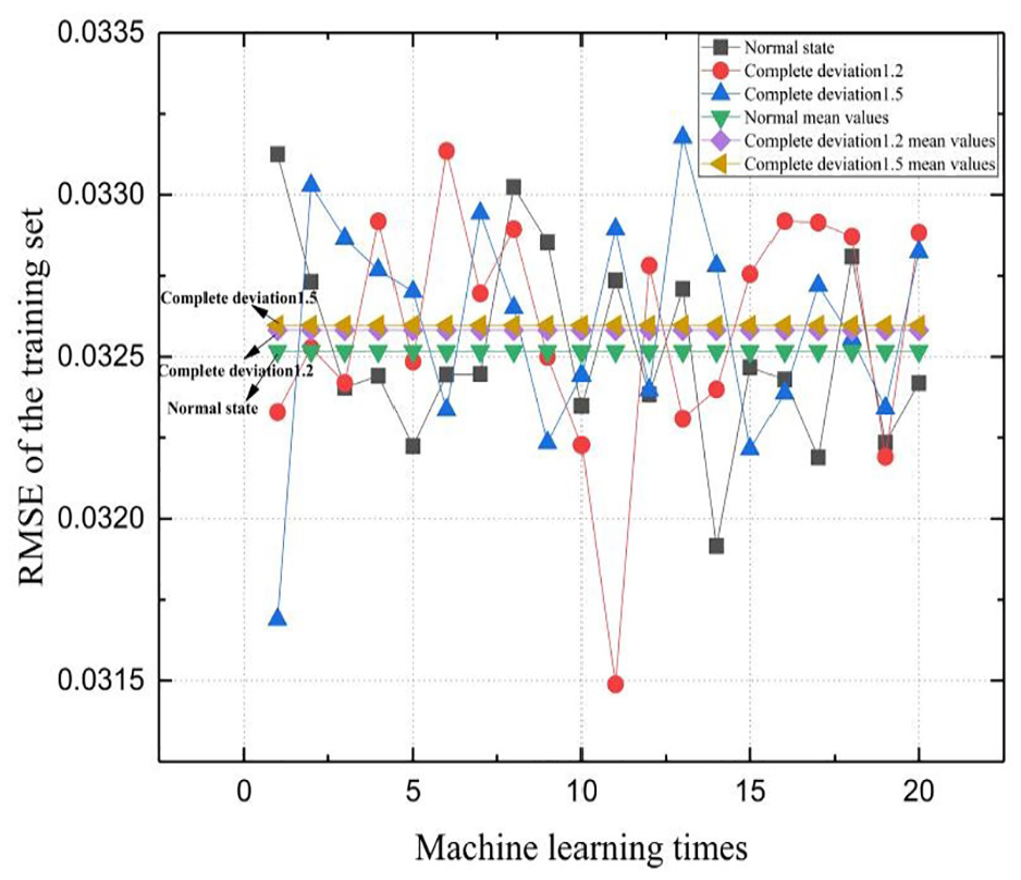
The RMSE after each machine learning under the slow fixed deviation fault is shown in Figure 8, and the fixed deviation will be higher or significantly higher than the normal state at different degrees.

Figure 8.

Fixed deviation with 20 RMSE.

In addition to the fact that the fixed deviation is 0.1, there are many coincidence points with the normal state, and other fixed deviation faults of different degrees will be significantly higher than the normal state. Different degrees of fixed deviation faults can be clearly distinguished. After averaging RMSE, the law is more obvious as shown in Figure 9.

Figure 9.

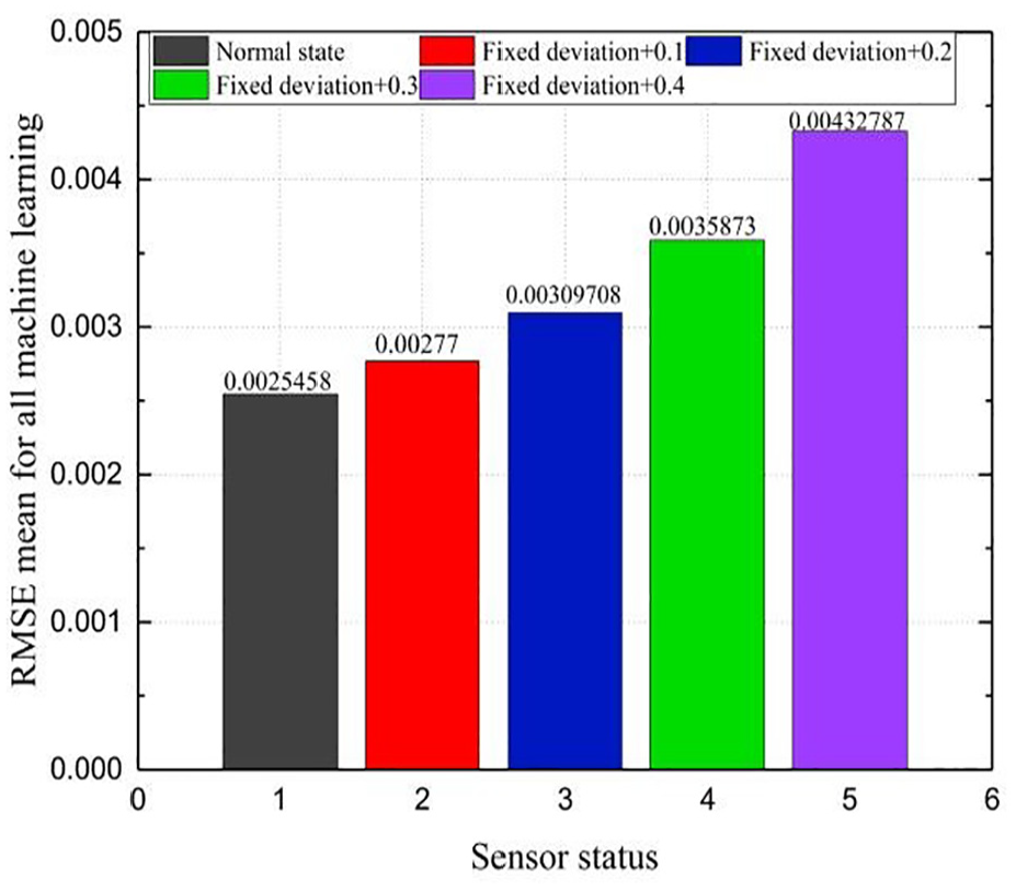
Average of RMSE of fixed deviation.

Explanation of the coincident points in Figure 10: When the test set data is randomly sampled after changing, more normal data from the training set is included. This leads to a reduction in the RMSE of the training model. Conversely, if there is a random sampling of more contaminated data from the test set, it increases the contamination level of the failure data in the entire dataset, resulting in an increase in the RMSE of the trained model.

Figure 10.

Complete deviation with 20 RMSE.

It can be observed that the RMSE sensitivity is higher for different degrees of complete deviation faults compared to fixed deviation faults. The average RMSE values of 20 iterations are depicted in Figure 11 revealing a clear differentiation between different fault degrees.

Figure 11.

Average of RMSE of complete deviation.

According to the average of RMSE, different degrees of faults can be distinguished and fault types can be diagnosed. The reason why the degree of differentiation of a complete deviation fault is higher than that of a fixed deviation is due to varying levels of contamination after data transformation. A complete deviation fault with a progression of 0.5 exhibits greater pollution severity compared to a fixed deviation fault with an increasing deviation of 0.1.

Determination of fault residuals

Firstly, the average RMSE of the machine learning results is calculated for both the fault state and the normal state. This difference is presented in Table 1 as the residual value for gradual fixed deviation in the fault state and normal state. Determining the residuals of different faults provides a reliable method for identifying sensor faults during the actual operation of fuel cell. Therefore, this paper proposes the following method: collect 9 min of data and conduct 20 machine learning cycles. Record the RMSE for each training set and calculate the average. The difference between the RMSE in the unknown state and the normal state is then assessed, and the residuals are calculated accordingly. Finally, the obtained residuals are compared with the residual law mentioned above. By identifying these residuals, the objective of detecting fixed deviation faults and assessing fault severity can be achieved.

Table 1.

Fixed deviation fault residuals.

Sensor status	Fault residuals
Normal state	0
Fixed deviation + 0.1	0.00022573
Fixed deviation + 0.2	0.00055128
Fixed deviation + 0.3	0.00104150
Fixed deviation + 0.4	0.00178207

The residuals for calculating the complete deviation fault are displayed in Table 2. It is evident that the residual values for different degrees of complete deviation faults exhibit good discrimination. Moreover, there is still a certain level of discrimination between the residual values of complete deviation faults and fixed deviation faults. The underlying reason for the variation in residuals among different faults lies in the fact that different sensor values contaminate distinct datasets. Indeed, both random deviation and systematic deviation have distinct impacts on the process of training machine learning models. This can be attributed to the high sensitivity of machine learning algorithms to variations in data extraction and model construction. In terms of residual changes, it is important to note that as the contaminated data deviates further from the true values, the RMSE value of the training set tends to increase. But the closer the polluted data is to the actual value (this situation is also a failure), the smaller the RMSE value of the train set. The incorporation of residuals enhances the efficiency of fault identification. In this study, the fundamental logical sequence for diagnostics is: data extraction, machine learning iterations conducted 20 times, computation of the RMSE for the training set, averaging the RMSE values, and subsequent calculation of residuals. These calculated residuals are then compared against pre-designed fault injections to determine the specific type of fault. The specific residuals corresponding to all faults in this paper are illustrated in Figure 12, providing evidence of the effectiveness of the proposed method.

Table 2.

Complete deviation fault residuals.

Sensor status	Fault residuals
Normal state	0
Complete deviation1.0	0.01008880
Complete deviation1.5	0.00582790
Complete deviation2.0	0.00245824
Complete deviation2.5	−0.00092267

Figure 12.

Summary of fault residuals.

Instance verification

After determining the basic fault residuals and fault identification methods, this paper tests the effectiveness of the method through examples.

The first example involves injecting sensor failure in the same backpressure for a certain period of time, resulting in a complete deviation of 1.2. After performing the same machine-learning steps, the results are shown in Figure 13.

Figure 13.

The RMSE at a complete deviation of 1.2.

It can be found that the RMSE mean value is 0.0107421, the residual difference with the normal value is 0.00820141, and between 0.010088800 and 0.00582790 is consistent with the residual distribution law between the complete deviation 1.0 and the complete deviation 1.5 in the previously determined residual table. It is inferred that the residual law under the back pressure is established and a sensor fault with a complete deviation 1.2 is successfully identified according to the residual.

The sensor fault injection is depicted in Figure 14, with all time periods exhibiting normal values except for the indicated deviations of 1.2 and 1.5. Diagnosing this fault based on threshold setting proves challenging due to the sporadic occurrence of the fault and its deviation value coinciding with the normal state value of some other time period. The machine-learning outcomes presented in Figure 15 provide additional insights.

Figure 14.

Two types of intermittent complete deviation fault.

Figure 15.

RMSE for varying degrees of intermittent complete deviation.

The second example is an intermittent fault, which is difficult to identify in line with the real scenario. This can be observed in Table 3. As can be observed from Table 4, the mean values of RMSE during the intermittent fault state exhibit a significant increase compared to the normal state. This indicates that the presence of faulty data in the dataset adversely affects the modeling accuracy of the final training set.

Table 3.

Time of occurrence of intermittent fault.

Fault injection moment (ms)
10–20	60–70	120–140
340–350	500–510	600–610
650–700	740–770	860–870
990–1000	1050–1060	1100–1110
1260–1270	1290–1390	1440–1445
1500–1505	1597–1599	1623–1626
1688–1690	1726–1729	1861–1872
1922–1931	2000–2350	3300–3650
623–4973	5500–5884	-

Table 4.

Intermittent fault residual values.

Sensor status	Residuals
Normal state	0
Intermittent complete deviation 1.2	6.535E-05
Intermittent complete deviation 1.5	8.075E-05

Moreover, under the influence of this back pressure, a similar residual pattern can still be identified, as shown in Table 4. Fault 1.2 and fault 1.5 can achieve a difference of 33%, which can effectively distinguish fault categories.

Additionally, the greater the deviation from the normal value, the higher the corresponding residual value. Based on these findings, the paper proposes utilizing the existing methods for residual determination and fault identification.

In short, the residual law discovered by RMSE reflects the challenges encountered when inputting normal sensor values and outputting faulty sensor values while establishing data models. Theoretically, this law can be used to identify various sensor states.

At the same time, this paper uses 10-fold cross-validation, divides 10% of the original dataset into the validation set, and compares it with other algorithms, in Figure 16, as shown in the Table 5, Residuals is the difference between the fault state of 1.5 and the normal state, and the results of tree learning can be obtained from the table compared with others. Moreover, RMSE’s Residuals are more distinguishable than other indicators, and they still do not change by orders of magnitude under faults. As can be seen from the figure, the tree still maintains good accuracy in the fault state.

Figure 16.

Algorithm comparison: (a) linear regression, (b) tree and (c) Gaussian SVM.

Table 5.

Comparison of different indicators.

Residuals	RMSE	MSE	R2	MAE
Linear regression	8.116E-2	6.866E-3	0.4482	6.1739E-2
Tree	9.542E-3	1.371E-4	8.98E-3	1.159E-3
Gaussian SVM	5.075E-2	5.180E-3	0.3131	2.638E-2

As shown in Table 6, the proposed method can achieve a 33% difference rate between different fault degrees of intermittent faults that are difficult to identify, indicating that it has better discrimination than traditional methods.

Table 6.

Comparison of results.

Model	Rate of discrepancy
ANN²⁸	9%
UKF⁴¹	2%
RF	33%

The selected pressure sensor is prone to condensate to interfere with the pressure sensor value during the low-temperature cold start, and the selection standard is determined by the power of the fuel cell engine. Under steady-state operating conditions, the pressure sensor should maintain accuracy and stability to ensure that the pressure of the air supply system is effectively monitored, so as to ensure the safe and efficient operation of the system. Under drastic load changes, the sensor fault signal can affect the transient behavior of the system, and the net power of the faulty system can be about 0.2 kW lower than that of the non-faulty system.⁴²

Conclusion

In this paper, a Random Forest-based method for sensor fault identification was proposed. Firstly, faults were injected into the sensor, and a fault dataset was constructed based on the induced faults, specifically focusing on gradual fixed deviation and gradual complete deviation. To address the issue of dataset contamination and its interference with the accuracy of the training model, this paper investigated the performance results under such interference to identify sensor failures. The mean values of the RMSE in the training set were used to determine the residuals between the fault states and normal states. The results demonstrated that this diagnostic method is independent of the accuracy of the algorithm’s test set and the trained model. Only errors in the basic training model needed to be considered, and failure types could be identified by comparing unknown states with normal states. This method was universally applicable to various sensors. Compared with the traditional method, this method can still ensure a certain prediction accuracy with other non-faulty sensors when the target sensor fails, and at the same time, the Random forest is used to capture the characteristics of uneven distribution and abnormal data distribution in the data set, which is better helpful to identify sensor faults, The proposed method can diagnose the sensor data of the actual fuel cell engine within 9 min in about 12 s.

The dataset used in this paper was derived from monitoring data during the operation of a fuel cell engine with no voltage drop characteristics. This method can also identify faults in various sensors by simply finding the residual between the normal state and the unknown state. In other words, if you need to diagnose a sensor fault, you only need to set this sensor as the output value of the Random forestmodel and set other sensors as input values. By fully utilizing the information from each sensor of the fuel cell and training the machine, a black box model can be obtained. This article utilizes machine learning in Matlab, and the Matlab code is 3 KB, making it highly suitable for in-vehicle diagnostic scenarios.

In the future, the research direction should be combined with the cloud data platform to realize the fault diagnosis of multi-sensor system driven by big data, and the method should be extended to other multi-sensor systems.

Footnotes

Handling Editor: Simona Merola

Declaration of conflicting interests

The author(s) declared no potential conflicts of interest with respect to the research, authorship, and/or publication of this article.

Funding

The author(s) disclosed receipt of the following financial support for the research, authorship, and/or publication of this article: 1. Qingdao postdoctoral support project (QDBSH20220202020), 2. Qingdao Natural Science Foundation (23-2-1-110-zyyd-jch), 3. National Natural Science Foundation of China under grants (62203279), 4. Shandong Natural Science Foundation (ZR2023QF073, ZR2023QE208).

ORCID iDs

Yu Haoyi

Wang Zhangu

References

Smitkova

Janicek

Martins

. Hydrogen economy: brief sumarization of hydrogen economy. In: 2022 International conference on electrical, computer and energy technologies (ICECET), Prague, Czech Republic, 2022, pp.1–5.

Weiming

Jiekang

Jinjian

, et al. Capacity allocation optimization framework for hydrogen integrated energy system considering hydrogen trading and long-term hydrogen storage. IEEE Access 2023; 11: 15772–15787.

Zhang

Chen

, et al. Planning of hydrogen refueling stations in urban setting while considering hydrogen redistribution. IEEE Trans Ind Appl 2022; 58: 2898–2908.

Lai

J-S

Ellis

. Fuel cell power systems and applications. Proc IEEE 2017; 105: 2166–2190.

Wang

Fan

. Techno-economic challenges of fuel cell commercialization. Engineering 2018; 4: 352–360.

Marland

JRK

Moore

Dunare

, et al. Optimization of nafion polymer electrolyte membrane design and microfabrication. IEEE Trans Semicond Manuf 2020; 33: 196–201.

Youssef

. Multiphase interleaved bidirectional DC/DC converter for fuel cell/battery powered electric vehicles. In: 2020 12th International conference on electrical engineering (ICEENG), Cairo, Egypt, 2020, pp.34–43.

Trofimenko

Grigoreva

Korobeynikova

, et al. Requirements for intelligent safety monitoring systems of vehicles and infrastructure using gas motor fuel (Natural Gas, Hydrogen). In: 2022 Systems of signals generating and processing in the field of on board communications, Moscow, Russian Federation, 2022, pp.1–5.

Sun

Shi

Yang

, et al. A coupling diagnosis method of sensors faults in gas turbine control system. Energy 2020; 205: 117999.

10.

Sun

Liu

Zhao

, et al. A new hydrogen sensor fault diagnosis method based on transfer learning with LeNet-5. Front Neurorobot 2021; 15: 664135.

11.

Wang

Morando

Gaillard

, et al. Sensor development and optimization for a proton exchange membrane fuel cell system in automotive applications. J Power Sources 2021; 487: 229415.

12.

Mao

Jackson

Davies

. Effectiveness of a novel sensor selection algorithm in PEM fuel cell on-line diagnosis. IEEE Trans Ind Electron 2018; 65: 7301–7310.

13.

Amin

Hasan

. A review of fault tolerant control systems: advancements and applications. Measurement 2019; 143: 58–68.

14.

Alsuwian

Riaz

Amin

, et al. Hybrid fault-tolerant control for air-fuel ratio control system of internal combustion engine using fuzzy logic and super-twisting sliding mode control techniques. Energies 2022; 15: 7010.

15.

Amin

Sajid Iqbal

Hamza Shahbaz

. Development of intelligent fault-tolerant control systems with machine learning, deep learning, and transfer learning algorithms: a review. Expert Syst Appl 2024; 238: 121956.

16.

Gutiérrez León

García-Morales

Escobar-Jiménez

, et al. Implementation of a fault tolerant system for the internal combustion engine’s MAF sensor. Measurement 2018; 122: 91–99.

17.

Jouin

Gouriveau

Hissel

, et al. Prognostics and health management of PEMFC – state of the art and remaining challenges. Int J Hydrogen Energy 2013; 38: 15307–15317.

18.

Dey

Mohon

Pisu

, et al. Sensor Fault detection, isolation, and estimation in lithium-Ion Batteries. IEEE Trans Control Syst Technol 2016; 24: 2141–2149.

19.

Ziane

Join

Benne

, et al. A new concept of water management diagnosis for a PEM fuel cell system. Energy Convers Manag 2023; 285: 116986.

20.

Foorginezhad

Mohseni-Dargah

Falahati

, et al. Sensing advancement towards safety assessment of hydrogen fuel cell vehicles. J Power Sources 2021; 489: 229450.

21.

Yan

Chen

Liu

, et al. Model-based fault tolerant control for the thermal management of PEMFC systems. IEEE Trans Ind Electron 2020; 67: 2875–2884.

22.

Kamal

Aitouche

. Fuzzy observer-based fault tolerant control against sensor faults for proton exchange membrane fuel cells. Int J Hydrogen Energy 2020; 45: 11220–11232.

23.

Abdullah

Amin

Iqbal

, et al. Swing up and stabilization control of rotary inverted pendulum based on energy balance, fuzzy logic, and LQR controllers. Meas Control 2021; 54: 1356–1370.

24.

Riaz

Amin

Tayyeb

. Design of active fault-tolerant control system for air-fuel ratio control of internal combustion engines using fuzzy logic controller. Sci Prog 2022; 105: 1–29.

25.

Mao

Jackson

Huang

, et al. Polymer electrolyte membrane fuel cell fault diagnosis and sensor abnormality identification using sensor selection method. J Power Sources 2020; 447: 227394.

26.

Zhang

Christofides

, et al. Robust detection of intermittent sensor faults in stochastic LTV systems. Neurocomputing 2020; 388: 181–187.

27.

Wang

. Bioinspired membrane learnable spiking neural network for autonomous vehicle sensors fault diagnosis under open environments. Reliab Eng Syst Saf 2023; 233: 109102,

28.

Quan

Wang

, et al. Fault diagnosis in a current sensor and its application to fault-tolerant control for an air supply subsystem of a 50 kW-Grade fuel cell engine. RSC Adv 2020; 10: 5163–5172.

29.

Lee

Kim

, et al. Hierarchical fault diagnostic method for a polymer electrolyte fuel cell system. Int J Hydrogen Energy 2020; 45: 25733–25746.

30.

Lee

Won

, et al. Residual-based fault diagnosis for thermal management systems of proton exchange membrane fuel cells. Appl Energy 2020; 277: 115568.

31.

Won

Hong

, et al. Hybrid diagnosis method for initial faults of air supply systems in proton exchange membrane fuel cells. Renew Energy 2021; 180: 343–352.

32.

Gong

Wang

Xing

, et al. High-precision and efficiency diagnosis for polymer electrolyte membrane fuel cell based on physical mechanism and deep learning. eTransportation 2023; 18: 100275.

33.

Yan

Zhang

Dong

, et al. Unscented Kalman-filter-based simultaneous diagnostic scheme for gas-turbine gas path and sensor faults. Meas Sci Technol 2021; 32: 095905.

34.

Zhou

Chen

, et al. Fault diagnosis method for building VRF system based on convolutional neural network: considering system defrosting process and sensor fault coupling. Build Environ 2021; 195: 107775.

35.

Zhai

, et al. Adaptive Fault-tolerant control for nonlinear systems with multiple sensor faults and unknown control directions. IEEE Trans Neural Netw Learn Syst 2018; 29: 4436–4446.

36.

Akimoto

Okajima

. Simple on-board fault-detection method for proton exchange membrane fuel cell stacks using by semi-empirical curve fitting. Appl Energy 2021; 303: 117654.

37.

Elshenawy

Halawa

Mahmoud

, et al. Unsupervised machine learning techniques for fault detection and diagnosis in nuclear power plants. Prog Nucl Energy 2021; 142: 103990.

38.

Vakharia

Gupta

Kankar

. A comparison of feature ranking techniques for fault diagnosis of ball bearing. Soft Comput 2016; 20: 1601–1619.

39.

Suthar

Vakharia

Patel

, et al. Detection of compound faults in ball bearings using multiscale-SinGAN, heat transfer search optimization, and extreme learning machine. Machines 2022; 11: 29.

40.

Vakharia

Gupta

Kankar

. Efficient fault diagnosis of ball bearing using ReliefF and random forest classifier. J Braz Soc Mech Sci Eng 2017; 39: 2969–2982.

41.

Wan

, et al. A model-based sensor fault diagnosis scheme for batteries in electric vehicles. Energies 2021; 14: 829.

42.

Han

Yun

. PEMFC transient response characteristics analysis in case of temperature sensor failure. Processes 2020; 8: 1353.

A fault identification method for Fuel cell engine air supply subsystem pressure sensor based on Random forest

Abstract

Keywords

Introduction

Random forest-based approach

Machine learning process and result analysis

Fault injection to construct a failure data set

Two faults and different degrees of performance of each fault

Specific operation steps

Machine learning results and analysis

Determination of fault residuals

Instance verification

Conclusion

Footnotes

Declaration of conflicting interests

Funding

ORCID iDs

References