Sage Journals: Discover world-class research

Abstract

Edge computing, a key technology in the Internet of Things, can help integrate real-time fault diagnosis into industrial applications. Lightweight and compression technologies are essential for deploying high-precision deep learning methods on resource-constrained edge computing systems. However, modeling accuracy is severely compromised by existing methods. To overcome this limitation, a new multi-stage pruning and distillation architecture was proposed in this study to compress a depthwise separable convolutional network for intelligent fault diagnosis of bearings in edge computing systems. The model was implemented on an NVIDIA Jetson Nano and verified using two bearing fault datasets. The results show that the proposed method can significantly reduce the calculation and reasoning time of the model and maintain high accuracy. The proposed method exhibits remarkable effectiveness, requires minimal memory, provides fast inference speeds, and is suitable for use in edge devices with less configuration.

Keywords

Intelligent fault diagnosis edge computing system pruning and distillation architecture depthwise separable convolution

Introduction

As an important technology in the 5G era, edge computing has made significant progress and been widely applied in recent years.¹ Its core purpose is to supply the necessary computing and storage resources at the network’s edge to process and analyze data from numerous devices. The application of edge computing in the industrial sector has greatly contributed to the advancement of intelligent manufacturing.

Due to its high-bandwidth and low-latency services, edge computing has been introduced into the field of fault diagnosis to improve the health management and intelligent operation and maintenance level of equipment.^2,3 Zhang et al.⁴ developed an information-physics machine tool that enabled virtual-real interaction via digital twin technology and facilitated remote monitoring, management, and control through edge computing. Qiao et al.⁵ achieved state monitoring and prediction of tool wear by using a bidirectional long and short-term memory network, which were deployed in fog computing architecture and tasked the edge computing layer with real-time signal acquisition. Wang et al.⁶ put forward a method of data reduction to reduce the amount of data transmission in edge computing, which transmitted the data compressed by edge end to the server for fault diagnosis.

Studies show that among all types of equipment failures, bearing failure is the most common one, accounting for one-third of all failures.⁷ As an important part of mechanical equipment, bearings are the foundation for the normal operation of all device. Thus, condition monitoring and fault diagnosis of bearings have always been a crucial link in industrial systems. In the past few years, research on using deep learning for bearing fault diagnosis is gradually increasing, thanks to the advancements in deep learning. Convolutional Neural Network (CNN),⁸ Generative Adversarial Network (GAN),⁹ Long Short-Term Memory (LSTM),¹⁰ etc., all can achieve high-accurate bearing fault diagnosis.

Fault diagnosis methods based on deep learning typically have a huge number of parameters and calculations. But compared with ordinary devices, edge computing devices are short in memory resources and computing power, especially for complex neural networks. Therefore, it is difficult to directly deploy deep learning methods in edge computing systems.¹¹ So, reducing complexity and improving efficiency of the model are of great significance to achieve real-time and accurate bearing fault diagnosis on the edge. Studies^12–14 have indicated that neural networks are often overparameterized; thus, methods like lightweight networks, network pruning, parameter quantization, and knowledge distillation offer a strategic approach to simplifying models. Ding et al.¹⁵ developed a weight-sharing multiscale convolution to capture multi-time scale features and proposed a dynamic pruning technique to eradicate redundant network architectures, which has superior accuracy and complexity and can be implemented on a wider range of edge devices. He et al.¹⁶ applied knowledge distillation to condense the knowledge and transfer it to a simplified convolutional neural network, which reduces computation and parameter amounts by about 170 times at an accuracy rate of 94.37%. Madaan et al.¹⁷ used Bayesian masks to prune unreliable input features, reducing memory usage by 93% on the LeNet5 model. However, the existing model compression techniques require iterative processes of evaluation, compression, and fine-tuning after models are pretrained, resulting in a significant investment of time and effort.

(1) A new multi-stage pruning distillation interleaving structure is proposed for edge-end mechanical fault diagnosis, which divides the compression process into multiple stages to bridge the parameter gaps in the compression process.

(2) We construct a lightweight neural network architecture based on deeply separable convolution to extract features with fewer parameters. To further remove redundant parameters from the network, we employ a restricted asymptotic pruning method specifically designed for depth-separable convolution.

In response to the difficulty of deploying neural network models for bearing fault diagnosis on edge computing nodes, this paper introduces a novel model lightweight and compression method. The main contributions of this paper are as follow:

The rest of this paper is organized as follows: Section “Theoretical background of lightweight networks and model compression” gives a brief introduction of the relevant theory. Section “Proposed method of multi-stage pruning distillation” provides a detailed introduction to the proposed approach. Section “Fault diagnosis experiments using the proposed method” presents the experimental validation of our method using two datasets. Section “Conclusions” serves as the conclusion of the article.

Theoretical background of lightweight networks and model compression

Depthwise separable convolutions

Depthwise separable convolution (DW)¹⁸ is often used in lightweight neural networks to minimize computational requirements. As shown in Figure 1, the conventional convolutional layer is replaced by a superposition of two different convolutional layers, where the convolutional layer with the same number of channels is called a depthwise convolution, and the convolutional layer with a kernel size of 1 is called a pointwise convolution. After each convolution operation, ReLU¹⁹ and batch-normalization²⁰ are applied.

Figure 1.

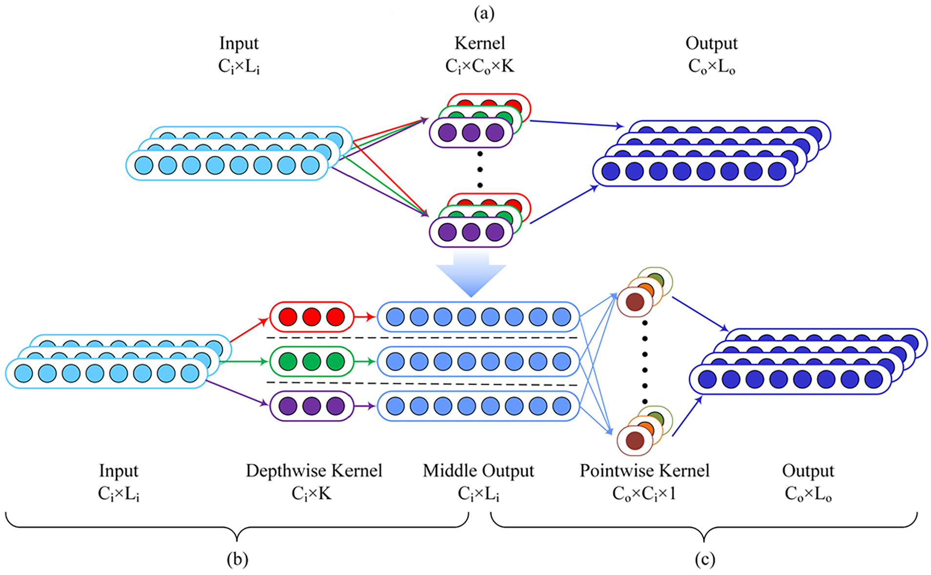
(a) Conventional convolution is replaced by (b) depthwise convolution and (c) pointwise convolution.

In 1D convolution, assuming that the size of the input feature graph is $L_{i}$ , the number of input channels is $C_{i}$ , the number of output channels is $C_{o}$ with kernel size $K$ , and disregarding the calculation amount caused by bias, the calculation amount of the convolution layer is given by:

\begin{matrix} F_{CONV} = L_{i} \times K \times C_{i} \times C_{o} \end{matrix}

(1)

In conventional convolution methods, each kernel needs to be convolved with all the input channels, whereas in deep convolution, each convolution kernel only needs to be convolved with one input channel, and then a point-by-point convolution is used to extract cross-channel features. Similarly, neglecting the parameters and calculation amount caused by the bias, the number of parameters can be calculated using the following formula:

F_{Dw} = L_{i} \times K \times C_{i} + L_{i} \times C_{i} \times C_{o}

(2)

By replacing the convolution kernels, the reduction ratio of the number of calculations is as follows:

\frac{L_{i} \times K \times C_{i} + L_{i} \times C_{i} \times C_{o}}{L_{i} \times K \times C_{i} \times C_{o}} = \frac{1}{C_{o}} + \frac{1}{K}

(3)

As shown in the formula, the computation amount of depthwise separable convolutions is usually K times less than that of conventional standard convolution, which can effectively reduce the reasoning time and memory consumption.

Network pruning

Network pruning is a key technique for compressing deep learning models and effectively reducing memory size and bandwidth requirements. In neural networks, certain parameters are considered redundant and contribute less to the final results. In the early 1990s, trimming techniques were developed to reduce the size of trained networks without requiring retraining.²¹ This allows pruned models to be run with less inference time and similar accuracy to prepruned models, facilitating the use of neural networks in resource-constrained environments such as embedded systems.

Pruning techniques are categorized into connection and filter pruning based on the pruned element type.²² In connection pruning, the weight of each channel is evaluated, and the channels with the least influence are removed. In filter pruning methods, as shown in Figure 2, the convolution kernels are directly reduced as they determine the number of output channels. The primary challenge is to identify filters with minimal impact on the accuracy of the pruning parameters while maintaining model precision. In addition, the output of the intermediate layer affects the subsequent input. Therefore, the input parameters of the full connection layer and BN layer should be clipped accordingly.

Figure 2.

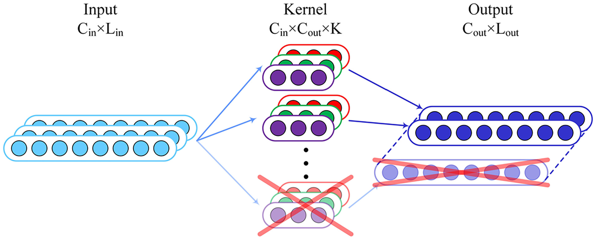
Filter pruning.

Knowledge distillation

After pruning, the neural network must be retrained to compensate for any performance degradation. Knowledge distillation²³ is a widely used technique in which a student model is trained using the soft labels generated by the teacher model. This enables the student model to gain knowledge and expertise from the teacher model.

The detailed distillation process is shown in Figure 3. The process begins with the creation of the teacher model, which is characterized by complexity and an unlimited number of parameters. The student model, which has a simpler structure and fewer parameters, is then trained using hard labels from the dataset and soft labels based on the output of the teacher model. After knowledge distillation, the performance of the student model can be improved to approach that of the teacher model so that a large network can be transformed into a small one.

Figure 3.

Knowledge distillation.

Proposed method of multi-stage pruning distillation

Deep learning models have shown remarkable performance in fault diagnosis. However, the deployment and application of edge-intelligence platforms still face challenges in terms of computational power and real-time requirements. Therefore, a lightweight fault diagnosis model based on depthwise separable convolutions is proposed in this study. Pruning techniques are applied to further reduce the computation of depthwise separable convolutions, and a novel knowledge distillation method is introduced to help fine-tune and recover the accuracy during the pruning process. In addition, a multi-stage approach is chosen to minimize accuracy loss during the pruning process and maximize the effect of knowledge distillation.

Lightweight model structure based on depthwise separable convolution

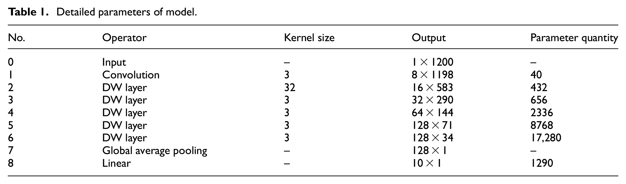
To classify the fault modes of bearings, the construction of a neural network model based on depthwise separable convolution is presented in this section. The details of the model parameters are listed in Table 1. The size of the input signal is $1 \times 1, 200,$ and before using depthwise separable convolutions to extract features, a regular 3 × 3 conventional convolution is applied to increase the feature extraction ability and robustness of the model by increasing the number of feather channels. The main body of the DW layer comprises a depthwise and pointwise convolution. The initial DW layer is set to a kernel size of 32 to facilitate feature extraction on a wider scale, reduce noise interference, and reduce data requirements. Batch normalization layers are added after each convolution to allow more flexible network parameter settings and improve the fitting speed of the network. As the neural network deepens, the number of channels continues to increase, resulting in an excessive number of feature maps. Therefore, each DW layer is followed by a maximum pooling operation. Before the final classification using a fully connected layer, a global average pooling layer is introduced to extract global contextual information, improve the generalization ability of the model, and prevent overfitting.

Table 1.

Detailed parameters of model.

No.	Operator	Kernel size	Output	Parameter quantity
0	Input	–	1 × 1200	–
1	Convolution	3	8 × 1198	40
2	DW layer	32	16 × 583	432
3	DW layer	3	32 × 290	656
4	DW layer	3	64 × 144	2336
5	DW layer	3	128 × 71	8768
6	DW layer	3	128 × 34	17,280
7	Global average pooling	–	128 × 1	–
8	Linear	–	10 × 1	1290

Pruning depthwise separable convolutions

The conventional 1D-CNN structure can be denoted by $F^{(i)} \in R^{c_{i + 1} \times c_{i} \times k}$ as the convolutional kernel of layer i, where k is the kernel size. The input can be denoted as $X^{(i)} \in R^{c_{i} \times l_{i}}$ and the output as

\begin{matrix} Y_{c, :}^{(i)} = \sum_{j = 1}^{c_{i}} X_{j, :}^{(i)} * F_{c, j, :}^{(i)}, c \in {1, 2, \dots, c_{i + 1}} \end{matrix}

(4)

where “*” represents the convolution. Pruning techniques that eliminate specific convolutional kernels reduce the output depth and only affect the input size of the subsequent layers.

For a depthwise separable convolution, the input is divided into $c_{i}$ groups. Assuming $D^{(i)} \in R^{1 \times c_{i} \times k}$ is the $i$ -th depthwise kernel, the middle output tensor $M$ is given by

\begin{matrix} M_{c, :}^{(i)} = X_{c, :}^{(i)} * D_{c, 1, :}^{(i)}, c \in {1, 2, \dots, c_{i}} \end{matrix}

(5)

Then the pointwise convolution is applied, whose kernel can be denoted as $P^{(i)} \in R^{c_{i + 1} \times c_{i} \times 1}$ . The output of the layer is evaluated as

\begin{matrix} Y_{c, :}^{(i)} = \sum_{j = 1}^{c_{i}} M_{c, :}^{(i)} * P_{c, j, 1}^{(i)}, c \in {1, 2, \dots, c_{i + 1}} \end{matrix}

(6)

In contrast to the pruning operations performed on conventional convolutions, deeply separable volumes affect both the input and output layers. More specifically, with respect to the i-th depth-separable convolution, parameterized by $(D^{(i)}, P^{(i)})$ , each depthwise filter $D_{c, 1, :}^{(i)}$ processes the input feature map $X_{c, :}^{(i)}$ , obtained by the pointwise convolution of the ( $i - 1)$ -th layer with the filter $P_{c, :, 1}^{(i - 1)}$ . To summarize, the filtered pruning pattern between the i-th deep convolution and the (i−1)-th point convolution was the same, as shown in Figure 4. Similar to the pruning of standard convolutions, after pruning the filters in $D^{(i)}$ and $P^{(i)}$ , the corresponding kernels in the following layers must also be pruned.

Figure 4.

Pruning a depthwise separable convolution.

Using a pretrained module, the constraint relationships between all filters are evaluated and then categorized for those slated for pruning into the same group for subsequent operations.²⁴ For each filter marked for pruning, a binary mask variable is introduced that corresponds to the weight tensor of the layer in terms of size and shape. During pruning, the mask variables are modified by masking the weights with the smallest magnitude by zero to determine which of the weights are excluded from participating in the forward execution. As the kernels in each group have the same pruning patterns, their mask variables should be modified as a whole.

Mean contrastive knowledge distillation

According to their distillation objectives, knowledge distillation methods can be divided into two categories: feature alignment and logit alignment. As the unimportant channel parameters are set to zero during pruning, aligning the output features in the hidden layer of the student and teacher models is difficult. Therefore, the contrastive distillation method was used to align the logits.

Mean contrastive knowledge distillation (MCKD) is based on creating a representation learning model by identifying instances that are similar or dissimilar, as shown in Figure 5. Using this model, the instances are transformed into a projection space, where similar instances are closer to each other and dissimilar instances are farther away. Consider two deep neural networks, the teacher model $f^{T}$ and a student $f^{S}$ . Let $x$ be the network input, and $f^{T} (x)$ and $f^{S} (x)$ be the outputs (logits) of the last layer of the network, respectively. Let $q$ represent the training samples and $p^{i}$ represent all other samples classified differently from $q$ . The outputs $f^{S} (q)$ and $f^{T} (q)$ are taken to form a pair of positive samples, whereas the outputs $f^{S} (q)$ and $f^{T} (p^{i})$ form negative sample pairs. The distance between positive and negative sample pairs helps develop a loss function, as follows:

\begin{array}{l} L (q, α, β; f) = m a x (0, | | f^{S} (q) - f^{T} (q) | |_{2}^{2} \\ - \frac{α}{N} \sum_{0}^{N - 1} | | f^{S} (q) - f^{T} (p^{i}) | |_{2}^{2} + β) \end{array}

(7)

where $α$ represents the distance attenuation of the negative sample pairs and $β$ represents the distance expectation of the positive and negative samples. When the distance measurement of positive sample pairs is large or the distance measurement of negative sample pairs is small, the loss function L increases to optimize the model parameters so that positive sample pairs are pushed closer together and negative sample pairs are pushed apart.

Figure 5.

Mean contrastive knowledge distillation.

Acknowledging the ongoing parameter shifts during training, standard contrastive learning methods require randomly generating normally distributed vectors with equivalent dimensions to serve as negative samples and then using a momentum update strategy to gradually update the negative samples.²⁵ The advantage of contrastive distillation learning is that the parameters of the teacher model do not need to change during the distillation process. Therefore, the teacher model is used to obtain a sample dictionary before the distillation process is officially performed. When constructing negative samples, the sample dictionary is queried directly, which considerably improves the effectiveness of the negative samples.

Multi-stage pruning distillation interleaving network

As a significant parameter gap exists between the model before and after pruning, there may be an irrecoverable drop in performance, particularly at high pruning ratios. Gradual pruning²⁶ is a straightforward and powerful method that progressively prunes the parts of a model with smaller weights until the desired sparsity level is reached. Gradual pruning effectively reduces the parameter gap between the model before and after each pruning iteration, resulting in better performance compared to a one-shot pruning approach. In this study, the principle of gradual pruning was adhered to while accounting for the previously discussed constraints. In gradual pruning, a portion of the weights are pruned every $Δ t$ iterations while the model is trained to maintain its accuracy. The pruning ratio after every $Δ t$ iterations is as follows:

\begin{matrix} r_{t} = r_{e} + (r_{b} - r_{e}) {(1 - \frac{t}{n Δ t})}^{3}, t \in {0, Δ t, \dots, n Δ t} \end{matrix}

(8)

where $r_{b}$ and $r_{e}$ represent the initial and final pruning ratios, respectively, and $n$ represents the number of iterations required for the pruning procedure. In each iteration, the mask variable is updated by summing the absolute values of the associated filter elements and removing the smaller elements from the ratio calculated with the formula.

When choosing a teacher model to be paired with a particular student model, there is a tendency to favor the models with higher complexity and better performance. However, evidence shows that this is not always the optimal case. Instead, if the teacher model becomes sufficiently large, the accuracy of the guided student model may decrease.²⁷ To explain this phenomenon, several possible reasons can be cited: the teacher becomes so complex that students no longer have enough capacity to mimic their behavior; and the teacher becomes more confident in the data, making their logits (soft targets) less soft, weakening the effectiveness of knowledge transfer through matching soft targets. For this reason, using the previously pruned model as a teacher to guide the accuracy recovery of the pruned model may not work well because the size difference between the models before and after pruning is too large.

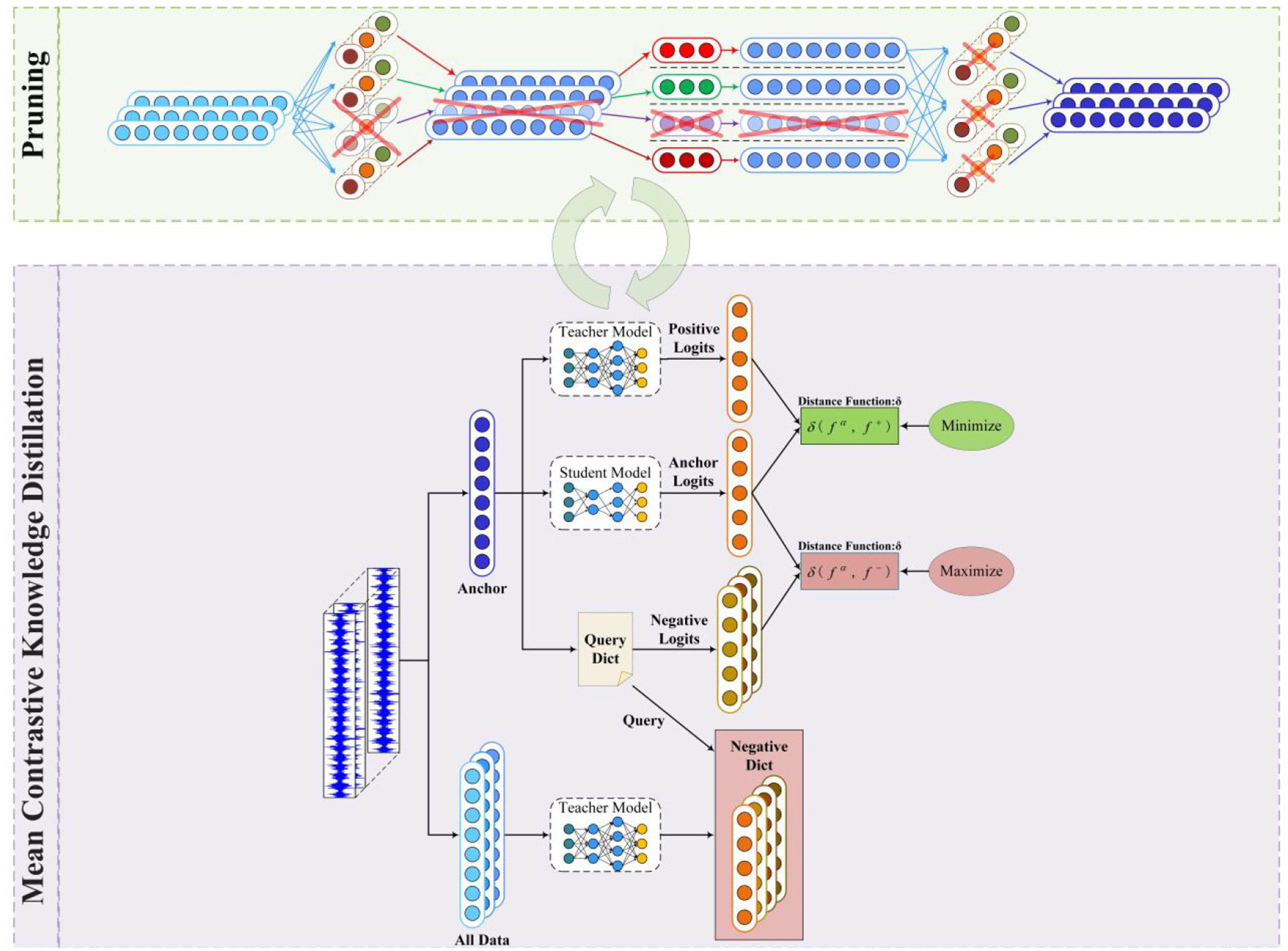
Therefore, in this study, knowledge distillation is not applied post pruning but rather incorporated into the pruning process as a fine-tuning method. The gradual pruning principle is extended to multiple stages to obtain a more precise pruning path when dealing with depthwise separable structures. Assuming that a pretrained model (pruning ratio 0.0) needs to be pruned at a ratio of $r_{f}$ , the entire procedure is divided into $S$ small stages, where gradual pruning is applied at each stage where $r_{f} / s$ of the filters are pruned. In multi-stage pruning, as the total pruning ratio is divided into each stage evenly, the differences in the model structure before and after each stage are acceptable. Therefore, the parameter gap can be effectively bridged by using the pruned model from the ( $i - 1)$ -th stage as a teacher to guide the accuracy recovery after pruning in the $i$ -th stage. The alternating network process of multi-stage pruning distillation is shown in Figure 6. The detailed steps of the proposed method are shown in Algorithm 1.

Figure 6.

Multi-stage pruning distillation alternating network.

Algorithm 1: Multi-stage Pruning Distillation Network
Input: pretrained model $M$ , final compression ratio $r_{f}$ , number of stages $S$ , pruning epochs $E_{p}$ , pruning interval $t$ , and distillation epochs $E_{d}$ Data: Training set $D$ For $s = 1, 2, 3, \dots, S - 1$ do Update teacher model $M^{T}$ with $M$ Obtain model’s kernel groups ${W^{1}, W^{2}, \dots, W^{G}}$ Obtain model’s filter index set ${I^{1}, I^{2}, \dots, I^{G}}$ Calculate begin ratio $r_{b} = s r_{f} / S$ and ending ratio $r_{e} = (s + 1) r_{f} / S$ For $t = 0, 1, . ., E_{p}$ do If $t$ is multiple of $t$ then Calculate pruning ratio $r_{t}$ by Eq. 8 Let the set of unpruned weights $T = {}$ For $g = 1, 2, \dots, G$ do For each index $i$ in $I^{g}$ , calculate its score $\sum_{w \in W^{g}} AbsSum (w_{i, :, :, :})$ Remove the indices with the smallest score from $I^{g}$ until reaching the pruning ratio $r_{t}$ in the $g$ -th group Add ${w_{i, :, :, :} \| \forall i \in I^{g}, w \in W^{g}}$ into $T$ Set weights to 0 except for those in $T$ Train the parameters of model $M$ in $T$ on $D$ Obtain a logit dictionary by $M^{T}$ For $t = 0, 1, . ., E_{d}$ do For $d$ in $D$ do Query negative logit in the sample dictionary Obtain positive logit by $M^{T}$ Obtain anchor logit by $M$ Calculate the Loss by Eq. 7 Train the parameters of model $M$ in $T$ through the loss Output: compressed model $M$

Algorithm 1: Multi-stage Pruning Distillation Network

Input: pretrained model

M

, final compression ratio

r_{f}

, number of stages

S

, pruning epochs

E_{p}

, pruning interval

t

, and distillation epochs

E_{d}

Data: Training set

D

For

s = 1, 2, 3, \dots, S - 1

do
Update teacher model

M^{T}

with

M

Obtain model’s kernel groups

{W^{1}, W^{2}, \dots, W^{G}}

Obtain model’s filter index set

{I^{1}, I^{2}, \dots, I^{G}}

Calculate begin ratio

r_{b} = s r_{f} / S

and ending ratio

r_{e} = (s + 1) r_{f} / S

For

t = 0, 1, . ., E_{p}

do
If

t

is multiple of

t

then
Calculate pruning ratio

r_{t}

by Eq. 8
Let the set of unpruned weights

T = {}

For

g = 1, 2, \dots, G

do
For each index

i

I^{g}

, calculate its score

\sum_{w \in W^{g}} AbsSum (w_{i, :, :, :})

Remove the indices with the smallest score from

I^{g}

until reaching the pruning ratio

r_{t}

in the

g

-th group
Add

{w_{i, :, :, :} | \forall i \in I^{g}, w \in W^{g}}

into $T$
Set weights to 0 except for those in

T

Train the parameters of model

M

T

D

Obtain a logit dictionary by

M^{T}

For

t = 0, 1, . ., E_{d}

do
For

d

D

do
Query negative logit in the sample dictionary
Obtain positive logit by

M^{T}

Obtain anchor logit by

M

Calculate the Loss by Eq. 7
Train the parameters of model

M

T

through the loss
Output: compressed model

M

Fault diagnosis experiments using the proposed method

Experimental environment

To verify the proposed method’s effectiveness, experiments were conducted on two bearing fault datasets. The models were trained and deployed on an NVIDIA Jetson Nano,²⁸ a leading platform for AI at the edge. This compact, powerful computer, equipped with a graphics processing unit (GPU), can run multiple neural networks in parallel while consuming only 5 W power. Another advantage is that the Jetson Nano is compatible with the Jet-Pack Software Development Kit (SDK), which has libraries for deep learning and computational acceleration. It contains a quad-core ARM A57 processor operating at 1.43 GHz, a powerful 128-core Maxwell GPU, and a 4 GB 64-bit LPDDR4.

A cross-validation method was used to facilitate parameter tuning and feature selection. Each dataset was randomly divided into a training and a test set in a 1:1 ratio. The training dataset was further divided into ten folds, with nine folds used for training and one used for validation. During the training process, the number of training epochs was set to 90, and a cross-entropy loss function was used to optimize the parameters. The learning rate was initialized at 0.1 and then reduced by a factor of 0.1 every 30 epochs. This process was repeated 10 times, and the hyperparameters for the optimal model were determined based on all 10 trained models. Finally, the model was retrained with the optimal hyperparameters on the entire training dataset, and its generalization performance was evaluated on the test dataset.

To ensure the accuracy and reliability of the model evaluations, a series of standardized procedures were followed. After determining the optimal hyperparameters, five independent experiments were conducted for each model to assess its accuracy under stable conditions. The accuracy of each model was demonstrated through confidence intervals that reflect not only the accuracy of the model but also the stability and reliability of the model’s performance under specific hyperparameter settings. With this approach, the reported model accuracies are ensured to not only perform well during training but also maintain a high generalization ability when confronted with new data.

First experiment with Paderborn University (PU) bearing fault datasets under multiple operating conditions

Datasets description

The data were provided by the Paderborn University (PU) Data Center.²⁹ The experimental test rig is shown in Figure 7. The data were collected under different operating conditions by adjusting the rotational speed of the drive system, radial force on the bearings, and load torque on the drive system. This resulted in three different operating conditions, which are listed in Table 2. Each operational condition included five health conditions: normal, inner race faults (in two degrees of severity), and outer race faults (in two degrees of severity). Their health conditions are summarized in Table 3. During data acquisition, the data were sampled at a frequency of 64 kHz, and 200 samples were acquired for analysis, each comprising 1200 data points.

Figure 7.

Test rig.

Table 2.

Operating conditions.

No.	Rotational speed (rpm)	Load torque (Nm)	Radial force (N)	Name of states
1	900	0.7	1000	N09_M07_F10
2	1500	0.7	400	N15_M07_F04
3	1500	0.1	1000	N15_M01_F10

Table 3.

Five health conditions of the bearings.

Health condition	Bearing	Damage (mm)	Category label
Normal	K004	–	0
Inner fault 1	KI21	≤2	1
Inner fault 2	KI19	>2	2
Outer fault 1	KA04	≤2	3
Outer fault 2	KA16	>2	4

Experiment results

The baseline models were trained from scratch and compressed using the proposed method, which was repeated using data of three operating conditions. After the compression ratio reached 0.75, the rate of decline in the diagnostic accuracy accelerated significantly. Therefore, a model with a compression ratio of 0.75 was selected as the main reference for comparison. To reflect the feasibility and effectiveness of our method, conventional convolutional models with the same structure (Model 1), baseline models before compression (Model 2), and compressed models with 0.5 and 0.75 of filters pruned were compared in terms of parameter quantity, computational complexity (FLOPs), mean accuracy, and prediction time under three operating conditions. The results are summarized in Table 4.

Table 4.

Comparison of the different models on PU datasets.

Models	Params	FLOPs	Accuracy	Prediction time (ms)
Model1	86,925	14.72M	99.51% ± 0.46%	21.44 ± 0.45
Model2	30,157	4.32M	99.47% ± 0.61%	19.51 ± 0.65
Proposed method_0.5	8265	1.33M	99.07% ± 0.48%	10.73 ± 0.35
Proposed method_0.75	2431	0.45M	98.20% ± 0.52%	6.20 ± 0.13

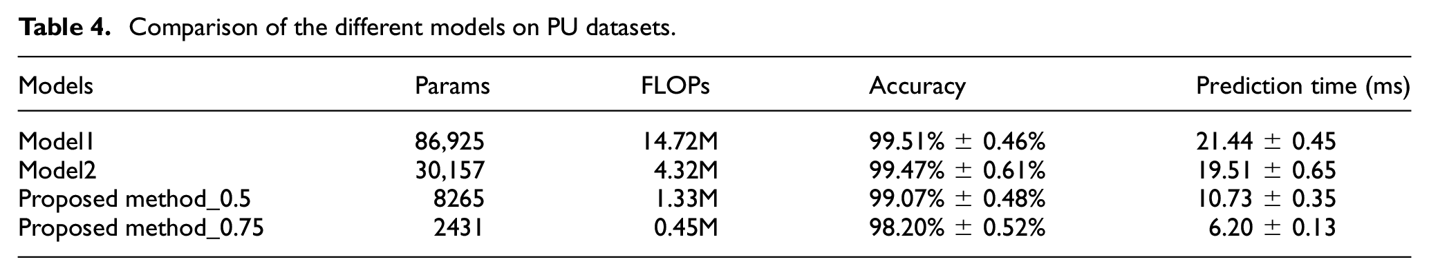
Applying deep separable convolution can reduce the parameter count of conventional convolution models to 35.17% and the computational complexity to 29.35%, with almost no loss in accuracy. With a pruning of 0.5, our compression method based on multi-stage pruning and distillation could further reduce the parameter count to 26.83% and the computational complexity to 30.72%. The final accuracy was 99.07%, which is only a decrease of 0.4% compared to the accuracy before compression. Further compression reduces the number of parameters but leads to a more significant loss of accuracy. Taking the models with a pruning ratio of 0.75 as an example, their confusion matrices and dimension reduction features were processed with t-distributed stochastic neighbor embedding (t-SNE),³⁰ as shown in Figure 8. The lightweight network constructed in this study can effectively complete the bearing fault diagnosis tasks and completely separate the fault features, while saving computational power with minimal accuracy loss.

Figure 8.

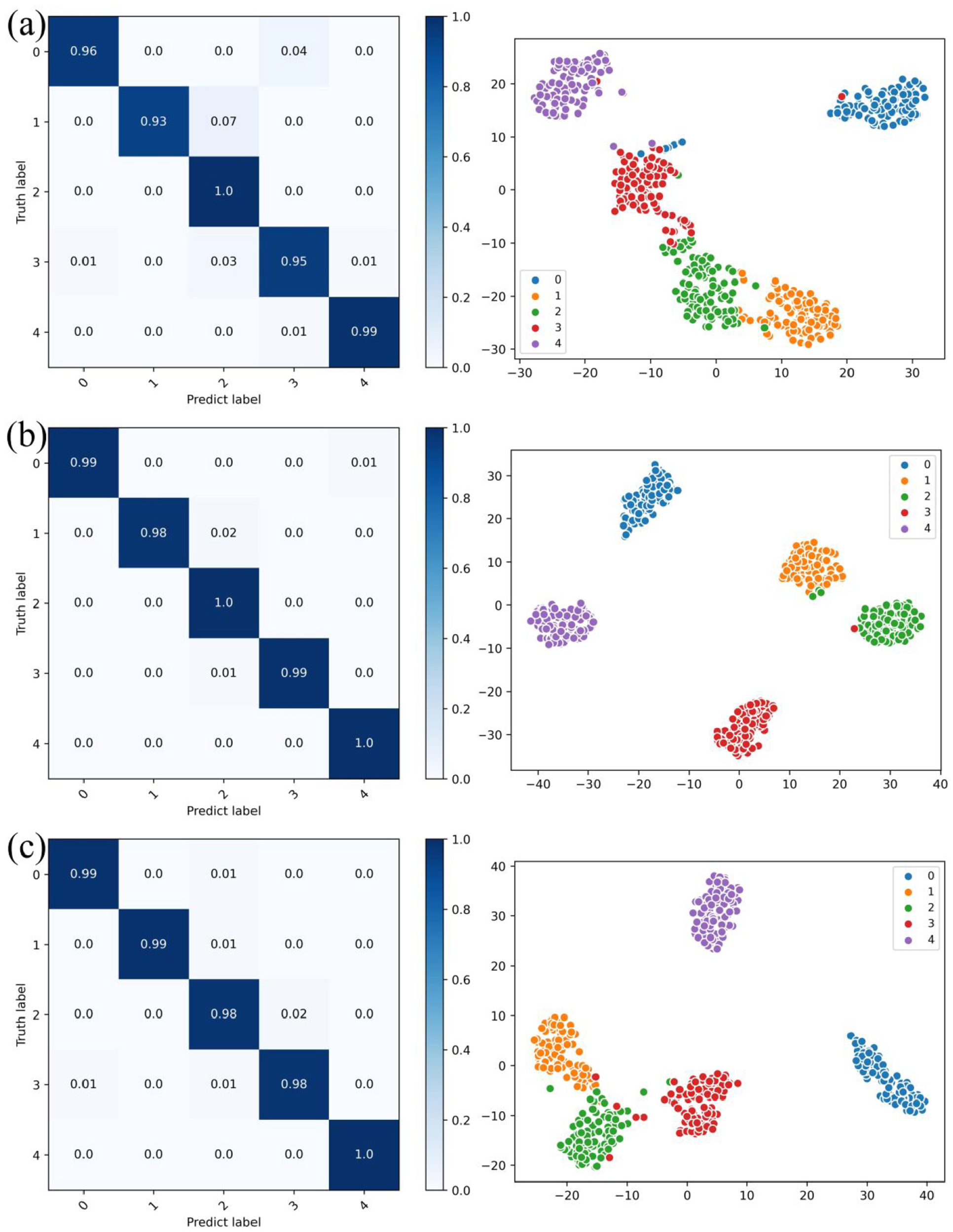
Confusion matrices and t-SNE for three operating states: (a) N09_M07_F10, (b) N15_M07_F04, and (c) N15_M01_F10.

Effectiveness of multi-stage pruning and distillation

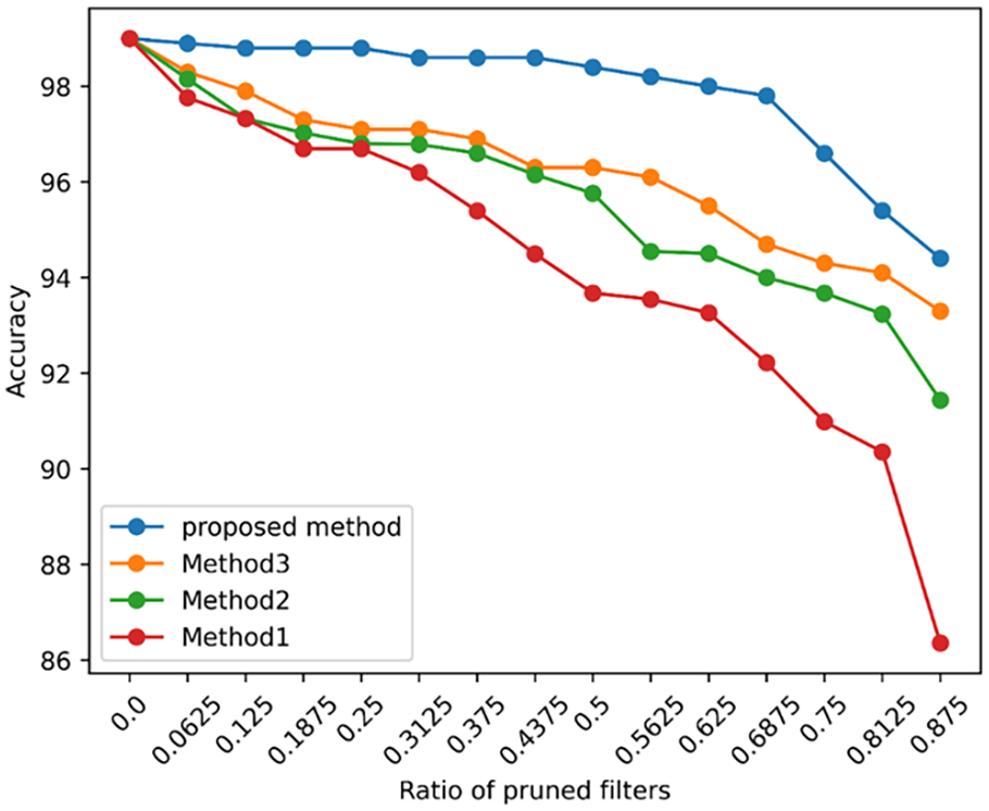
When compressing a model, the results often differ owing to pruning and distillation strategies. Experiments were conducted to determine how the different strategies affect the performance, as listed in Table 5. More specifically, in Method 1, the model is pruned to the target ratio in one shot, and accuracy is restored by classical knowledge distillation. In Method 2, 1/16 of the filters are pruned in one stage until the target ratio is reached; then, classical knowledge distillation is performed, which takes the baseline model as the teacher. Method 3 replaces the classical knowledge distillation in Method 2 with the mean contrastive knowledge distillation proposed in this study. Compared to Method 3, the proposed method performs MCDK in each stage and takes the model of the previous stage as the teacher model. Each method is trained on the data from the initial operating condition, and the changes in accuracy are shown in Figure 9.

Table 5.

Different compression strategies.

Component	Method1	Method2	Method3	Proposed method
Pruning	√
Multi-stage pruning		√	√	√
KD	√	√
MCKD			√
Multi-stage-MCKD				√

Figure 9.

Comparison of the different strategies on PU datasets.

The comparison of Method 1 and Method 2 reveals a significant difference that increases with the pruning ratio. This indicates that the application of gradual multistage pruning can effectively reduce the accuracy loss compared to one-shot pruning. The results from Method 2 and Method 3 reveal that the MCKD proposed in this study outperforms the classical method, improving the accuracy after pruning. The accuracy decrease of the proposed method is much slower and smoother than that of Method 3, which benefited from the multistage strategy that bridges the parameter gap between the pruned and unpruned models. The downward trend in accuracy became more pronounced after a pruning ratio of 0.75. This is because only one filter remains in each convolutional layer, which significantly reduces the feature extraction ability. In general, the proposed method outperformed the other strategies in all stages, indicating its effectiveness and superiority.

To compare the effects of different pruning stage quantities on the model, we conducted diagnostic tests using four distinct pruning ratios, with the results depicted in Figure 10. The figure reveals that, under higher pruning rates, methods with more pruning stages can maintain greater accuracy. Furthermore, it is evident that the accuracy difference between the 16-stage and 32-stage methods is negligible. Considering that a greater number of pruning stages requires more time for fine-tuning, the 16-stage pruning configuration was ultimately chosen based on a comprehensive evaluation of diagnostic performance and time consumption.

Figure 10.

Comparison of the different compression stages on PU datasets.

Next, to observe the impact of varying pruning stages from another perspective, we plotted the changes in training loss under different pruning stages, as shown in Figure 11. In this experiment, we controlled for the same total number of epochs to negate the influence of varying fine-tuning cycles corresponding to different pruning stages. The figure first demonstrates that each pruning process leads to a significant increase in training loss. Additionally, it can be observed that models with more pruning stages experience smaller increases in training loss and exhibit less fluctuation compared to those with fewer pruning stages. Finally, models with more pruning stages also exhibit better convergence, likely due to the smaller structural changes before and after each pruning iteration. Knowledge distillation, serving as the fine-tuning method, can more effectively extract and transfer knowledge under these conditions.

Figure 11.

The change of training loss with epochs in different compression stages on PU datasets.

To more intuitively illustrate the changes occurring in models with different pruning stages, we take the pointwise convolution in the third DW layer as an example. With the remaining number of convolutional kernels fixed at 0.25, the l_2 norm, representing the sum of the absolute values of all parameters within the kernels, is employed. Figure 12 displays the remaining convolutional kernels under different pruning stages. It is clear that methods with fewer pruning stages exhibit a distinct difference in the remaining kernels compared to those with more pruning stages. Considering that more pruning stages entail fewer kernels being pruned in a single stage, the selection process becomes more meticulous, resulting in smaller accuracy drops due to individual pruning events. The knowledge distillation used for fine-tuning allows the remaining kernels to retain the original model’s knowledge to a greater extent. This ensures that the kernels selected by methods with more stages are more representative and play a more significant role in model inference.

Figure 12.

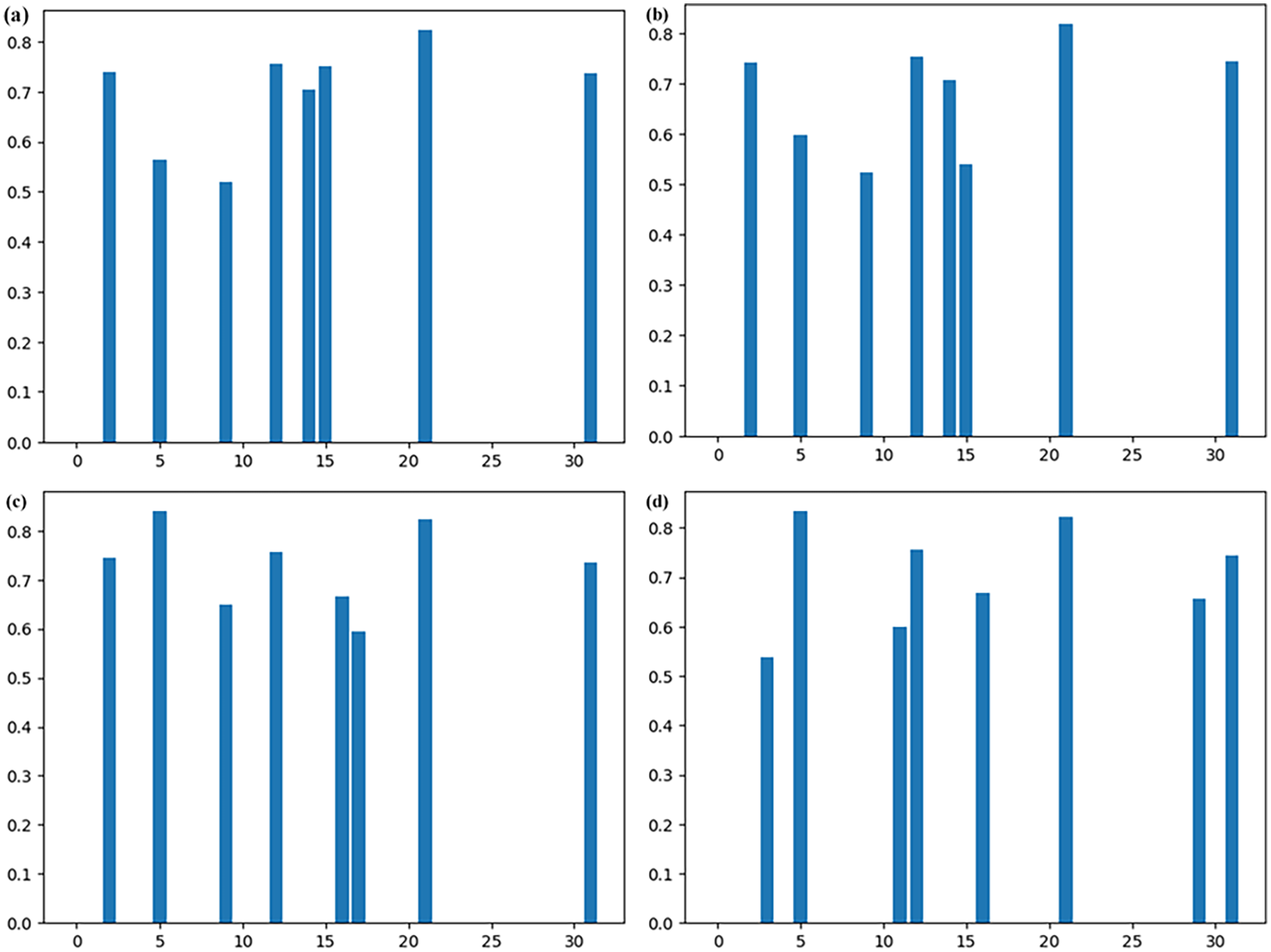
Pointwise convolutional kernels of the third DW layers in models on PU datasets compressed within (a) 32 stages, (b) 16 stages, (c) 8 stages, and (d) 4 stages.

To validate the advantages of the proposed method, three of the most effective lightweight models were applied to the dataset. The details of the three networks are explained below: Model 3³¹ is based on a stacked inverted residual convolution neural network that applies depthwise separable convolution and a linear bottleneck. Model 4³² includes squeeze-excitation modules within an inverted residual convolutional neural network. Model 5¹⁵ uses weight-sharing multiscale convolution and inverse separable convolution and eliminates useless network structures by an adaptive pruning technique. Each model was trained with datasets from three operating states, and the mean accuracy was considered as the final result. Figure 13 shows the comparison results, the details of which are listed in Table 6.

Figure 13.

Calculation cost and mean accuracy of the different models on PU datasets.

Table 6.

Comparison with other methods on PU datasets.

Models	Params	FLOPs	Accuracy	Prediction time (ms)
Proposed method_0.5	8265	1.33M	99.07% ± 0.48%	10.73 ± 0.35
Proposed method_0.75	2431	0.45M	98.20% ± 0.52%	6.20 ± 0.13
Model3	33,000	20M	97.93% ± 0.57%	27.41 ± 0.53
Model4	25,000	2.5M	98.38% ± 0.43%	15.37 ± 0.26
Model5	13,000	2.5M	99.04% ± 0.51%	13.29 ± 0.46

The proposed method leads to a reduction in complexity as it benefits from a depthwise separable convolution and a high pruning ratio. Based on diagnostic accuracy alone, our method with 0.5 filters pruned is the best. Model 3 might be overfitted because of over-parameterization, so the accuracy cannot be further improved. Model 4 loses a lot of important information because of the heavy use of convolutions, with the stride set to 2. Model 5 has the second highest accuracy, but its parameters are redundant owing to the multiscale feature convolution. The proposed method has a more refined pruning and distillation process, resulting in a small loss of accuracy. If it is further compressed, the advantages of complexity can be enhanced with acceptable loss of accuracy. To summarize, the proposed network outperforms the other three contemporary lightweight models in terms of both complexity and accuracy.

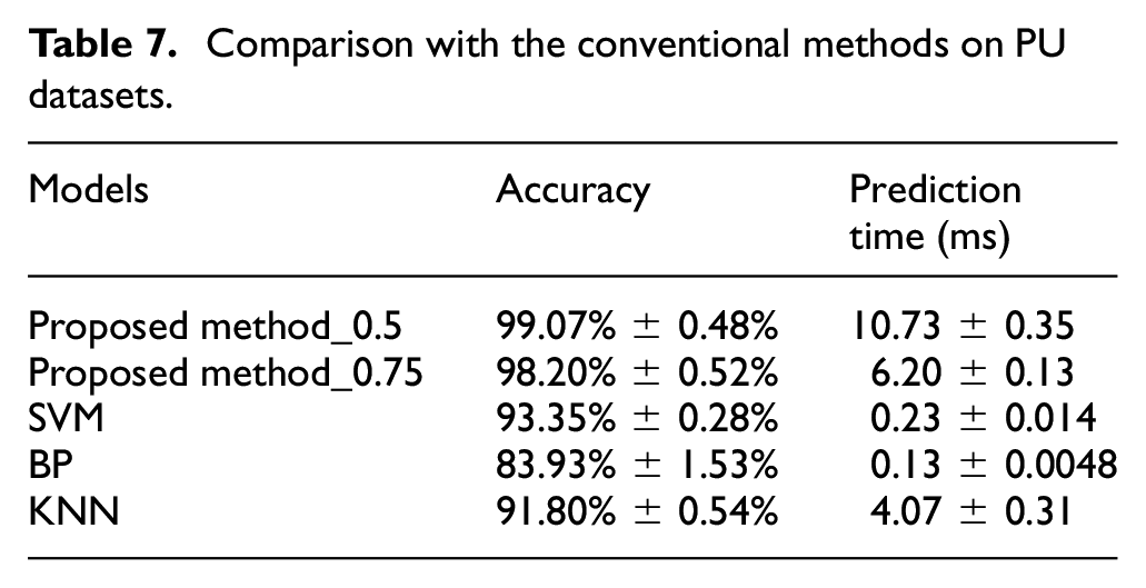
Conventional methods represent an important benchmark as the cornerstone of the diagnostic field. To fully assess the effectiveness of a fault diagnosis method, it is not sufficient to compare it with state-of-the-art methods. Therefore, the proposed method was compared with three conventional fault diagnosis methods: support vector machine (SVM), backpropagation (BP), and K-nearest neighbor (KNN), in terms of model accuracy and model inference time under the same experimental conditions. Table 7 lists a comparison of the experimental results. The experimental results show that although the conventional methods can provide fast prediction results owing to their relatively simple computational process, their prediction accuracy is significantly lower compared to the proposed method, and the inference time of our method can meet the requirements of real edge applications. This experiment has clearly demonstrated the potential and advantages of the proposed method in the field of modern fault diagnosis.

Table 7.

Comparison with the conventional methods on PU datasets.

Models	Accuracy	Prediction time (ms)
Proposed method_0.5	99.07% ± 0.48%	10.73 ± 0.35
Proposed method_0.75	98.20% ± 0.52%	6.20 ± 0.13
SVM	93.35% ± 0.28%	0.23 ± 0.014
BP	83.93% ± 1.53%	0.13 ± 0.0048
KNN	91.80% ± 0.54%	4.07 ± 0.31

The choice of hyperparameters has a significant effect on the performance of the model, and analyzing the process uncertainty helps us to better understand the stability and reliability of the model in practical applications. To verify the stability and accuracy of the fault diagnosis method under different hyperparameter thresholds, a hyperparameter experiment was designed and conducted. By adjusting the two key hyperparameters α and β in the distillation loss function and plotting contour plots reflecting the relationship between the hyperparameters and the accuracy of the model, the performance of the model was carefully analyzed under different hyperparameter configurations. Figure 14 shows the results of the experiment. The models with different compression ratios achieved the maximum accuracy of the model with similar values of the hyperparameters. With increasing threshold value, the model accuracy roughly shows the trend of increasing and then decreasing, while the hyperparameters do not drastically decrease when they are far from the optimal values, indicating that our proposed method has a certain degree of stability.

Figure 14.

Model accuracy of the different hyperparameters on PU datasets: (a) proposed method_0.5 and (b) proposed method_0.75.

Second experiment on a dataset with different rotational speeds

Datasets description

For the second experiment, a specially designed motor-bearing test bench consisting of a motor, two rotors, and a bearing seat was used. A type 1A314E vibration acceleration sensor was affixed to the upper surface of the bearing seat and operated at a sampling frequency of 25.6 kHz. To evaluate the robustness of the proposed method, the complexity of the dataset was increased. Table 8 lists the bearing health conditions included in this dataset: normal condition and three types of faults (roller, inner race, and outer race) with different degrees of damage (0.2, 0.4, and 0.6 mm). Each health condition comprises 200 samples, with 1200 data points each, conducted at four different rotational speeds (1000, 1500, 2000, and 2500 rpm).^33,34

Table 8.

Ten health conditions of the bearings.

Health condition	Label
Normal	0
Roller element fault with a degree of 0.2 mm	1
Roller element fault with a degree of 0.4 mm	2
Roller element fault with a degree of 0.6 mm	3
Inner race fault with a degree of 0.2 mm	4
Inner race fault with a degree of 0.4 mm	5
Inner race fault with a degree of 0.6 mm	6
Outer race fault with a degree of 0.2 mm	7
Outer race fault with a degree of 0.4 mm	8
Outer race fault with a degree of 0.6 mm	9

Experimental results

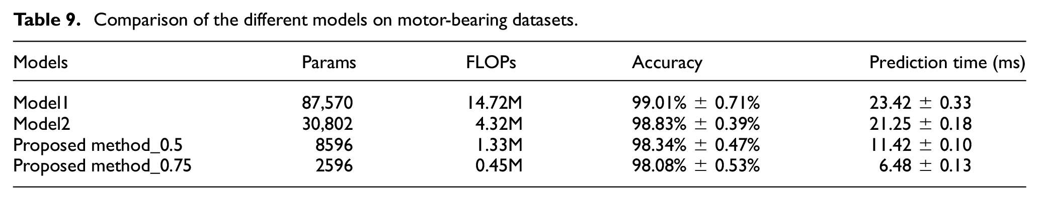
The models were trained on datasets with four different rotational speeds and then compressed using our method. Similar to experiment 1, it was compared with the other models, and the results are listed in Table 9. Additional labels slightly increase the accuracy loss with depthwise separable convolution. However, our method remained effective, losing only 0.49% accuracy when 0.5 of the filters were pruned. The confusion matrices and dimension reduction features for models pruned at a ratio of 0.75 processed by t-SNE are shown in Figure 15. Slight overlap occurs within the same fault type; the other fault types were clearly separated. This demonstrates the excellent performance of the proposed method in terms of accuracy and complexity.

Table 9.

Comparison of the different models on motor-bearing datasets.

Models	Params	FLOPs	Accuracy	Prediction time (ms)
Model1	87,570	14.72M	99.01% ± 0.71%	23.42 ± 0.33
Model2	30,802	4.32M	98.83% ± 0.39%	21.25 ± 0.18
Proposed method_0.5	8596	1.33M	98.34% ± 0.47%	11.42 ± 0.10
Proposed method_0.75	2596	0.45M	98.08% ± 0.53%	6.48 ± 0.13

Figure 15.

Effectiveness of multi-stage pruning and distillation

The effectiveness of the proposed method is explained in more detail in this section. The different compression methods used for comparison are the same as those described in the previous section, and the results of the data from the first operating condition are shown in Figure 16. As in experiment 1, the proposed method resulted in a slower and smoother accuracy loss during compression. As show in Figures 17 to 19, the performance gap between the 16-stage and 32-stage methods is similarly minuscule, yet both notably surpass the efficacy of their 4-stage and 8-stage methods.

Figure 16.

Comparison of the different strategies on motor-bearing datasets.

Figure 17.

Comparison of the different compression stages on motor-bearing datasets.

Figure 18.

The change of training loss with epochs in different compression stages on motor-bearing datasets.

Figure 19.

Pointwise convolutional kernels of the third DW layers in models on motor-bearing datasets compressed within (a) 32 stages, (b) 16 stages, (c) 8 stages, and (d) 4 stages.

The results for this dataset compared with the state-of-the-art lightweight models mentioned above are shown in Figure 20 and Table 10. As the model structure remains unchanged, the proposed method retains its complexity. The fault features become more complex owing to the 10 different label sets in the dataset. Model 3 took advantage of its parameter quantity and showed the best diagnostic performance. Model 5 had the same accuracy as the proposed method, which can be attributed to its multiscale feature extraction capability. As the accuracy is excellently maintained after compression, the diagnostic capability of the proposed method also reaches the same level as that of Model 3 when the pruning ratio is 0.5. In terms of both complexity and precision, the proposed network outperforms three contemporary lightweight models for bearing fault diagnosis.

Figure 20.

Calculation cost and mean accuracy of the different models on motor-bearing datasets.

Table 10.

Comparison with other methods on motor-bearing datasets.

Models	Params	FLOPs	Accuracy	Prediction time (ms)
Proposed method_0.5	8265	1.33M	98.34% ± 0.47%	11.42 ± 0.10
Proposed method_0.75	2596	0.45M	98.08% ± 0.53%	6.48 ± 0.13
Model3	33,000	20M	98.41% ± 0.44%	29.17 ± 0.61
Model4	25,000	2.5M	98.18% ± 0.51%	14.73 ± 0.31
Model5	13,000	2.5M	98.34% ± 0.48%	14.15 ± 0.27

Next, the same experimental procedure as for the first dataset was repeated to evaluate the performance of the proposed fault diagnosis method. The results are listed in Table 11 and shown in Figure 21. A comparative analysis with the conventional diagnostic techniques, SVM, BP, and KNN, again highlights the advantages of our method in terms of accuracy and inference speed. In the hyperparameter-tuning experiments, the stability of the model accuracy was investigated by a limited number of parameter variations, and it was found that the model maintained a relatively stable performance even when the parameter values deviated from the optimal points. These results are further evidence of the reliability and applicability of the proposed method to different datasets.

Table 11.

Comparison with the conventional methods on motor-bearing datasets.

Models	Accuracy	Prediction time (ms)
Proposed method_0.5	98.34% ± 0.47%	11.42 ± 0.10
Proposed method_0.75	98.08% ± 0.53%	6.48 ± 0.13
SVM	91.93% ± 0.57%	0.59 ± 0.069
BP	74.42% ± 1.41%	0.16 ± 0.028
KNN	89.23% ± 0.31%	7.37 ± 0.52

Figure 21.

Model accuracy of the different hyperparameters on motor-bearing datasets: (a) proposed method_0.5 and (b) proposed method_0.75.

Conclusions

By using a lightweight design and model compression, a feasible solution to the problems of poor real-time performance and high computation time in bearing fault diagnosis on edge-computing platforms was provided in this study. A neural network based on depth-separable convolution was developed to predict the health conditions of bearings using bearing vibration signals as input. A constrained gradual pruning technique was applied to the trained model to remove redundant parameters, and knowledge distillation was used to allow the pruned model to benefit from the expertise condensed and transferred from the unpruned model. The entire compression process is divided into multiple stages to minimize the loss of accuracy in pruning and increase the effectiveness of distillation. The experimental results confirm that the proposed method can achieve high accuracy in fault diagnosis with a compact model structure. In the future, the plan is to optimize the proposed method using edge computing platform hardware to further improve the real-time performance of the bearing fault diagnosis model, making it more suited for practical applications.

Despite these remarkable results, our approach still faces some challenges. First, the model did not perform well under variable operating conditions or high-noise environments. Consequently, further research is needed to improve its adaptability to anomalous inputs. Secondly, the interpretability of the model may be reduced by the use of compression and distillation techniques. Future work should aim to improve the model’s transparency to clarify the decision-making process. In addition, the ability of the model to generalize to different industrial environments and bearing types needs to be further investigated. To address these limitations, future research should focus on increasing the robustness of the model, improving its interpretability, and expanding the scenarios in which it can be used to enable a wider range of applications.

Footnotes

Handling Editor: Aarthy Esakkiappan

Author contributions

Conceptualization, Linlin Ren; Methodology, Xiaoming Li and Hongbo Ma; Software, Linlin Ren and Xiaoming Li; Validation, Hongbo Ma and Guowei Zhang; Formal Analysis, Guowei Zhang and Song Huang; Investigation, Hongbo Ma; Resources, Guowei Zhang; Data Curation, Song Huang and Ke Chen; Writing – Original Draft Preparation, Linlin Ren and Hongbo Ma; Writing – Review & Editing, Linlin Ren and Xiaoming Li; Visualization, Hongbo Ma; Supervision, Weijie Yue and Xiaoqing Wang; Project Administration, Xiaoming Li and Hongbo Ma; Funding Acquisition, Hongbo Ma. All authors have read and agreed to the published version of the manuscript.

Declaration of conflicting interests

The author(s) declared no potential conflicts of interest with respect to the research, authorship, and/or publication of this article.

Funding

The author(s) disclosed receipt of the following financial support for the research, authorship, and/or publication of this article: This work was supported by the National Key Research and Development Program of China (2022YFB3706803).

ORCID iD

Hongbo Ma

Data availability statement

The data presented in this study are available on request from the corresponding author.

References

Alotaibi

A survey on industrial Internet of Things security: requirements, attacks, AI-based solutions, and edge computing opportunities. Sensors 2023; 23: 7470.

, et al. Multi-level federated learning based on cloud-edge-client collaboration and outlier-tolerance for fault diagnosis. Meas Sci Technol 2023; 34: 125148.

Fei

Zhang

Edge-to-cloud IIoT for condition monitoring in manufacturing systems with ubiquitous smart sensors. Sensors 2022; 22: 5901.

Zhang

Deng

Zheng

, et al. Development of an edge computing-based cyber-physical machine tool. Robot Comput Integr Manuf 2021; 67: 102042.

Qiao

Wang

A tool wear monitoring and prediction system based on multiscale deep learning models and fog computing. Int J Adv Manuf Technol 2020; 108: 2367–2384.

Wang

Huang

, et al. Efficient data reduction at the edge of industrial internet of things for PMSM bearing fault diagnosis. IEEE Trans Instrum Meas 2021; 70: 1–12.

IEEE Committee Report. Report of large motor reliability survey of industrial and commercial installations. IEEE Trans Ind Appl 1987; 23: 153–158.

Zhang

Wang

, et al. Signals hierarchical feature enhancement method for CNN-based fault diagnosis. Adv Mech Eng 2022; 14: 16878132221125019.

Ruicong

Zhongtian

, et al. Unsupervised adversarial domain adaptive for fault detection based on minimum domain spacing. Adv Mech Eng 2022; 14: 16878132221088647.

10.

Zhu

Chen

Meng

, et al. A wide kernel CNN-LSTM-based transfer learning method with domain adaptability for rolling bearing fault diagnosis with a small dataset. Adv Mech Eng 2022; 14: 16878132221135745.

11.

Chen

Ran

Deep learning with edge computing: a review. Proc IEEE 2019; 107: 1655–1674.

12.

Han

Pool

Tran

, et al. Learning both weights and connections for efficient neural network. Adv Neural Inf Process Syst 2015; 28: 1135–1143.

13.

Wang

, et al. Compressed channel-based edge computing for online motor fault diagnosis with privacy protection. IEEE Trans Instrum Meas 2023; 72: 1–12.

14.

Liu

Shen

, et al. Learning efficient convolutional networks through network slimming. In: Proceedings of the IEEE international conference on computer vision, Venice, Italy, 22–29 October 2017, pp.2736–2744. New York: IEEE.

15.

Ding

Qin

Wang

, et al. Lightweight multiscale convolutional networks with adaptive pruning for intelligent fault diagnosis of train bogie bearings in edge computing scenarios. IEEE Trans Instrum Meas 2023; 72: 1–13.

16.

Liu

Wang

, et al. Network lightweight method based on knowledge distillation is applied to RV reducer fault diagnosis. Meas Sci Technol 2023; 34: 095110.

17.

Madaan

Shin

Hwang

SJ.

Adversarial neural pruning with latent vulnerability suppression. In: International conference on machine learning, PMLR, Virtual, 13–18 July 2020, pp.6575–6585.

18.

Howard

Zhu

Chen

Mobilenets: efficient convolutional neural networks for mobile vision applications. arXiv preprint arXiv: 1704.04861, 2017.

19.

Agarap

. Deep learning using rectified linear units (relu). arXiv preprint arXiv:1803.08375, 2018.

20.

Ioffe

Szegedy

. Batch normalization: Accelerating deep network training by reducing internal covariate shift. arXiv 2015[J]. arXiv preprint arXiv:1502.03167, 2015.

21.

Reed

Pruning algorithms - a survey. IEEE Trans Neural Netw 1993; 4: 740–747.

22.

Kadav

Durdanovic

, et al. Pruning filters for efficient ConvNets[J]. arXiv preprint arXiv: 1608.08710, 2016.

23.

Hinton

Vinyals

Dean

Distilling the knowledge in a neural network. arXiv preprint arXiv: 1503.02531, 2015.

24.

Lee

Chan

, et al. Pruning depthwise separable convolutions for mobilenet compression. In: 2020 international joint conference on neural networks (IJCNN), Glasgow, UK, 19–24 July 2020, pp.1–8. New York: IEEE.

25.

Fan

, et al. Momentum contrast for unsupervised visual representation learning. In: Proceedings of the IEEE/CVF conference on computer vision and pattern recognition, Seattle, WA, USA, 13–19 June 2020, pp.9729–9738. New York: IEEE.

26.

Zhu

Gupta

. To prune, or not to prune: exploring the efficacy of pruning for model compression[J]. arXiv preprint arXiv:1710.01878, 2017.

27.

Mirzadeh

Farajtabar

, et al. Improved knowledge distillation via teacher assistant. Proc AAAI Conf Artif Intell 2020; 34: 5191–5198.

28.

NVIDIA. Jetson Nano. NVIDIA, https://www.nvidia.com/en-us/autonomous-machines/embedded-systems/jetson-nano/product-development/ (accessed 18 September 2024).

29.

Lessmeier

Kimotho

Zimmer

, et al. Condition monitoring of bearing damage in electromechanical drive systems by using motor current signals of electric motors: a benchmark data set for data-driven classification. Proc Eur Conf Progn Health Manag Soc 2016; 3: 1–17.

30.

Maaten

Hinton

Visualizing data using t-SNE. J Mach Learn Res 2008; 9: 2579–2605.

31.

Yao

Liu

Yang

, et al. A lightweight neural network with strong robustness for bearing fault diagnosis. Measurement 2020; 159: 107756.

32.

Liu

Chen

, et al. A rolling bearing fault diagnosis method using novel lightweight neural network. Meas Sci Technol 2021; 32: 125102.

33.

Zhang

Kong

, et al. Adaptive multispace adjustable sparse filtering: a sparse feature learning method for intelligent fault diagnosis of rotating machinery. Eng Appl Artif Intell 2023; 120: 105847.

34.

Zhang

Kong

Wang

, et al. Multi-source partial domain adaptation method based on pseudo-balanced target domain for fault diagnosis. Knowl Based Syst 2024; 284: 111255.

Lightweight intelligent fault diagnosis method based on a multi-stage pruning distillation interleaving network

Abstract

Keywords

Introduction

Theoretical background of lightweight networks and model compression

Depthwise separable convolutions

Network pruning

Knowledge distillation

Proposed method of multi-stage pruning distillation

Lightweight model structure based on depthwise separable convolution

Pruning depthwise separable convolutions

Mean contrastive knowledge distillation

Multi-stage pruning distillation interleaving network

Fault diagnosis experiments using the proposed method

Experimental environment

First experiment with Paderborn University (PU) bearing fault datasets under multiple operating conditions

Datasets description

Experiment results

Effectiveness of multi-stage pruning and distillation

Second experiment on a dataset with different rotational speeds

Datasets description

Experimental results

Effectiveness of multi-stage pruning and distillation

Conclusions

Footnotes

Author contributions

Declaration of conflicting interests

Funding

ORCID iD

Data availability statement

References