Multi-fault bearing diagnosis under time-varying conditions using Empirical Wavelet Transform,Gaussian mixture model,and Random Forest classifier

Abstract

Bearing faults can cause heavy disruptions in machinery operation, which is why their reliable diagnosis is crucial. While current research into bearing fault analysis focuses on analyzing vibration data under constant working conditions, it is important to consider the challenges that arise when machinery runs at variable speeds, which is usually the case. This article proposes a multistage classifier for diagnosing bearings under time-variable conditions. We validate our method using vibration signals from five bearing health states, including a combined fault case. Our approach involves decomposing the signals using Empirical Wavelet Transform and computing temporal and frequency domain attributes. We use the Expectation-Maximization Gaussian mixture model for optimization concerns to identify relevant parameters and train the Random Forest classifier with the selected features. Our method, evaluated using the Polygon Area Metric, has demonstrated high effectiveness in diagnosing bearings under time-variable conditions. Our approach offers a promising solution that efficiently addresses speed variability and combined fault recognition issues.

Introduction

Bearing is a crucial component of rotary machines, but it is also highly susceptible to failure. ¹ Therefore, accurate diagnosis of bearings is essential to ensure the functionality of rotary machines ² and the safety of employees. ³ As a result, many researchers have focused on this issue and developed new diagnosis strategies based on various condition monitoring techniques, including vibration, current, acoustic emissions, and temperature. ⁴ Signals are extensively used for bearing diagnosis due to their effectiveness in detecting and analyzing bearing faults. ⁵ The vibration signals provide crucial information related to bearing health and fault conditions, making them a valuable source for fault diagnosis. Various studies have demonstrated the significance of vibration signals in bearing fault detection and diagnosis, ⁶ this approach is favored because it effectively captures system conditions and degradation characteristics through vibration datasets. ⁷ However, the primary challenge lies in accurately extracting fault features from these datasets. Over recent decades, plenty of signal-processing methods have been developed to address various failure modes, characteristics, and data types. These methods aim to achieve early fault detection by eliminating unwanted components such as interference noise.^8–10 Common time-domain techniques include autoregressive moving average, dimensionless factor, and singular value decomposition. Similarly, frequency-domain methods such as Fourier transform and spectral kurtosis have been widely applied.^11–13 Additionally to these techniques, a wide range of time-frequency analysis tools are adopted for this matter. The Empirical Wavelet Transform (EWT) approach is the best method for analyzing this type of signal, as it allows for simultaneous insight into the time and frequency domains. ¹⁴ In Wang et al., ¹⁵ the EWT was employed to handle the complexity of bearing fault feature extraction under changing speeds. Many researchers have embraced the EWT technique, including Dong et al., ¹⁶ Xu and Ma, ¹⁷ Xi et al., ¹⁸ and Hariharan et al., ¹⁹ due to its potential to overcome the shortcomings of well-performing procedures such as Empirical Mode Decomposition (EMD), which suffers from the mode-mixing problem ²⁰ and the lack of theoretical foundation, ²¹ and the time-varying spectral amplitude method because of its complexity and computational cost, parameter sensitivity. However, these methods have certain limitations. They can be time-consuming due to their extensive and intricate feature extraction processes. Moreover, the feature extraction itself is complex and requires substantial resources. It is important to note that extracting features for a specific fault detection technique applies solely to that particular issue and may not be suitable for a different fault diagnosis technique, especially when dealing with conditions that vary over time. After extracting the signal modes, calculating the statistical parameters is an essential step. However, some features may be irrelevant and deceptive. Hence, feature selection becomes crucial to keep only the discriminative parameters for training the classification model. Optimization algorithms can yield meaningful results in feature selection, and they have become a significant phase in the diagnostic process. For instance, in Wu et al., ²² the grey wolf optimization algorithm (GOA) delivered good results by flexibly learning important parameters of joint distribution adaption. Similarly, in Wang et al., ²³ the Grasshopper Optimization Algorithm (GOA) improved the Support Vector Machine (SVM) classifier’s pattern recognition capabilities and demonstrated its usefulness in diagnosing rolling bearing faults. Additionally, in Van et al., ²⁴ Particle Swarm Optimization ensured a higher accuracy of the proposed Least-Squares wavelet support vector machine (LSWSVM) by selecting the most relevant features. However, it is worth noting that all the mentioned algorithms were applied at constant speeds, while bearings usually operate under time-varying conditions. To address this, in Imane et al., ²⁵ the Clan-based Cultural Algorithm (CCA) was applied in bearing diagnosis using time-varying vibration data. It provided promising results with accurate classification, but the treated cases did not include combined faults. Besides these techniques, deep learning algorithms have shown promising performance in bearing fault detection. However, while they have shown high accuracy, there are some disadvantages to using them. Deep learning algorithms require significant computational resources, including high-performance computing systems and large amounts of memory, to train and optimize the models.^26,27 Also, they require large amounts of labeled data to train the models effectively.^26,28 This can be a challenge in applications where data is insufficient or labeling is difficult or time-consuming. In addition, deep learning algorithms are often considered “black boxes” because they are difficult to interpret and understand.^26,28 They are often criticized for their limited interpretability, making it difficult to understand how the model arrives at its predictions. This can be a disadvantage in applications where transparency and interpretability are important, such as in safety-critical systems.

This article discusses the diagnosis of bearings in time-varying settings, including combination defects, with five bearing health states, including combined defects using machine learning. First, we analyze the vibration signatures using the EWT to extract the AM-FM modes. Next, we compute statistical features in both time and frequency domains. To address the high computational cost of the wrapper optimization class and the independence of the filter class’s results from the clustering algorithms, ²⁹ we applied the Expectation-Maximization-based Gaussian mixture model (EM-GMM) clustering algorithm to select only the features capable of distinguishing the exact number of classes. The final step involves supplying the selected attributes to the Random Forest (RF) classifier to train a robust model using only the discriminative elements. The article is structured as follows: Sections “Preprocessing and feature extraction based on Empirical Wavelet Transform,”“Fault identification with optimization algorithm based on expectation maximization Gaussian mixture model,” and “Fault patterns based on Random forest” provide the theoretical background on EWT, EM-GMM, and RF, respectively. Section “Experimental study” describes the data used, and the process, and presents the results and discussions. We conclude with a summary of our findings.

Preprocessing and feature extraction based on Empirical Wavelet Transform

Gilles ³⁰ proposed the EWT intending to construct adaptive wavelets capable of extracting finite AM-FM components (modes) $f_k(t)$ of the signal $f(t)$ , such as:

$$f(t)=\sum _{k=0}^N{f}_k(t)$$

(1)

The core concept of EWT involves creating bandpass filters on each $\Lambda n$ with $\Lambda n=[{\omega }_n,{\omega }_{n+1}]$ and $U_{n=1}^N{\Lambda }_n=[0,,,\pi ]$ . The process is summarized in Figure 1, it begins by computing the local maxima from the Fourier spectrum of $f(t)$ , followed by dividing the spectrum into segments based on the boundaries identified at the center of two subsequent peaks. Finally, empirical wavelets are constructed to break down the signal into its constituent parts.

Figure 1.

Flowchart of EWT.

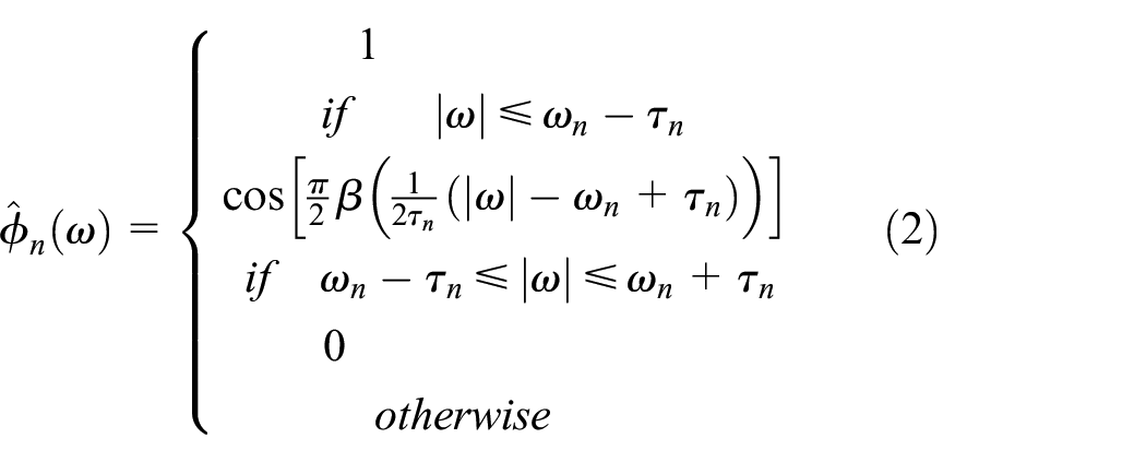
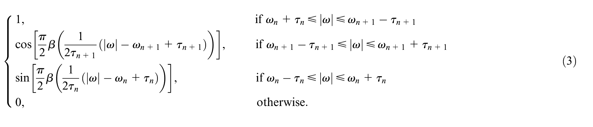
Expressions 2 and 3 define the empirical scaling function and the empirical wavelets, respectively.

$$\begin{array}{c}\multicolumn{1}{c}{{\hat{\varphi }}_n\left(\omega \right)=\{\begin{array}{c}1\hfill \\ \multicolumn{1}{c}{\mathrm{if}\left|\omega \right|\le {\omega }_n-{\tau }_n}\\ \multicolumn{1}{c}{\cos \left[\frac{\pi }{2}\beta \left(\frac{1}{2{\tau }_n}(\left|\omega \right|-{\omega }_n+{\tau }_n)\right)\right]}\\ \multicolumn{1}{c}{\mathrm{if}{\omega }_n-{\tau }_n\le \left|\omega \right|\le {\omega }_n+{\tau }_n}\\ \multicolumn{1}{c}{0}\\ \multicolumn{1}{c}{\mathrm{otherwise}}\end{array}}\end{array}$$

(2)

$$\begin{array}{c}\multicolumn{1}{c}{\{\begin{array}{c}1,\mathrm{if}{\omega }_n+{\tau }_n\le \left|\omega \right|\le {\omega }_{n+1}-{\tau }_{n+1}\hfill \\ \multicolumn{1}{c}{\cos \left[\frac{\pi }{2}\beta \left(\frac{1}{2{\tau }_{n+1}}(\left|\omega \right|-{\omega }_{n+1}+{\tau }_{n+1})\right)\right],\mathrm{if}{\omega }_{n+1}-{\tau }_{n+1}\le \left|\omega \right|\le {\omega }_{n+1}+{\tau }_{n+1}}\\ \multicolumn{1}{c}{\sin \left[\frac{\pi }{2}\beta \left(\frac{1}{2{\tau }_n}(\left|\omega \right|-{\omega }_n+{\tau }_n)\right)\right],\mathrm{if}{\omega }_n-{\tau }_n\le \left|\omega \right|\le {\omega }_n+{\tau }_n}\\ \multicolumn{1}{c}{0,\mathrm{otherwise}.}\end{array}}\end{array}$$

(3)

Among numerous functions that satisfy the properties, expression 4 is the most commonly used.

$$\beta \left(x\right)=x^4(35-84x+70x^2-20x^3)$$

(4)

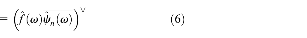
The EWT ${\mathcal{W}}_f^{\epsilon }(n,t)$ is defined as for the classical WT, the coefficients are obtained by the inner product of the original signal and the empirical wavelets. ³⁰

$${\mathcal{W}}_f^{\epsilon }(n,t)=〈f,{\psi }_n〉=\int f\left(\tau \right)\overline{{\psi }_n(\tau -t)}d\tau$$

(5)

$$={\left(\hat{f}\left(\omega \right)\overline{{\hat{\psi }}_n\left(\omega \right)}\right)}^{\vee }$$

(6)

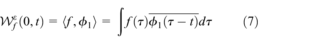
The approximation coefficients are calculated using equation (7).

$${\mathcal{W}}_f^{\epsilon }(0,t)=〈f,{\varphi }_1〉=\int f\left(\tau \right)\overline{{\varphi }_1(\tau -t)}d\tau$$

(7)

So the signal’s empirical modes $f_k$ can be calculated as follows:

$$f_0\left(t\right)={\mathcal{W}}_f^{\epsilon }(0,t)*{\varphi }_1\left(t\right)$$

(8)

$$f_k\left(t\right)={\mathcal{W}}_f^{\epsilon }(k,t)*{\psi }_k\left(t\right)$$

(9)

The original signal can be reconstructed using the equation (10).

$$f\left(t\right)={\mathcal{W}}_f^{\epsilon }(0,t)*{\varphi }_1\left(t\right)+\sum _{n=1}^N{\mathcal{W}}_f^{\epsilon }(n,t)*{\psi }_n\left(t\right)$$

(10)

Fault identification with optimization algorithm based on expectation maximization Gaussian mixture model

Gaussian Mixture Models (GMM) are commonly applied in data mining, pattern recognition, machine learning, and statistical analysis. ³¹

GMM aims to fit the data distribution of arbitrary shapes by finding the M latent Gaussian densities given by equation (11).

$$p(x|{\mu }_i,{\Sigma }_i)=\sum _{i=1}^M{\omega }_i{p}_i(x)$$

(11)

Where ${\omega }_i$ are mixture weights and satisfy the following constraints.

$$\sum _{i=1}^M{\omega }_i=1\mathrm{and}0\le {\omega }_i\le 1$$

(12)

And,

$$P_i(x)=\mathcal{N}(x|{\mu }_i,{\Sigma }_i)$$

(13)

$\mathcal{N}$ is the Gaussian distribution and it is defined by equation (14).

$$\mathcal{N}(x|{\mu }_i,{\Sigma }_i)=\frac{1}{{(2\pi )}^{N/2}}\frac{1}{|{\Sigma }_i{|}^{1/2}}{e}^{(-\frac{1}{2}{(x-{\mu }_i)}^T{\Sigma }_i^{-1}(x-{\mu }_i))}$$

(14)

${\mu }_i$ are the mean vectors, ${\Sigma }_i$ are the covariance matrices with $i\in \{1,....,M\}$ .

The estimation of the characterizing parameters is an essential step in the GMM. The Expectation-Maximization (EM) algorithm represents an efficient tool, ³² which seeks to identify the maximum likelihood estimate. ³³

In the case of the discrete distributions, the likelihood is simply the joint probability of our data. We assume that each point is independent, and then the likelihood of all data is equal to the product of the likelihood of each data point, as explained in equation (15).

$$L(\mathrm{\Theta })=\underset{i=1}{\overset{n}{\mathrm{\Pi }}}P(x_i|\mathrm{\Theta })$$

(15)

With $\mathrm{\Theta }=\{\mu ,\Sigma \}$ We expend equation (15) as follows:

$$\underset{i=1}{\overset{n}{\mathrm{\Pi }}}P(x_i|\mathrm{\Theta })=P(x_1|\mathrm{\Theta })\times P(x_2|\mathrm{\Theta })\times \dots \times P(x_n|\mathrm{\Theta })$$

(16)

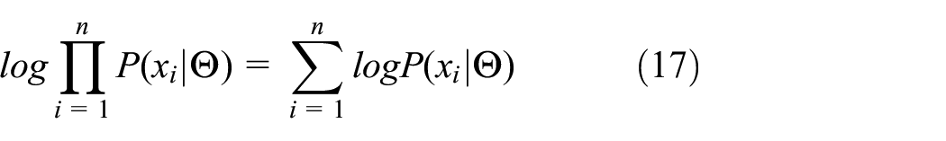
To find the maximum likelihood, we need to differentiate the equation (16). However, it is a difficult task. As a solution, we can utilize the log-likelihood to simplify this step by transforming the product into a sum, as shown in equation (17).

$$\log \underset{i=1}{\overset{n}{\mathrm{\Pi }}}P(x_i|\mathrm{\Theta })=\sum _{i=1}^n\mathrm{logP}(x_i|\mathrm{\Theta })$$

(17)

We denote $\hat{\mathrm{\Theta }}$ as the values that maximize equation (17).

$$\hat{\mathrm{\Theta }}=\mathrm{argmax}\sum _{i=1}^n\mathrm{logP}(x_i|\mathrm{\Theta })$$

(18)

Where $\mathrm{argmax}$ stands for Arguments of maxima, and the function’s argmax is the value of the domain where the function is maximized.

In our study, we will take a fresh look at this technique and utilize it in feature selection.

Fault patterns based on Random forest

Random Forest (RF) is a classifier based on trees, consisting of multiple trees generated using random vectors sampled independently from the input vector. ³⁴ The number of parameters used to determine the optimal split at each node is a subset of the total number of parameters selected randomly. ³⁵ RF uses Breiman’s Classification and Regression Tree (CART) method to determine splits in training data and generate individual trees from a newly produced bootstrap sample of the training set to ensure that they differ significantly. ³⁶ A classifier tree contains several nodes, each representing a specific condition. It takes either one or zero, resulting in two subnodes, and the variable at each node should achieve maximal homogeneity between the two resulting subnodes. This homogeneity can be quantified in various ways. For categorical classification, the Gini Index is the most popular method, and it is considered a measure of impurity. The Gini Index for node $p$ is defined by equation (19). ³⁶

$$I_P=n_P.\sum _{c=1}^C{\mathrm{\Pi }}_p(c)[1-{\mathrm{\Pi }}_p(c)]$$

(19)

Where $n_P$ refers to the total number of training instances, ${\mathrm{\Pi }}_P$ denotes the proportion of occurrences $c$ in $P$ , and $c$ represents the class. The decrease of impurity in other words the increase in homogeneity resulting from the split of $R$ and $L$ nodes can be measured by equation (20).

$$\mathrm{\Delta }I(P,L,R)=I_P-(I_L+I_R)$$

(20)

At the end, the split that maximizes $\mathrm{\Delta }I(P,L,R)$ is chosen after evaluating all alternative splits, the process is repeated until reaching the maximum depth.

In classification, each tree releases a unit vote for the most popular class, ³⁷ and then RF assigns a class for each sample by taking the majority of votes from all predictor trees.

Experimental study

Data-set description

This study is dedicated to the detection of bearing faults in varying rotational speed conditions. For this purpose, we opted for the “Bearing vibration data collected under time-varying rotational speed conditions” database, chosen for its significant value in evaluating the efficacy of various methods developed for bearing fault detection. This database provides a diverse array of vibration signals from bearings operating under a range of time-varying rotational speed conditions, rendering it an invaluable resource for assessing the performance of detection techniques in such dynamic scenarios. ³⁸

The dataset utilized in our study is a more recent iteration of the one introduced by Huang and Baddour, ³⁸ released in 2019. This updated database encompasses vibration signals collected from bearings exhibiting five distinct health states and operating under varying time-varying rotational speed conditions. Notably, each health state is subjected to two experimental conditions: specific bearing health states and variable speed conditions.

The bearing’s health conditions are:

1. Healthy

2. Faulty with an inner race defect.

3. Faulty with an outer race defect.

4. Faulty with a ball defect.

5. Faulty with combined defects on the inner race, the outer race, and a ball.

The data are acquired under:

• Increasing speed

• Decreasing speed

• Increasing then decreasing speed

• Decreasing then increasing speed

For more authenticity, three trials are repeated for each case with a sampling rate of 200,000 Hz for 10 s.

Experimental results and comparative study

The process of our proposed approach for early detection and classification is summarized in the flowchart shown in Figure 2, and it is divided mainly into three steps.

Figure 2.

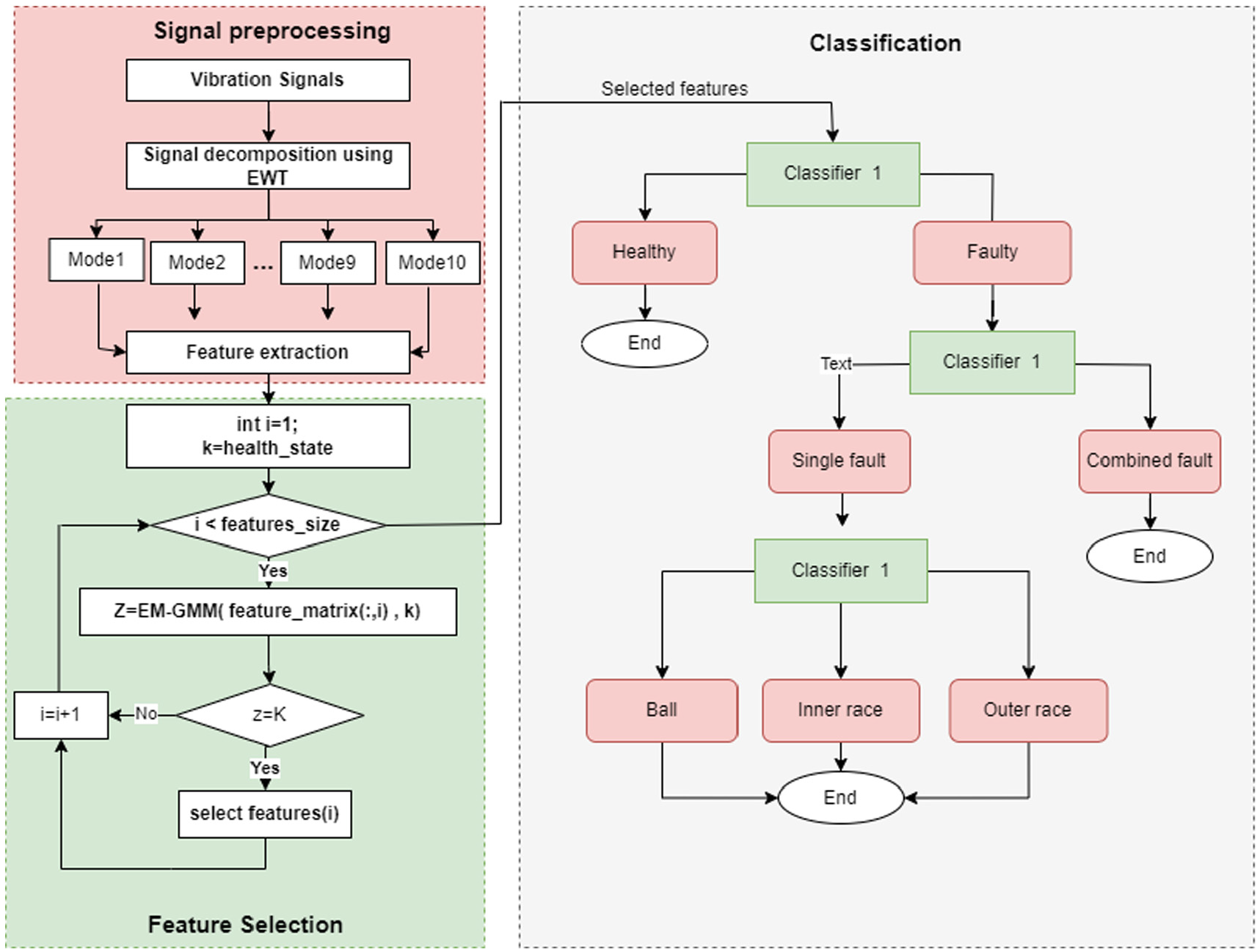
Flowchart of the proposed process.

Our procedure involves three key steps. Initially, we employ the Empirical Wavelet Transform (EWT) to meticulously extract the AM-FM modes embedded within the vibration signatures. This robust technique facilitates a precise decomposition of the signal into a predetermined number of modes. For our investigation, we deliberately selected 10 modes, as illustrated in Figure 3, this specific number of modes was chosen building upon the insights gained from our previous study, ²⁵ which utilized the same database but focused on a classification task involving three health states only instead of the current five, we extensively explored the impact of varying the number of modes extracted using Empirical Wavelet Transform (EWT). Through rigorous experimentation and comparative analysis, we found that employing 10 modes yielded satisfactory classification accuracy and performance metrics results, strategically ensuring effective encapsulation of the vibration signature’s inherent characteristics. Subsequently, we calculate a comprehensive set of features for these 10 modes, as outlined in Table 1, resulting in 170 attributes. This extensive feature set provides a nuanced comprehension of the underlying characteristics of the vibration signature, enabling us to discern subtle changes and patterns that may serve as indicative markers.

Figure 3.

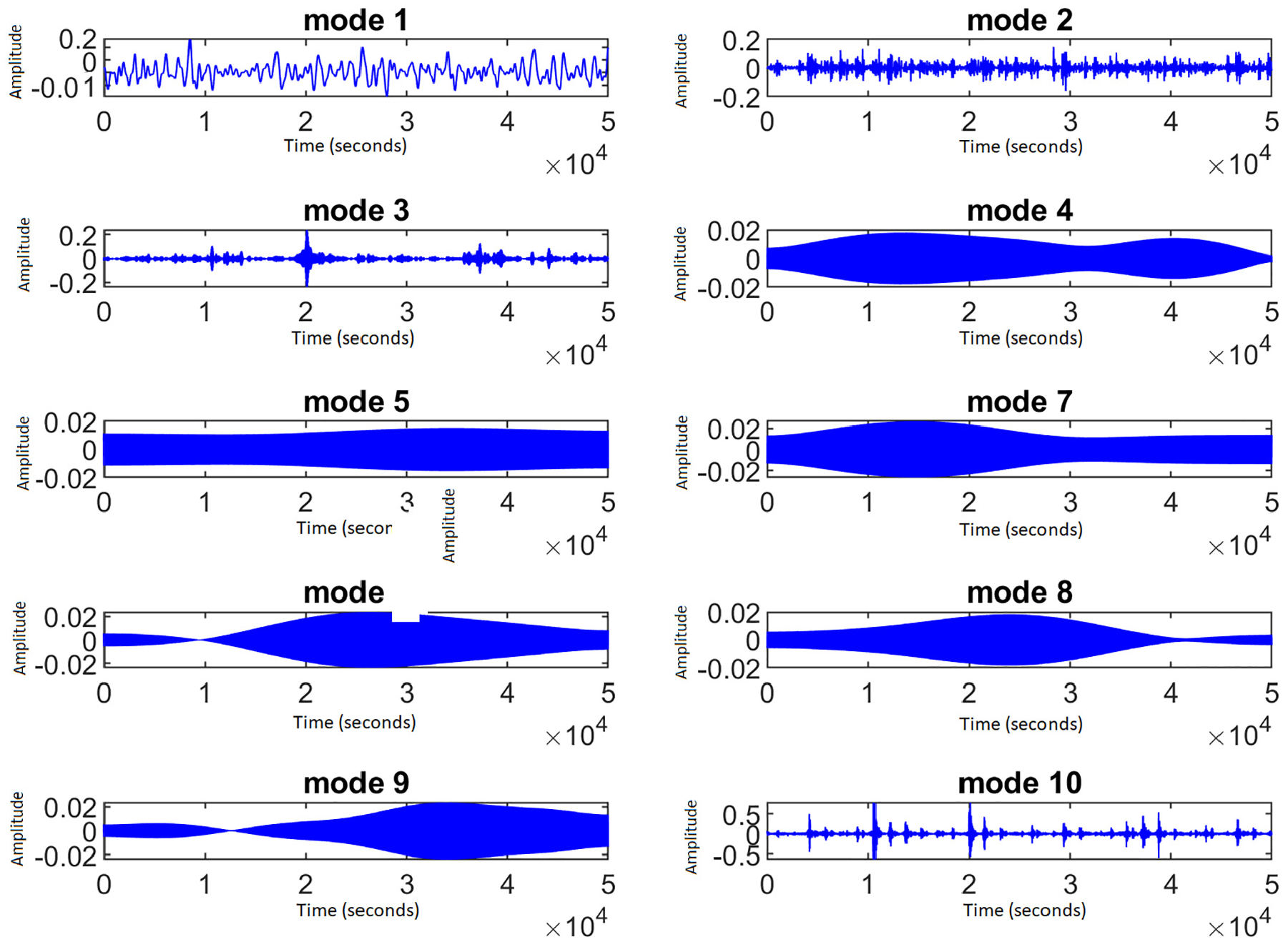
Extracted AM-FM modes using the EWT for bearing with faulty inner race.

Table 1.

Table of extracted features.

Feature	Definition	Equation/description
Maximum	The highest value in the signal.	$\mathrm{Max}=max(x)$
Minimum	The lowest value in the signal.	$\mathrm{Min}=min(x)$
Median	The middle value when the data is sorted.	Calculate the median of $x$ .
Peak to peak	The difference between the maximum and minimum values.	$\mathrm{Peak}2\mathrm{Peak}=\mathrm{Max}-\mathrm{Min}$
Root mean square	The square root of the average of the squared values.	$\mathrm{RMS}=\sqrt{\frac{1}{N}\sum _{i=1}^N{x}_i^2}$
Mean	The average value of the signal.	$\mathrm{Mean}=\frac{1}{N}\sum _{i=1}^N{x}_i$
Standard deviation	A measure of the dispersion of data points.	$\mathrm{STD}=\sqrt{\frac{1}{N}\sum _{i=1}^N{(x_i-\mathrm{Mean})}^2}$
Kurtosis	A measure of the “tailedness” of the data distribution.	$\mathrm{Kurtosis}=\frac{N\sum _{i=1}^N{(x_i-\overline{x})}^4}{{\left[\sum _{i=1}^N{(x_i-\overline{x})}^2\right]}^2}$
Crest factor	The ratio of the peak value to the RMS value.	$\mathrm{Peak}2\mathrm{RMS}=\frac{\mathrm{Max}}{\mathrm{RMS}}$
Skewness	A measure of the asymmetry of the data distribution.	$\mathrm{Skewness}=\frac{\sum _{i=1}^N{(x_i-\overline{x})}^3}{(n-1){\sigma }^3}$
Variance	The average of the squared differences from the Mean.	$\mathrm{VAR}=\frac{1}{N}\sum _{i=1}^N(x_i-\mathrm{Mean}{)}^2$
Root sum of squares	The square root of the sum of the squares of the values.	$\mathrm{Rssq}=\sqrt{\sum _{i=1}^N{x}_i^2}$
Energy	The total energy of the signal.	$\mathrm{EN}=\sum _{i=1}^N{x}_i^2$
Peak frequency	The frequency corresponding to the maximum amplitude in the spectrum.	Find the frequency at which the spectrum has its maximum value.
Mean frequency	The weighted average of the frequencies in the spectrum.	Calculate the weighted average frequency of the spectrum.
Median frequency	The frequency below which half of the energy is contained in the spectrum.	Find the frequency such that cumulative energy is 50%.
Signal-to-noise ratio (SNR)	The ratio of the signal power to noise power in decibels.	$\mathrm{SN}{R}_{\mathrm{dB}}=10·\underset{10}{\log }\left(\frac{P_s}{P_n}\right)$

In the second step of our methodology, we employ the EM-GMM clustering algorithm to pinpoint the most pertinent set of features for each of the three delineated stages, as depicted in the classification part in Figure 2. This entails a meticulous examination of the data at each level individually, identifying elements that offer optimal differentiation between the various classes. Our approach involves selecting features that precisely distinguish the specific number of groups, a visual representation of which is illustrated in the feature selection part in Figure 2. This iterative process is repeated for each stage, systematically determining the discriminative features tailored to each level. The last step is to use the three selected sets $S{F}_i$ to train three independent classifier models $\mathrm{MD}{L}_i$ using the Random Forest classifier with different classes described by $\mathrm{Labe}{l}_i$ , which will be nested as described in algorithm 1 to perform a multistage classification as depicted in the classification stage in Figure 2.

Algorithm 1. Multi-stage classification pseudo-code.

Input: $S{F}_1,S{F}_2,S{F}_3,\mathrm{Data}\_\mathrm{Test},\mathrm{Label}\_\mathrm{Test},\mathrm{MD}{L}_1,\mathrm{MD}{L}_2,\mathrm{MD}{L}_3$ Output: $\mathrm{Accuracy}$   $\mathrm{Labe}{l}_1=[\mathrm{healthy},\mathrm{faulty}]$   $\mathrm{Labe}{l}_2=[\mathrm{one}\_\mathrm{fault},\mathrm{combined}\_\mathrm{faults}]$   $\mathrm{Labe}{l}_3=[\mathrm{inner}\_\mathrm{race},\mathrm{outer}\_\mathrm{race},\mathrm{ball}]$  for $i=1:\mathrm{size}(\mathrm{data}\_\mathrm{Test},1)$ do    $\mathrm{predicted}(i)=\mathrm{MD}{L}_1(\mathrm{Data}\_\mathrm{Test}(i,S{F}_1))$   if $(\mathrm{predicted}(i)==\mathrm{faulty})$ then     $\mathrm{predicted}(i)=\mathrm{MD}{L}_2(\mathrm{Data}\_\mathrm{Test}(i,S{F}_2))$    if $(\mathrm{predicted}(i)==\mathrm{one}\_\mathrm{fault})$ then      $\mathrm{predicted}(i)=\mathrm{MD}{L}_3(\mathrm{Data}\_\mathrm{Test}(i,S{F}_3))$    end if   end if end for $\mathrm{correct}\leftarrow 0$ for $i=1:\mathrm{size}(\mathrm{Data}\_\mathrm{Test},1)$ do  if $(\mathrm{predicted}(i)==\mathrm{Label}\_\mathrm{Test}(i))$ then    $\mathrm{correct}\leftarrow \mathrm{correct}+1$  end if end for $\mathrm{Accuracy}\leftarrow \mathrm{correct}/\mathrm{size}(\mathrm{data}\_\mathrm{Test},1)$

False alarm detection using binary classification

First, we carry out a binary classification using the Random Forest algorithm for the inner race, outer race, and the ball cases with the selected features by the Gaussian Mixture Model (GMM). The outcome of this process is summarized and presented in Table 2.

Table 2.

Binary classification results.

Element	Inner race	Outer race	Ball
Accuracy	100%	100%	100%

The results of the binary classification are very accurate. In the second step, the combined fault scenario will be assessed besides healthy data, utilizing a cascade of the three classifiers, as outlined in algorithm 2. The three classifiers should detect the fault for the combined case since the three parts are defective.

Algorithm 2. Combined fault detection using binary classifiers.

Input: $\mathrm{Inner}\_\mathrm{race},\mathrm{Outer}\_\mathrm{race},\mathrm{Ball},\mathrm{Label}.$ Output: $\mathrm{Accuracy}$   $\mathbf{If}Inner\_race==defected\wedge Outer\_race==defected\wedge Ball==defected\mathbf{then}$    $\mathrm{predicted}=\mathrm{combined}$   $\mathbf{else}\mathbf{if}Inner\_race==normal\wedge Outer\_race==normal\wedge Ball==normal\mathbf{then}$    $\mathrm{predicted}=\mathrm{normal}$  else    $\mathrm{predicted}=\mathrm{undefined}$  end if   $\mathrm{Correct}=0$  for $i=1:\mathrm{size}(\mathrm{Label})$ do   if $\mathrm{predicted}(i)==\mathrm{Label}(i)$ then     $\mathrm{Correct}=\mathrm{Correct}+1$   end if    $\mathrm{Accuracy}=\mathrm{Correct}/\mathrm{size}(\mathrm{Label})$  end for

Table 3 presents the results obtained from utilizing the binary classifiers for the combined scenario.

Table 3.

Confusion matrices for the combined fault case using the three binary classifiers.

Classifiers	Inner race		Outer race		Ball
	Normal (%)	Faulty (%)	Normal (%)	Faulty (%)	Normal (%)	Faulty (%)
Normal	100	0	100	0	100	0
Combined	13	87	78	22	0	100

The precision in classifying healthy data remained consistently high across all three models. However, when dealing with combined fault data, the classifiers were tasked with identifying faults within specific components. The ball classifier exhibited flawless performance in detecting damage within the bearing combination involving the ball component. In contrast, the inner race classifier erroneously classified a significant portion of the defective bearing combinations, accounting for 13% of the total data. Similarly, the outer race classifier demonstrated limited proficiency, accurately classifying only 22% of the combined case data.

To gauge the accuracy of the predictions, we calculated accuracy by summing the true positives and true negatives and then dividing by the size of the predicted data. The resulting accuracy is 35%. This accuracy underscores the classification’s failure to detect the combined fault case.

Multi-stage classification

To showcase the effectiveness of our proposed procedure illustrated in the classification part of the flowchart Figure 2 and to simultaneously enhance accuracy and stability ratings for each scenario, we implemented a multi-stage classification approach using a random forest classifier and EM-GMM optimization algorithm for early detection and classification.

The initial stage involves classifying bearings into healthy and faulty categories. The subsequent stage determines whether the fault is singular or combined, and the final level focuses on localizing the defective element.

To initiate the process, we select features for the three stages depicted in the classification step in Figure 2 using the Gaussian Mixture Model (GMM). To showcase the efficacy of the GMM clustering algorithm in this selection process, we conduct a comparative analysis with widely-used optimization algorithms in bearing diagnosis tasks.

Table 4 presents the accuracy results of feature selection for the three stages, employing various optimization algorithms including EM-GMM, Simulated Annealing (SA), Grasshopper Optimization Algorithm (GOA), Grey Wolf Optimization Algorithm (GWO), Squirrel algorithm, and Clan-based Cultural Algorithm (CCA). The evaluation is performed using the Random Forest classifier, utilizing the holdout cross-validation method, and repeating the process 10 times to unveil any hidden variance across the 10 folds. The data are randomly divided into 90% for training and 10% for testing in each iteration.

Table 4.

Performance of optimization algorithms in different stages.

itr	EM-GMM	SA	GOA	GWO	Squirrel	CCA
Stage 1
1	99.58%	98.33%	98.75%	97.91%	99.17%	97.91%
2	100%	98.75%	97.08%	97.50%	98.75%	98.95%
3	99.58%	98.75%	98.33%	98.75%	99.16%	97.91%
4	100%	98.33%	96.66%	98.75%	98.75%	99.16%
5	100%	99.58%	97.08%	97.08%	100%	99.58%
6	100%	98.66%	98.33%	100%	98.75%	99.58%
7	100%	97.91%	98.75%	97.91%	99.58%	98.95%
8	99.17%	99.16%	98.75%	97.91%	98.75%	99.58%
9	100%	98.33%	97.91%	98.75%	99.58%	96.66%
10	99.58%	99.16%	98.75%	98.33%	98.75%	97.91%
Mean	99.79%	98.69%	98.03%	98.28%	99.12%	98.61%
STD	0.29	0.49	0.81	0.82	0.45	0.97
Stage 2
1	100%	98.75%	98.75%	98.75%	100%	99.37%
2	100%	100%	99.37%	100%	98.75%	100%
3	100%	100%	99.37%	99.37%	100%	100%
4	100%	98.75%	98.75%	100%	99.37%	99.37%
5	100%	100%	100%	99.37%	100%	100%
6	100%	99.37%	99.37%	100%	99.37%	99.37%
7	100%	100%	99.37%	100%	100%	98.75%
8	100%	98.12%	100%	99.37%	98.12%	98.75%
9	100%	100%	99.37%	98.75%	98.75%	98.12%
10	100%	98.12%	98.75%	100%	100%	99.37%
Mean	100%	99.31%	99.31%	99.56%	99.43%	99.31%
STD	0	0.80	0.46	0.51	0.68	0.62
Stage 3
1	100%	100%	100%	100%	99.16%	100%
2	100%	100%	99.16%	100%	99.16%	100%
3	100%	100%	100%	100%	100%	100%
4	100%	99.16%	99.16%	99.16%	99.16%	100%
5	100%	100%	100%	100%	100%	99.16%
6	100%	100%	99.16%	99.16%	100%	100%
7	100%	99.16%	100%	100%	99.16%	100%
8	100%	100%	99.16%	99.16%	97.5%	100%
9	100%	100%	99.16%	100%	99.16%	99.16%
10	100%	99.16%	100%	100%	100%	100%
Mean	100%	99.48%	99.58%	99.74%	99.33%	99.83%
STD	0	0.4	0.44	0.4	0.76	0.35

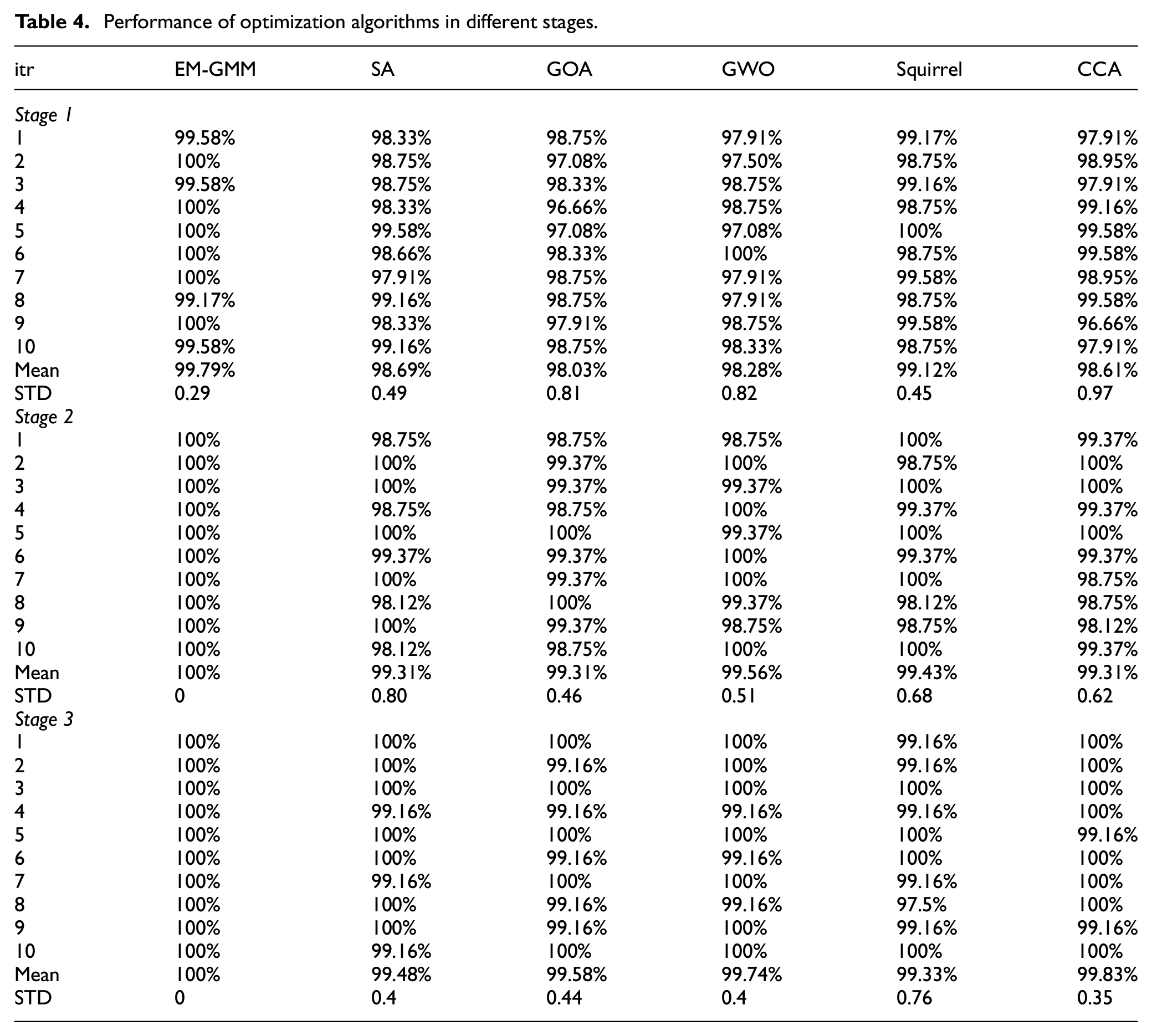
The findings in Table 4 underscore the superiority of the EM-GMM method over other optimization algorithms in terms of accuracy and stability. The achieved accuracy consistently hovers around 100% across all three cases, while the standard deviation (STD) remains nearly zero.

After training the three models, we cascade them as shown in the classification part of the flowchart in Figure 2 to classify the five states of the bearing. While this method has achieved a notable 100% accuracy rate, it’s essential to note that this accuracy becomes significant only when each class has an equal number of samples, which may not always be the case. Consequently, relying solely on this metric may not provide a comprehensive measure of the classifier’s performance.

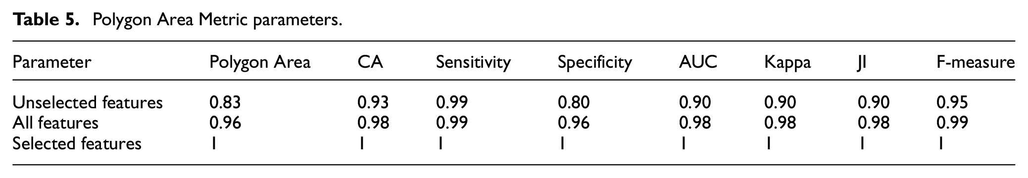
To address this limitation, we introduce the Polygon Area Metric (PAM). ³⁹ Unlike the conventional Classification Accuracy (CA), PAM incorporates five additional metrics, namely Sensitivity (SE), Specificity (SP), Area Under Curve (AUC), Jaccard index (JI), kappa (K), and F-measure (FM). These metrics collectively contribute to a more nuanced evaluation of the classifier’s performance, considering various aspects of its effectiveness. The parameters defining the Polygon Area Metric are as follows:

$$\mathrm{CA}=\frac{\mathrm{TP}+\mathrm{TN}}{\mathrm{TP}+\mathrm{TN}+\mathrm{FP}+\mathrm{FN}}$$

(21)

$$\mathrm{SE}=\frac{\mathrm{TP}}{\mathrm{TP}+\mathrm{FN}}$$

(22)

$$\mathrm{SP}=\frac{\mathrm{TN}}{\mathrm{TN}+\mathrm{FP}}$$

(23)

$$\mathrm{JI}=\frac{\mathrm{TP}}{\mathrm{TP}+\mathrm{FP}+\mathrm{FN}}$$

(24)

$$F=\frac{2\mathrm{TP}}{2\mathrm{TP}+\mathrm{FP}+\mathrm{FP}}$$

(25)

The Polygon Area Metric (PAM) calculates the area of a hexagonal shape formed by points representing the metrics CA, SE, SP, AUC, JI, and FM. This hexagon maintains a regular shape with six sides. For normalization, we divide the area by $2.59807$ , where $2.59807$ denotes the area of a regular hexagon composed of six equilateral triangles, each with a side length of 1.

Table 5 showcases the outcomes of the multi-stage classification procedure, evaluated using the Polygon Area Metric (PAM), across three distinct scenarios: employing all features, utilizing the selected elements, and incorporating the unselected elements. Figure 4 offers a more comprehensive visualization of the results, distinctly demonstrating that the classification utilizing the selected features attains the highest level of performance.

Table 5.

Polygon Area Metric parameters.

Parameter	Polygon Area	CA	Sensitivity	Specificity	AUC	Kappa	JI	F-measure
Unselected features	0.83	0.93	0.99	0.80	0.90	0.90	0.90	0.95
All features	0.96	0.98	0.99	0.96	0.98	0.98	0.98	0.99
Selected features	1	1	1	1	1	1	1	1

Figure 4.

Polygon Area Metric for classification results using: (a) the selected features, (b) using all features, and (c) unselected features.

Conclusion

The imperative nature of bearing fault diagnosis highlights the demand for innovative methodologies, especially in addressing non-stationary conditions. This study introduces a robust multi-stage classification process meticulously designed for identifying combined faults in dynamic, time-varying scenarios, it represents a novel approach to addressing the complexities of bearing fault diagnosis, particularly under variable speed conditions. By breaking down the diagnostic process into stages, we effectively navigate the challenges associated with combined faults and variable operating speeds, providing a more robust and accurate diagnostic solution. We commence our method by decomposing vibration signatures from the “Bearing vibration data collected under time-varying rotational speed conditions” database containing five bearing health states, including a combined fault case to demonstrate the practical applicability of our approach in real-world industrial settings. This validation underscores the effectiveness of our method in addressing the challenges of speed variability and combined fault recognition, which are commonly encountered in machinery operations. We utilize for the signal processing the Empirical Wavelet Transform (EWT) to extract AM-FM modes and derive parameters spanning both time and frequency domains. In the subsequent phase, we employ the Expectation-Maximization Gaussian Mixture Model (EM-GMM) clustering method to select features adept at accurately discerning the precise number of fault classes. Subsequently, we trained classification models for each level utilizing the random forest classifier on the selected features for each stage. A meticulous evaluation employing the Polygon Area Metric (PAM) with six distinct parameters underscores the efficacy of our proposed procedure in adeptly detecting combined defects, even under challenging conditions.

The observed performance increase is due to inheriting several factors in the proposed method. Firstly, we opted for a stage classification approach instead of employing a single classifier for the entire task by utilizing three distinct trained random forest models, each dedicated to a specific stage of the diagnostic process. This division of labor allowed for more focused and specialized processing at each stage, leading to improved performance in fault diagnosis. Furthermore, the selection of features played a crucial role in enhancing the effectiveness of the proposed method. We employed an unsupervised feature selection algorithm to ensure the inclusion of discriminative and informative features. This approach allowed us to identify and prioritize the most relevant features from the input dataset without relying on labeled training data. By focusing on the extraction of robust and representative features, we were able to streamline the diagnostic process and enhance the discriminative power of the classifier ensemble.