Sage Journals: Discover world-class research

Abstract

The radial load distribution integral given by Harris integral method always plays a significant role in calculating the radial load distribution of radial bearings. The error of Harris integral method for calculating the radial load distribution is found caused by the inaccurate values of the radial load distribution integral given by Harris. The radial load distribution integral is corrected in three loading stages using a discrete method. The corrected radial load distribution integral is capable of calculating the load distribution of a bearing with a small load zone caused by a light external load or a great radial clearance. The corrected radial load distribution integral shows different phases varying with the number of rolling elements participating in the radial load transfer. Some specific numerical examples show the higher accuracy and superiority of the corrected radial load distribution integral.

Keywords

Radial bearing radial load distribution discrete calculation method corrected radial load distribution integral small load zone

Introduction

When a radial ball or roller bearing is subjected to a radial load, the load is transferred from one raceway to another through the rolling elements. In this transfer process, the rolling elements are not equally loaded. This uneven load distribution is affected by the amplitude of the external load and the geometry of the rolling bearing¹ and plays a significant role on the operating characteristics of a bearing,² such as the static carrying capacity,^3,4 dynamic vibration,^5–8 radial stiffness,^9–12 and fatigue life.^1,13,14

To determine the radial load distribution, Stribeck¹⁵ first derived an equation to calculate the maximum load on a rolling element of a ball bearing with zero radial clearance. A radial load distribution integral was proposed by Sjövall¹⁶ to calculate the load distribution for nonzero clearances. The integral value is affected by the type of contact in a bearing and the ratio of the radial clearance to the ring radial shift so that the variables of the elliptic integral were introduced into the calculation. This integral is referred to as the Sjövall integral. Based on Sjövall’s research, Harris and Kotzalas¹ proposed a load distribution factor and adjusted the values of the radial load distribution integral by a numerical method which is called Harris integral in this paper. To obtain the integral value more easily, Oswald et al.¹³ and Houpert¹⁷ used different polynomials to fit the relation of integral versus the load distribution factor. A coefficient for the boundary external radial load was defined by Tomović^2,18 to ensure the number of the active rolling elements participating in the external load transfer. Without a calculation of the contact stiffness, Ren et al.¹⁹ proposed a mathematical model in which only the deformations and geometric parameters of the bearing were used to determine the radial load distribution. Moreover, the bearing was considered a mass–spring–damper system, and the load distribution was calculated by multi-body nonlinear dynamic models by Petersen et al.^5,11 and Sawalhi and Randall.^20,21 In addition, a comprehensive explicit dynamic finite element model²² was used to analyze the dynamic contact forces in rotational bearings. Although all the methods are capable of calculating the radial load distribution, most of these methods have specific application conditions. For example, the load zone is assumed to be π and fixed in Stribeck’s¹⁵ equation, which means Stribeck’s method is not suitable for the calculation of the bearings with a nonzero clearance. The discrete models proposed by Tomović^2,18 and Ren et al.¹⁹ cannot be used to obtain the angle scope of the load zone while the dynamic models^11,20 are mostly used for vibration analysis and defect identification. Due to its simplicity, the method based on the load distribution integral has been widely used in many aspects of bearings.^13,17,23,24

However, several open questions remain for calculating the load distribution using the existing integral values. First, in the load distribution result obtained by the values of Sjövall integral or Harris integral, the sum of the vertical components of the calculated rolling element loads is not equal to the external radial load.^1,18,19 This calculation error cannot be neglected if the calculated load is used to predict some critical parameters such as fatigue life.²⁴ Second, when the load distribution factor is greater than 0 and less than 0.1, the value of the Harris integral or the way to calculate the integral are not given in previous studies. It indicates that the current integral method is not applicable for the small load zone situation caused by the light external load or great clearance.¹ The skidding of the rolling elements often occurs and results in smearing type of surface damage under light load situation,²⁵ while the bearing tends to early failure operating with a great clearance.¹³

In this paper, the error of Harris integral method for calculating the radial load distribution in radial bearings is analyzed first. Then, the radial load distribution integral is corrected by using a discrete method. The segmented feature of the corrected load distribution integral is shown. Several numerical examples of commercial bearings are given to illustrate the impact of corrected load distribution integral.

The remainder of the paper is organized as follows. Some necessary initial assumptions for calculating the radial load distribution within radial bearings are listed in Section “Initial assumptions.” The calculation procedure of Harris method and error from Harris integral are introduced and analyzed in Section “Harris method to calculate the radial load distribution.” In Section “Correction of radial load distribution integral,” a discrete method for calculation of load distribution integral is proposed. In Section “Numerical examples and discussion,” the impact of the discrete method is illustrated by several numerical examples of commercial bearings. Finally, the conclusions are presented in Section “Conclusions.”

Initial assumptions

Figure 1 shows the geometries of the radial ball and roller bearings to calculate the radial load distribution. To achieve a practically applicable mathematical model and reduce ambiguous issues, some necessary assumptions should be presented:

(1) Deformation only occurs at the individual contacts between the rolling elements and raceways. It complies with the Hertz elastic contact theory, other parts are absolutely rigid.¹

(2) The bearing is subjected to a static radial load. The dynamic load distribution is considered the same as the static load distribution because, in most applications, the speeds of rotation are almost not as great as to cause ball or roller inertial force of sufficient magnitude to significantly affect the load distribution.¹

(3) An external radial load F_r is downward applied to the inner ring of the bearing, and the outer ring is radially fixed.

(4) For purposes of identifying and locating the position of the rolling elements, the bottom rolling element is set to 0, and the others are numbered clockwise as 1, 2, j, Z−1, where Z is the total number of rolling elements. The rolling element 0 is located in the line of the loading direction of F_r.

(5) The unit azimuth angle β is constant for a bearing with fixed number of rolling elements, which is separated by a cage and calculated by the following formula:

β = \frac{2 π}{Z}

(1)

According to the above assumptions, the load distribution is symmetrical with respect to the line of the loading direction, and the most loaded rolling element is the rolling element 0.

Figure 1.

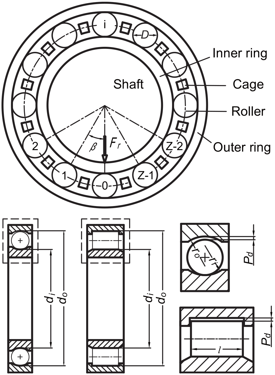
Structure and geometric parameters of the radial ball and roller bearing.

Harris method to calculate the radial load distribution

Harris radial load distribution model and integral

Based on the method proposed by Sjövall,¹⁶ Harris presented a comprehensive model and radial load distribution integral J_r(ε) to calculate the radial load distribution using the load-deflection relationships.¹

For a bearing with rigid support under the radial loads, the radial deflection δ_j of the rolling element at the azimuth location φ_j = jβ is expressed by:

δ_{j} = δ_{r} \cos φ_{j} - \frac{1}{2} P_{d}

(2)

where δ_r is the unknown inner ring radial shift occurring at φ₀ = 0 and P_d is the internal diametral clearance. In terms of maximum deformation δ_max, δ_j can be rearranged as follows:

δ_{j} = δ_{max} [1 - \frac{1}{2 ε} (1 - \cos φ_{j})]

(3)

where

ε = \frac{1}{2} (1 - \frac{P_{d}}{2 δ_{r}})

(4)

ε is defined as the load distribution factor. From equation (4), the angular extent of the half load zone ψ_l is determined by the diametral clearance as follows:

ψ_{l} = \cos^{- 1} (\frac{P_{d}}{2 δ_{r}})

(5)

According to the load-deflection relationship of a rolling element-raceway contact expressed by:

F_{j} = K {δ_{j}}^{n}

(6)

and

\frac{F_{j}}{F_{max}} = {(\frac{δ_{j}}{δ_{max}})}^{n}

(7)

where F_j is the radial load on the rolling element j and F_max is the maximum distributing radial load and is equal to F₀ here. Number n = 3/2 for ball bearings, and n = 10/9 for roller bearings. K is a series of stiffnesses of the inner and outer raceway contact deformation. The calculation of K is illustrated in the Appendix.

From equations (3), (6), and (7), the rolling element load F_j at any rolling element position can be given in terms of the maximum rolling element load F_max by:

F_{j} = F_{max} {[1 - \frac{1}{2 ε} (1 - \cos φ_{j})]}^{n}

(8)

For static equilibrium, the external radial load must equal the sum of the vertical components of the rolling element loads:

F_{r} = \sum_{j = 0}^{j = Z - 1} F_{j} \cos φ_{j}

(9)

F_{r} = F_{max} \sum_{j = 0}^{j = Z - 1} {[1 - \frac{1}{2 ε} (1 - \cos φ_{j})]}^{n} \cos φ_{j}

(10)

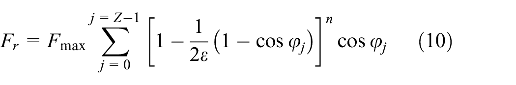
Introducing the radial load distribution integral J_r(ε), equation (10) can be expressed by:

F_{r} = Z F_{max} J_{r} (ε)

(11)

where

J_{r} (ε) = \frac{1}{2 π} \int_{- ψ_{l}}^{+ ψ_{l}} {[1 - \frac{1}{2 ε} (1 - \cos ψ)]}^{n} \cos ψ d ψ

(12)

In Harris’ procedure, the radial integral J_r(ε) has been given numerically for various values of the load distribution factor ε and shown in Table 7.1 and Figure 7.2 in Harris and Kotzalas.¹ From equations (2) and (6), F_max can be expressed as follows:

F_{max} = K δ_{0}^{n} = K {(δ_{r} - \frac{1}{2} P_{d})}^{n}

(13)

Therefore, equation (13) is introduced into equation (11),

F_{r} = ZK {(δ_{r} - \frac{1}{2} P_{d})}^{n} J_{r} (ε)

(14)

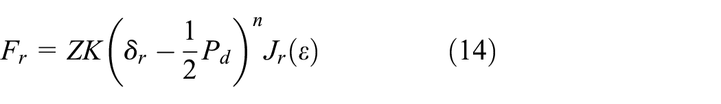
For a given bearing with a given clearance under a given load, δ_r is the only unknown value. Harris and Kotzalas¹ presented that equation (14) may be solved by trial and error. A value of δ_r is first assumed, and ε is calculated from equation (4). Furthermore, the value of J_r(ε) can be yielded from the curves of J_r(ε) versus ε provided by Harris as shown in Table 7.1 and Figure 7.2 in Harris and Kotzalas.¹ If equation (14) does not balance, then the process is repeated. When equation (14) balances, δ_r obtains its value. Then, F_j could be calculated by equations (8) and (13).

Error of Harris model and integral

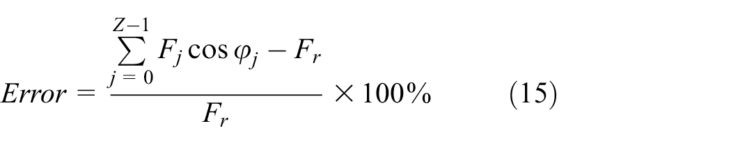
In Harris model mentioned above, three formulas, equations (4), (12), and (14), significantly determine the radial load distribution in a radial bearing. During the calculation using these formulas, as input parameters, the external radial load F_r, total number of rolling elements Z, radial clearance P_d and contact stiffness K do not affect the accuracy of the calculation. However, some calculation errors exist and vary with these input parameters during the calculation of radial load distribution by Harris integral model.^1,18,19 The errors can only be caused by the inaccurate values of J_r(ε) evaluated numerically by Harris. The calculation error is defined as the difference between the sum of the vertical components of distributed load F_j and the external radial load F_r, that is:

E r r o r = \frac{\sum_{j = 0}^{Z - 1} F_{j} \cos φ_{j} - F_{r}}{F_{r}} \times 100 %

(15)

Some examples are given to figure out the influences of Harris integral to the calculation error of Harris method. The values of Harris integral in Table 7.1 and Figure 7.2 from Harris and Kotzalas¹ are used in these examples. When the other input parameters are fixed (F_r = 5000 N, P_d = 0.04 mm, K = 278,630 N/mmⁿ, n = 3/2 for point contact and n = 10/9 for line contact), the errors of Harris method varying with the total number of rolling elements is shown in Figure 2. It is found that the errors of Harris method for both roller and ball bearings become smaller with the increase of the total number of the rolling elements overall, while the values and fluctuation of the error for roller bearing are greater than for ball bearing. The maximum error of these numerical examples is up to nearly 12% when the bearing is a roller bearing with six rollers. Moreover, according to the different number of loaded rolling elements, the errors can be divided into different phases. For example, three rollers participate in the radial load transfer and the error shows a negative-positive-negative trend when Z = 6–12 for the roller bearing. In all of the phases, the variation trends of the errors versus the rolling element number Z are absolutely the same.

Figure 2.

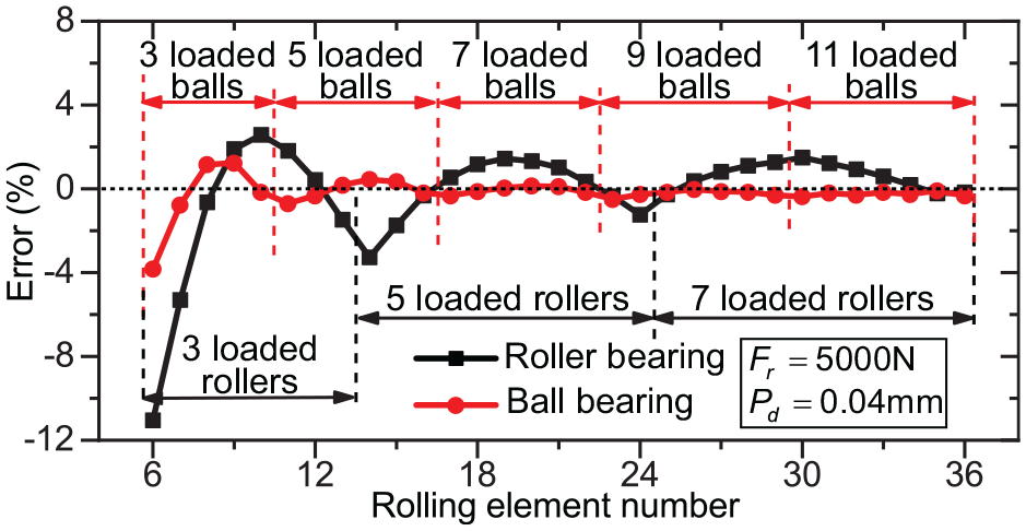
Errors of Harris method versus the total number of rolling elements.

The errors of Harris method under different external radial loads and radial clearances are shown in Figure 3. A roller bearing with 10 rollers and K = 278,630 N/mm^10/9 is chosen in these examples. The error of Harris method is considered to raise with the growth of F_r by Ren et al.¹⁹ However, some different trends are indicated in Figure 3. According to different load zone extents, the load distribution in a radial bearing with 10 rollers is divided into six phases as shown in Figure 4. Phase I–VI, respectively corresponding to only one rolling element participating in load transfer to all rolling elements participating in load transfer, introduce the evolution of the load distribution with the load distribution factor ε. These phases are marked in Figure 3. As shown in Figure 3(a), overall, a bigger radial clearance indicates a severer error when P_d > 0, and the error decreases with the increase of the external radial load. The maximum error with a value of about 17.5% appears when there are the maximum P_d and minimum F_r. Differing from the case of positive clearance, the maximum values of Harris method error are no more than 1% and hardly affected by the values of the clearance when P_d < 0 as shown in Figure 3(b). For different radial clearances, although the scopes of the same load phase are different, the variation and values of the error varying with F_r are almost the same in the same load phase. For example, in Figure 3(a), the error shows a negative-positive-negative trend varying with F_r in all of the phase II, while the error tends to vary from negative values to zero in all of the phase III. In Figure 3(b), the errors in all phase VI are absolutely zero, and the error shows a positive-negative-positive trend in all of the phase IV, while the error decreases with the increase of F_r in all of the phase III. It is indicated that the error of Harris method is significantly affected by the load zone extent, that is, the load distribution factor ε.

Figure 3.

Errors of Harris method versus the external radial loads and radial clearances: (a) positive clearances and (b) negative clearances.

Figure 4.

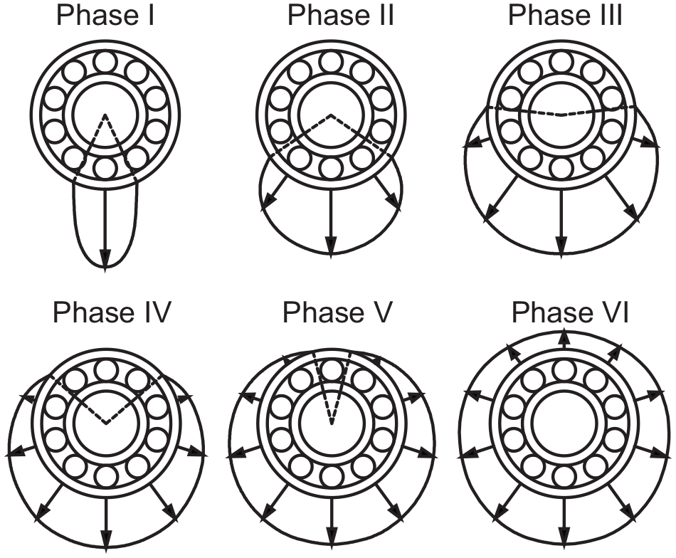
Six load phases of the radial bearing with 10 rolling elements.

With the load distribution factor ε as the independent variable and the error as the dependent variable, Figure 5 shows the error varying with ε for a roller bearing with 10 rollers. Different load phases are marked in Figure 5. It is shown that the error varies with ε following different trends in different load phases when ε < 1 and almost keeps a values of zero when ε > 1. Moreover, the smaller the load distribution factor ε is, the severer the variation scope and the maximum value of the errors are. Because the input parameters do not affect the accuracy of the calculation, all of the errors are absolutely caused by the inaccurate values of J_r(ε) evaluated numerically by Harris. Besides, when 0 < ε < 0.1, the values of J_r(ε) is not given by Harris, which implies Harris integral method does not apply to the situation of a small load zone of ψ_l < 36.87° (calculated by equation (4) and (5) when ε < 0.1) caused by a light external load or a great radial clearance. So, it is necessary to correct J_r(ε) for calculating the load distribution of radial bearings accurately by integral method.

Figure 5.

Error of Harris method versus the load distribution factor for a roller bearing with 10 rollers.

Correction of radial load distribution integral

Calculation of load distribution integral by discrete method

A discrete method is proposed to correct the radial load distribution integral here. The equilibrium between the external radial load and the sum of the vertical components of the rolling element loads can be expressed in two forms: discrete form as equation (10) and integral form as equation (11). Comparing these two formulas, the radial load distribution integral can be expressed by discrete form:

J_{r} (ε) = \frac{1}{Z} \sum_{j = 0}^{j = Z - 1} {[1 - \frac{1}{2 ε} (1 - \cos φ_{j})]}^{n} \cos φ_{j}

(16)

However, because of the upper and lower limits of the summation in equation (16), this formula is only suitable for the case of ε > 1, that is, the situation of all of the rolling elements participating in the load transfer. To calculate the values of J_r(ε) when ε < 1, the number of active rolling elements need to be ensured, and the upper and lower limits of the summation in equation (16) need to be adjusted. When ε < 1, it is assumed that the rolling element at the two ends of the load zone are numbered k and Z−k. Thus, in the load zone, the number of rolling elements participating in the load transfer is 2k + 1 and j = 0, 1, Z−1, 2, Z−2, …, k, Z−k. The integral J_r(ε) for ε < 1 can be expressed as:

\begin{matrix} J_{r} (ε) = \frac{1}{Z} {\sum_{j = 0}^{k} {[1 - \frac{1}{2 ε} (1 - \cos φ_{j})]}^{n} \cos φ_{j} \\ + \sum_{j = Z - k}^{Z - 1} {[1 - \frac{1}{2 ε} (1 - \cos φ_{j})]}^{n} \cos φ_{j}} \end{matrix}

(17)

As long as the value of k is ensured, the value of J_r(ε) can be calculated by equation (17). From equations (4) and (5), the relationship between the angular extent of the half load zone ψ_l and the load distribution factor ε can be expressed as follows:

ψ_{l} = \cos^{- 1} (1 - 2 ε)

(18)

Furthermore, because the angle between two adjacent rollers is the unit azimuth angle β, the value of k depends on how many β are contained in ψ_l:

k = ⌊ \frac{ψ_{l}}{β} ⌋ = ⌊ \frac{\cos^{- 1} (1 - 2 ε)}{β} ⌋

(19)

When ψ_l < β, that is, ε < (1−cosβ)/2, there is only one rolling element participating in the load transfer and k = 0. Introducing k = 0 into equation (17), the values of J_r(ε) when only one rolling element participates in the load transfer can be calculated as follows:

J_{r} (ε) = \frac{1}{Z}

(20)

When ψ_l > β, that is, ε > (1−cosβ)/2, according to the initial assumptions in this paper, the load distribution is symmetrical with respect to the line of loading direction. Thus,

\cos φ_{k} = \cos φ_{Z - k}

(21)

Then, equation (17) can be simplified as:

J_{r} (ε) = \frac{1}{Z} {1 + 2 \sum_{j = 1}^{k} {[1 - \frac{1}{2 ε} (1 - \cos φ_{j})]}^{n} \cos φ_{j}}

(22)

In summary, J_r(ε) can be computed from equation (23):

J_{r} (ε) = \frac{1}{Z}, 0 < ε < (1 - \cos \frac{2 π}{Z}) / 2

(23a)

\begin{matrix} J_{r} (ε) = \frac{1}{Z} {1 + 2 \sum_{j = 1}^{k} {[1 - \frac{1}{2 ε} (1 - \cos φ_{j})]}^{n} \cos φ_{j}}, \\ (1 - \cos \frac{2 π}{Z}) / 2 \leq ε < 1 \end{matrix}

(23b)

J_{r} (ε) = \frac{1}{Z} \sum_{j = 0}^{j = Z - 1} {[1 - \frac{1}{2 ε} (1 - \cos φ_{j})]}^{n} \cos φ_{j}, ε \geq 1

(23c)

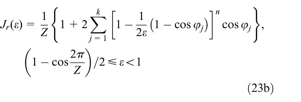
Equation (23) shows that J_r(ε) is actually affected by the number of rolling elements. For a given bearing, Z and n are fixed, and a value of ε corresponds to a value of J_r(ε) for ε > 0. To obtain the curve of J_r(ε) varying with ε, ε is considered the independent variable with an initial value and increment of both 0.0001 and no more than the constant C. The constant C is defined as the maximum value of ε during the calculation of J_r(ε). A judgement is needed that if there is only one loaded rolling element. If only one rolling element is loaded, then J_r(ε) is equal to 1/Z. With the increase of ε, when there is more than one rolling element taking part in the transfer of F_r, J_r(ε) can be calculated by equations (23b) or (23c). The parameter k in equation (23b) is first assumed to be 1. When (1−cosβ)/2 ≤ ε < 1, if ψ_l is less than 2β, there are three rolling elements loaded. If ψ_l is no less than 2β, k is added to 2, and the process mentioned above is repeated. The solving procedure to calculate J_r(ε) is expressed in a flowchart shown in Figure 6.

Figure 6.

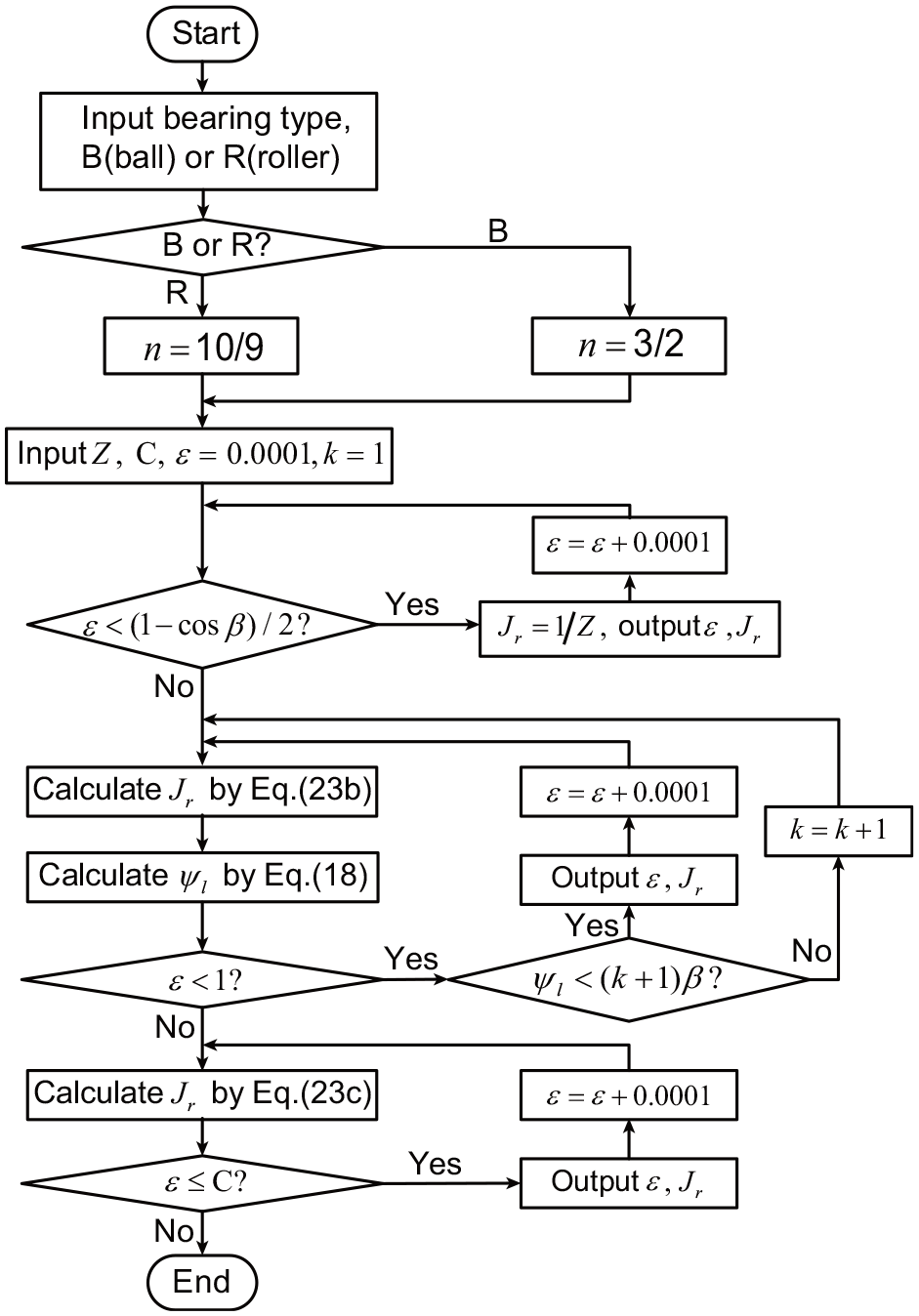
Calculation flowchart of the radial load distribution integral by the discrete method.

Examples for the corrected radial load distribution integral

Figure 7 shows the curves of the corrected radial load distribution integral varying with ε. Eight values of the number of rolling elements Z are considered as examples. The black and red points are the values of Harris integral.¹ It is found that when ε < 1, that is, the angular extent of the load zone is less than 360°, the corrected radial load distribution integral differs from Harris integral and actually varies with the number of rolling elements, while the corrected integral is almost the same with Harris integral and not affected by the number of rolling elements when ε > 1, that is, all the rolling elements in a bearing participate in the radial load transfer. Furthermore, as shown in the enlarged view (a) in Figure 7, the corrected curves introduce the values of J_r(ε) corresponding to 0 < ε < 0.1, which cannot be given by Harris integral. It denotes that the corrected radial load distribution integral makes it possible to calculate the load distribution of a bearing with a small load zone (less than 73.74°). Besides, as shown in the enlarged view (b) in Figure 7, it is suggested that the effect of the number of rolling elements on the integral J_r(ε) is severer for line contact than point contact when ε < 1, which explains why the values and fluctuation of the error for roller bearing are greater than for ball bearing in Figure 2.

Figure 7.

Corrected radial load distribution integral of different number of rolling elements: (a) Corrected integral for a wide range of load distribution factor, (b) enlarged view of the corrected integral.

In order to illustrate the trend of the corrected radial load distribution integral varying with the scope of the load zone, the corrected curve of line contact and Z = 10 is chosen as an example and shown in Figure 8(a). The black curve is the corrected integral while the red curve is Harris integral for line contact in Figure 8(a). It is shown that some obvious turning points exist in the corrected curve corresponding to some specific load distribution factor ε. According to the calculation flow of the corrected J_r(ε), every time the value of k increases, a turning point appears in the curves of the corrected J_r(ε). These turning points divide the corrected curve into six load phases, phases I–VI. These phases exactly correspond to the six load phases shown in Figure 4. As shown in Figure 8(a), the corrected J_r(ε) remains the value of 0.1 in phase I where Harris integral curve fails to give the value of J_r(ε). In phases II–V, the corrected integral curve and Harris integral curve do not coincide at most values of ε except for some intersections, while these two curves almost absolutely coincide in phases VI. Figure 8(b) shows the difference between the corrected radial load distribution integral and Harris integral which represents the degree of correction to Harris integral. It is found that the variation trend of the difference ΔJ_r(ε) versus ε in Figure 8(b) is absolutely the same with that of the error caused by Harris integral versus ε in Figure 5. Moreover, comparing the values of the difference ΔJ_r(ε) and the error caused by Harris integral, it is shown that, for a roller bearing with 10 rollers, a deviation of about 0.02 in radial load distribution integral can cause a calculation error of nearly 20%, which suggests the accuracy of the radial load distribution integral is significant for calculating the load distribution accurately.

Figure 8.

Corrected radial load distribution integral and Harris integral for a radial roller bearing with 10 rollers: (a) comparison and (b) difference.

To illustrate the influence of the rolling element number to the radial load distribution integral when ε < 1, the corrected J_r(ε) curves of Z = 10–17 are shown in Figure 9(a) to (h) respectively. The number of the load phases increase from five for Z = 10 to nine for Z = 17 in Figure 9. It is demonstrated that the number of the turning points as well as the load phases increase with the increase of Z, and is equal to ⌈Z/2⌉. This effect of the rolling element number on the divided phases is caused by the variation of the unit azimuth angle β calculated by equation (1). As shown in equation (1), the unit azimuth angle β decreases with the increase of Z. Then according to equation (23a), the scope of phase I of J_r(ε) becomes narrower with the increase of Z. Furthermore, when (1−cosβ)/2 ≤ ε < 1, for a fixed value of ε, that is, a fixed scope of load zone, more rolling elements participate in the load transfer with the decrease of β. It manifests that, with the increase of the number of rolling elements, the same load phase tends to be narrower and move toward smaller values of ε, and new load phases with more active rolling elements appear. Therefore, the number of the load phases increases with the increase of Z. Moreover, although the same load phase tends to be narrower with the increase of Z, for a fixed number of rolling element, different phases correspond to a same angle range of 2β except for the last load phase. As shown in Figure 10, according to the assumption 4, there is a rolling element between two adjacent unit azimuth angles located at the top of a radial bearing with even numbers of rolling element, while there is a unit azimuth angle between two adjacent rolling elements located at the top of a radial bearing with odd numbers of rolling element. Therefore, the angle range of the last load phases in Figure 9(a) to (h) is equal to 2β for even numbers of rolling element and equal to β for odd numbers of rolling element.

Figure 9.

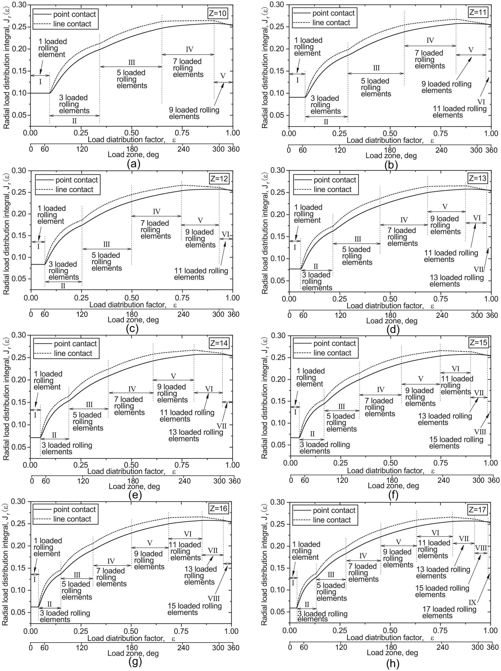
Corrected radial load distribution integral for point and line contact with 10–17 rolling elements corresponding to (a)–(h).

Figure 10.

Schematic view of the radial bearing with (a) even number of rolling elements and (b) odd number of rolling elements.

According to the statements above, there are some characteristics of the corrected integral:

(1) The corrected radial load distribution integral makes it possible to calculate the load distribution of a bearing with a small load zone with 2ψ_l < 73.74° caused by a light external load or a great radial clearance.

(2) The corrected radial load distribution integral is determined by the load distribution factor, the azimuth location further the total number of rolling element in a radial bearing.

(3) For a bearing with a given number of rolling element, the corrected radial load distribution integral shown in Figure 9 can be used to intuitively ensure the number of rolling element participating in the load transfer and the extent of the load zone.

Numerical examples and discussion

Some specific numerical examples for the calculation of the radial load distribution are given to illustrate the performance of the proposed correction of the radial load distribution integral. The conditions of the radial load distribution in these examples cover both radial ball and roller bearings with positive and negative clearances under different loads. Moreover, the results of the calculation by the corrected radial load distribution integral are compared with those calculated by Harris integral to show the improvement of the calculation accuracy.

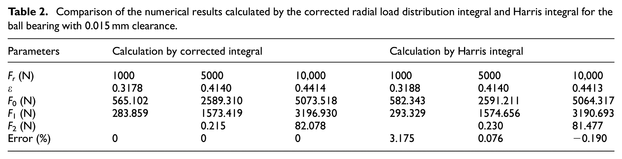
A single row deep groove ball bearing 6209 with odd number of rolling elements and a single row cylindrical roller bearing NU209 with even number of rolling elements are considered in the numerical examples. The parameters of the ball and roller bearings for the numerical calculation are shown in Table 1. The radial clearances shown in Table 1 are the initial clearance chosen from the Rolling Bearing Catalogue of SKF.²⁶ An interference fitting clearance of −0.010 mm is chosen as the negative clearance for both ball and roller bearings in the numerical examples. Three values of the external radial load F_r are introduced to the calculation. According to these parameters in Table 1, the numerical results of the ball and roller bearings calculated by the corrected J_r(ε) and Harris J_r(ε) are displayed in Tables 2 to 5, respectively. The error of the results here is defined as equation (15).

Table 1.

Parameters of ball bearings 6209 and roller bearing NU209^1,26 for the numerical examples.

Ball bearing 6209	P_d (mm)	0.015
	Z	9
	D (mm)	12.700
	d_i (mm)	52.292
	d_o (mm)	77.706
	r_i (mm)	6.600
	r_o (mm)	6.600
Roller bearing NU209	P_d (mm)	0.040
	Z	14
	l (mm)	9.601

Table 2.

Comparison of the numerical results calculated by the corrected radial load distribution integral and Harris integral for the ball bearing with 0.015 mm clearance.

Parameters	Calculation by corrected integral			Calculation by Harris integral
F_r (N)	1000	5000	10,000	1000	5000	10,000
ε	0.3178	0.4140	0.4414	0.3188	0.4140	0.4413
F ₀ (N)	565.102	2589.310	5073.518	582.343	2591.211	5064.317
F ₁ (N)	283.859	1573.419	3196.930	293.329	1574.656	3190.693
F ₂ (N)		0.215	82.078		0.230	81.477
Error (%)	0	0	0	3.175	0.076	−0.190

Table 3.

Comparison of the numerical results calculated by the corrected radial load distribution integral and Harris integral for the ball bearing with −0.010 mm clearance.

Parameters	Calculation by corrected integral			Calculation by Harris integral
F_r (N)	1000	5000	10,000	1000	5000	10,000
ε	0.9204	0.5876	0.5511	0.9213	0.5878	0.5512
F ₀ (N)	432.585	2320.970	4728.940	431.835	2311.925	4710.094
F ₁ (N)	352.798	1663.600	3306.271	352.258	1657.352	3293.319
F ₂ (N)	176.981	375.306	592.111	176.877	374.3567	590.199
F ₃ (N)	34.469			34.622
Error (%)	0	0	0	−0.167	−0.377	−0.393

Table 4.

Comparison of the numerical results calculated by the corrected radial load distribution integral and Harris integral for the roller bearing with 0.040 mm clearance.

Parameters	Calculation by corrected integral			Calculation by Harris integral
F_r (N)	1000	5000	10,000	1000	5000	10,000
ε	0.0832	0.1932	0.2533	—	0.1904	0.2551
F ₀ (N)	602.323	2157.290	3716.601	—	2104.554	3786.782
F ₁ (N)	220.639	1552.340	2918.810	—	1505.991	2979.454
F ₂ (N)		36.408	821.021	—	14.402	855.069
Error (%)	0	0	0	—	−3.276	−2.118

Table 5.

Comparison of the numerical results calculated by the corrected radial load distribution integral and Harris integral for the roller bearing with −0.010 mm clearance.

Parameters	Calculation by corrected integral			Calculation by Harris integral
F_r (N)	1000	5000	10,000	1000	5000	10,000
ε	3.506	1.095	0.739	3.506	1.095	0.741
F ₀ (N)	917.431	1522.860	2703.460	916.927	1522.977	2694.401
F ₁ (N)	903.046	1446.533	2503.171	902.549	1446.670	2495.107
F ₂ (N)	862.863	1234.861	1950.810	862.387	1235.000	1945.472
F ₃ (N)	805.128	935.456	1180.900	804.683	935.597	1179.300
F ₄ (N)	741.531	614.291	386.704	741.118	614.432	388.717
F ₅ (N)	684.694	388.872		684.311	339.011
F ₆ (N)	645.633	160.368		645.271	160.501
F ₇ (N)	631.749	100.575		631.394	100.703
Error (%)	0	0	0	−0.052	0.002	−0.318

It is shown that the errors of the results calculated by the corrected J_r(ε) are all nil, while the errors of the results calculated by Harris J_r(ε) are obvious and vary with ε following the rules illustrated in Section “Harris method to calculate the radial load distribution.” It is indicated that the corrected J_r(ε) can be used to obtain a more accurate radial load distribution than the value of J_r(ε) given by Harris shown in Figure 7.2 in Harris and Kotzalas.¹ Moreover, as shown in Table 4, when P_d = 0.040 mm and F_r = 1000 N, the calculation by the corrected radial load distribution integral shows an accurate solution, while the calculation by Harris integral failed to obtain the load distribution due to the defect of the values of Harris J_r(ε) when 0 < ε < 0.1.

Under the situation of a small load zone caused by a light external load or a great radial clearance, the load distribution plays a significant role in the studies of skidding behavior^25,27 and the fatigue life¹³ of bearings. The sliding velocities of the rollers are considered to exist under light external loads and vary with the radial load distribution in the bearing by Tu et al.²⁵ and Han et al.²⁷ Moreover, the skidding of the roller at the entry of the loaded zone is likely to cause wear on the raceway surface.²⁵ Thus, accurate calculation of the load distribution under light load condition can be used to ensure the skidding states of the rollers and the locations of the possible wear. Furthermore, a greater radial clearance will cause a kind of load distribution with a smaller load zone and a greater maximum rolling element load. Then, the fatigue life of the bearing will decrease under this kind of load distribution.¹³ Therefore, accurate calculation of the load distribution under great clearance condition contributes to avoiding early failure caused by improper assembly. Besides, according to the calculation method of fatigue life proposed by Lundberg and Palmgren,²⁴ the basic dynamic capacity of a bearing is calculated by the radial load distribution and the radial load distribution integral. It reveals that the errors of radial load distribution and radial load distribution integral will be transferred and accumulated in the calculation of the fatigue life of bearings. Thus, the correction of the radial load distribution integral and its contribution on the accurate calculation of the load distribution are significant for predicting the fatigue life accurately especially for the light load or great clearance conditions.

Conclusions

In this paper, the error from Harris method to calculate the radial load distribution in radial bearings was analyzed. A discrete method was proposed to correct the radial load distribution integral for radial bearings. The calculation of the corrected J_r(ε) was divided into three stages according to the values of the load distribution factor ε. Some numerical examples were used to illustrate the characteristics and application of the corrected radial load distribution integral. The following conclusions were obtained:

(1) The errors of Harris method are affected by the load distribution factor ε and absolutely caused by the inaccurate values of the radial load distribution integral evaluated numerically by Harris.

(2) The corrected radial load distribution integral is effective for calculating the load distribution under the situation of a small load zone caused by a light external load or a great radial clearance (0 < ε < 0.1), which cannot be solved by Harris integral. Under this small load zone situation, the corrected radial load distribution integral contributes to ensuring the bearing skidding states and avoiding early failure caused by improper assembly.

(3) The corrected radial load distribution integral shows the effect of the rolling element number on the values of J_r(ε) when the load distribution factor ε is less than 1, that is, not all rolling elements participate in the load transfer.

(4) For a given number of rolling elements, the corrected curves of J_r(ε) versus ε can be divided into some load phases according to the number of rolling elements and used to intuitively ensure the radial load distribution in the bearing.

(5) The accuracy of the integral method to calculate the radial load distribution is improved by the corrected radial load distribution integral, which are significant for predicting the fatigue life more accurately according to the theory of Lundberg-Palmgren.

Footnotes

Appendix

Handling Editor: Associate Professor Michal Hajžman

Declaration of conflicting interests

The author(s) declared no potential conflicts of interest with respect to the research, authorship, and/or publication of this article.

Funding

The author(s) disclosed receipt of the following financial support for the research, authorship, and/or publication of this article: This work supported by the National Natural Science Foundation of China (Grant No. 12302238), and the National Key Research and Development Program of China (Grant No. 2021YFB3400701).

ORCID iD

Xi Wang

References

Harris

Kotzalas

MN.

Rolling bearing analysis: essential concepts of bearing technology. 5th ed. Boca Raton, FL: Taylor & Francis, 2007.

Tomovic

Investigation of the effect of rolling bearing construction on internal load distribution and the number of active rolling elements. Adv Mater Res 2013; 633: 103–116.

Glodež

Potočnik

Flašker

Computational model for calculation of static capacity and lifetime of large slewing bearing’s raceway. Mech Mach Theory 2012; 47: 16–30.

Potočnik

Göncz

Glodež

Static capacity of a large double row slewing ball bearing with predefined irregular geometry. Mech Mach Theory 2013; 64: 67–79.

Petersen

Howard

Prime

Varying stiffness and load distributions in defective ball bearings: analytical formulation and application to defect size estimation. J Sound Vib 2015; 337: 284–300.

Brie

Modelling of the spalled rolling element bearing vibration signal: an overview and some new results. Mech Syst Signal Process 2000; 14: 353–369.

Zhang

Han

Peng

, et al. A comprehensive dynamic model to investigate the stability problems of the rotor-bearing system due to multiple excitations. Mech Syst Signal Process 2016; 70–71: 1171–1192.

Wang

Han

, et al. Contact trajectory of angular contact ball bearings under dynamic operating condition. Tribol Int 2016; 104: 247–262.

Hernot

Sartor

Guillot

Calculation of the stiffness matrix of angular contact ball bearings by using the analytical approach. J Mech Des Trans ASME 2000; 122: 83–90.

10.

Liu

Tang

, et al. An analytical calculation method of the load distribution and stiffness of an angular contact ball bearing. Mech Mach Theory 2019; 142: 103597.

11.

Petersen

Howard

Sawalhi

, et al. Analysis of bearing stiffness variations, contact forces and vibrations in radially loaded double row rolling element bearings with raceway defects. Mech Syst Signal Process 2015; 50–51: 139–160.

12.

Szumiński

Determination of the stiffness of rolling kinematic pairs of manipulators. Mech Mach Theory 2007; 42: 1082–1102.

13.

Oswald

Zaretsky

Poplawski

J V.

Effect of internal clearance on load distribution and life of radially loaded ball and roller bearings. Tribol Trans 2012; 55: 245–265.

14.

Nagatomo

Takahashi

Okamura

, et al. Effects of load distribution on life of radial roller bearings. J Tribol 2012; 134: 1–7.

15.

Stribeck

Ball bearings for various loads. Trans ASME 1907; 29: 420–463.

16.

Sjövall

The load distribution within ball and roller bearings under given external radial and axial load. Tek Tidskr Mek 1933; 9: h9.

17.

Houpert

. A uniform analytical approach for ball and roller bearings calculations. J Tribol 1997; 119: 851–858.

18.

Tomović

Calculation of the necessary level of external radial load for inner ring support on q rolling elements in a radial bearing with internal radial clearance. Int J Mech Sci 2012; 60: 23–33.

19.

Ren

Zhai

Ren

Calculation of radial load distribution on ball and roller bearings with positive, negative and zero clearance. Int J Mech Sci 2017; 131–132: 1–7.

20.

Sawalhi

Randall

. Simulating gear and bearing interactions in the presence of faults. Part I. The combined gear bearing dynamic model and the simulation of localised bearing faults. Mech Syst Signal Process 2008; 22: 1924–1951.

21.

Sawalhi

Randall

RB.

Simulating gear and bearing interactions in the presence of faults. Part II: simulation of the vibrations produced by extended bearing faults. Mech Syst Signal Process 2008; 22: 1952–1966.

22.

Singh

Köpke

Howard

, et al. Analyses of contact forces and vibration response for a defective rolling element bearing using an explicit dynamics finite element model. J Sound Vib 2014; 333: 5356–5377.

23.

Palmgren

Ball and roller bearing engineering. 3rd ed. Philadelphia, PA: Burbank Philadelphia, 1959.

24.

Lundberg

Palmgren

Dynamic capacity of rolling bearings. Acta Polytech Scand Mech Eng Ser 1947; 1: 5–58.

25.

Luo

Investigation of the dynamic local skidding behaviour of rollers in cylindrical roller bearings. Proc Inst Mech Eng Part K J Multi-Body Dyn 2019; 233: 899–909.

26.

SKF. Rolling bearings catalogue 17000 EN. Pune: SKF Group, 2018.

27.

Han

Chu

Skidding behavior of cylindrical roller bearings under time-variable load conditions. Int J Mech Sci 2018; 135: 203–214.

28.

Brewe

Hamrock

BJ.

Simplified solution for elliptical-contact deformation between two elastic solids. J Tribol 1977; 99: 485–487.

A discrete calculation method for radial load distribution integral of radial bearings

Abstract

Keywords

Introduction

Initial assumptions

Harris method to calculate the radial load distribution

Harris radial load distribution model and integral

Error of Harris model and integral

Correction of radial load distribution integral

Calculation of load distribution integral by discrete method

Examples for the corrected radial load distribution integral

Numerical examples and discussion

Conclusions

Footnotes

Appendix

Declaration of conflicting interests

Funding

ORCID iD

References