Sage Journals: Discover world-class research

Abstract

Low-frequency noise caused by structural vibration has a significant impact on the comfort of wheel loader drivers. To reduce the adverse effects of vibration noise on drivers and improve their comfort, this study proposes a low-noise structural optimization method based on an approximate model. To accurately obtain the vibration noise data of the wheel loader’s driver cab, a designed experiment was conducted to collect vibration and internal noise data under specific working conditions. The frequency response method and panel acoustic contribution analysis method were used to analyze the structural vibration characteristics and acoustic response characteristics of the driver cab, respectively. The panels that have a significant impact on the vibration noise of the driver cab were identified, and their thicknesses were defined as design variables to establish an optimization model. Meanwhile, a response surface method was used to construct an approximate model, and the NSGA-II algorithm (Non-dominated Sorting Genetic Algorithm-II) was used to solve the optimization model and obtain the optimized driver cab structure. The results show that the maximum noise peak (117 Hz) of the loader cab was successfully reduced by 2.9 dB after optimization. This result demonstrates the effectiveness and feasibility of the proposed method.

Keywords

Wheel loader panel acoustic contribution analysis response surface method approximation model

Introduction

With the gradual development of construction machinery, people’s requirements for comfort have been continuously improving in recent years. Noise not only reduces passenger comfort but also has an impact on their physical and mental health.¹ In recent years, there has been research on the noise generation mechanisms and noise reduction measures for various types of transportation, such as analysis of noise transmission paths² and the study of sound-absorbing materials.³ The wheel loader is a typical engineering machinery vehicle, and the interior noise in the passenger compartment is one of the main components that affects comfort. From the perspective of the causes of noise, the interior noise of the cab includes structure-borne noise and air-borne noise. Air-borne noise refers to the noise that external sound sources directly enter the cab through the air, and structure-borne noise is formed due to vibrations in the cab panels caused by external excitations. The noise caused by structural vibration typically falls within the mid-to-low frequency range, with 20–200 Hz being a notable range of interest. The noise in this frequency range is mainly due to the radiated noise caused by the vibration of the cabin wall panels.^4,5

Some studies are based on the dynamic response of the cab structure and the structure-acoustic coupling calculation method to analyze and predict the interior noise of the cab. At the same time, a systematic approach called Panel Acoustic Contribution Analysis (PACA) is widely used in structure-borne noise research, which has guiding significance for the design of low-noise structures in cabs.^6,7 In general, the purpose of these methods is to reduce the vibration amplitude of the cab panels and improve the acoustic environment inside the cab. Jiao et al.⁸ combined the finite element method (FEA) with statistical energy analysis (SEA) to establish a FE-SEA hybrid model for predicting low-frequency structure-borne noise in the cab. In order to reduce the impact of low-frequency noise on passenger comfort during subway operation, Zhang et al.⁹ predicted and calculated the low-frequency noise in the subway by the finite element method, and used the plate contribution analysis to obtain the key areas for generating low-frequency noise, and used the method of paving damping materials to make the maximum sound pressure level decrease by 7.8 dB. Guo et al.¹⁰ used the finite element method to calculate the structural characteristics of the body-in-white and the body panel velocity. They then achieved the interior acoustic response and panels acoustic contribution analysis (PACA). Finally, they adopted con-strained damping treatments to control the panel vibration based on the PACA results, which resulted in a reduction of 2.0 dB at 54 Hz and 7.4 dB at 135 Hz. Han et al.⁵ introduced the parameters of “total sound contribution” and “total sound field contribution” into PACA and used their established auto finite element modal analysis to evaluate the comprehensive sound contribution of auto body panels. They then added a damping layer to the body panel area, resulting in a reduction of nearly or over 15 dB in the total sound pressure levels at the field points. In a similar vein, Liu et al.¹¹ proposed a composite panel acoustic contribution analysis method considering multi-frequency for the shortcomings of the traditional panel acoustic contribution analysis that does not consider single-frequency contribution, which integrates the results of the panel contribution and the modal contribution to identify the panels and regions that need to be optimized. Using this method, they successfully reduced the low-frequency noise of the excavator cab by 2.25 dB.

Based on the aforementioned studies, analyzing the acoustic characteristics of the cab interior typically involves using the vibration response of the cab panel as a boundary condition for further investigation. The vibration response results are usually obtained through testing or calculating a finite element model.

In addition, the results of Panel Acoustic Contribution Analysis for cab often consist of multiple panels that need to be optimized, rather than just a single panel. For problems with multiple design variables like this, it is necessary to establish mathematical models and select appropriate optimization methods for calculation. However, the construction of these mathematical models requires repeatedly solving structure-acoustic finite element models, which poses a significant challenge to the computer performance and solution time. Therefore, an approximate model is introduced into the optimization process. Approximate models are a common method used to reduce calculation costs and improve efficiency,¹² and they have been widely applied in other fields of the finite element calculations.^13–15

This study proposes an optimization method based on an approximate model for reducing low-frequency structure-borne noise in loader cabs. After verifying the accuracy of the established finite element model through experiments, the study uses the Panels Acoustic Contribution Analysis method to analyze the key components that have a significant impact on the sound pressure near the ear. Based on the analysis results, an optimization model is constructed to optimize the thickness of the panels in the loader cab, and relevant conclusions are drawn.

Basic theory

Frequency response theory

The frequency response analysis is a function with frequency as the independent variable, describing the Fourier transform relationship between response and excitation. It is an inherent characteristic of the structure, independent of the magnitude of the load, and is only related to the stiffness, mass, and damping characteristics of the structure. The motion equation of a multi-degree-of-freedom system under harmonic excitation is expressed as equation (1).¹⁶

[M] {\overset{\cdot\cdot}{x} (t)} + [C] {\overset{\cdot}{x} (t)} + [K] {x (t)} = {f (w)} e^{iwt}

(1)

In equation (1), [M], [C], and [K] represent the mass, damping, and stiffness matrices of the system, respectively. {x(t)} is the displacement response vector at each point in the system, and ${f (w)} e^{iwt}$ represents the external excitation, where w is the excitation frequency.

Introducing the assumed solution is represented by equation (2).

{x} = [φ] {ε (w)} e^{i ω t}

(2)

During the process of introducing assumed solutions, the physical coordinates have been transformed into modal coordinates using the modal matrix {ε(w)}.

The equation obtained by substituting the form equation (2) into equation (1) and ignoring damping is as follows:

- w^{2} [M] [φ] {ξ (w)} + [K] [φ] {ξ (w)} = {f (w)}

(3)

Equation (3) is still coupled, and multiplying by [φ]^T in front gives equation (4).

- w^{2} {[φ]}^{T} [M] [φ] {ξ (w)} + {[φ]}^{T} [K] [φ] {ξ (w)} = {[φ]}^{T} {f (w)}

(4)

By utilizing the orthogonal properties of matrices, the motion equations are expressed using the generalized mass matrix and the generalized stiffness matrix to improve the speed of solving the equation system.

The structural displacement or sound pressure is obtained by linearly combining various vibration modes or sound modes, and it is transformed into modal space through the equation (5).

{\begin{matrix} u = ϕ_{s} ξ_{s} \\ u = ϕ_{f} ξ_{f} \end{matrix}

(5)

In equation (5), $ϕ_{s}$ represents the non-coupled undamped structural mode, $ϕ_{f}$ represents the non-coupled undamped rigid boundary acoustic mode, $ξ_{s}$ and $ξ_{f}$ represent the modal participation factors.

The matrix equation in modal form is obtained by multiplying the left side by the transpose of the modal matrix.

\begin{matrix} (\begin{matrix} M_{s} & 0 \\ M & M_{f} \end{matrix}) (\begin{matrix} {\overset{\cdot\cdot}{ξ}}_{s} \\ {\overset{\cdot\cdot}{ξ}}_{f} \end{matrix}) + (\begin{matrix} C_{s} & 0 \\ 0 & C_{f} \end{matrix}) (\begin{matrix} {\overset{\cdot}{ξ}}_{s} \\ {\overset{\cdot}{ξ}}_{f} \end{matrix}) \\ + (\begin{matrix} K_{s} & - K \\ 0 & K_{f} \end{matrix}) (\begin{matrix} ξ_{s} \\ ξ_{f} \end{matrix}) = (\begin{matrix} Q_{s} \\ 0 \end{matrix}) \end{matrix}

(6)

In equation (6), $M_{s} = ϕ_{s}^{T} m_{s} ϕ_{s}$ , $M_{f} = ϕ_{f}^{T} m_{f} ϕ_{f}$ , $C_{s} = ϕ_{s}^{T} c_{s} ϕ_{s}$ , $C_{f} = ϕ_{f}^{T} c_{f} ϕ_{f}$ , $K_{S} = ϕ_{S}^{T} k_{S} ϕ_{S}$ , $K_{f} = ϕ_{f}^{T} k_{f} ϕ_{f}$ , $M = ϕ_{f}^{T} m_{fS} ϕ_{S}$ , $K = ϕ_{S}^{T} T ϕ_{S}$ , $Q_{S} = ϕ_{S}^{T} F_{S}$ .

Panels Acoustic Contribution Analysis theory

The acoustic contribution aims to utilize the vibrational contribution of elements such as acoustic transmission vectors or panels to the total sound pressure at a specific field point. The acoustic transfer vector establishes a correspondence between the structural surface and the field point. If the structural surface is discretized into a finite number of units, the sound pressure level generated by unit j at field point i can be expressed as equation (7).¹⁷

P_{i, j} = AT V_{i, j} (w) \cdot v_{j} (w)

(7)

In equation (7), P_i,j represents the acoustic contribution of unit j to field point i. ATV_i,j (w) represents the acoustic transfer vector from unit j to field point i. v_j (w) is the vibration velocity in the surface normal direction of unit j, and w is the angular frequency.

The driver’s cab is composed of multiple wall panels that surround the interior sound cavity. By dividing the driver’s cab panels into a finite number of panel pieces, the acoustic contribution of n unit cells to panel m is accumulated, resulting in the acoustic contribution of the panel vibration to field point i

P_{i, m} = \sum_{j = 1}^{n} P_{i, j} = \sum_{j = 1}^{n} AT V_{i, j} \cdot v_{j}

(8)

In the equation (8), P_i,m represents the acoustic contribution of panel m to the field point i; n represents the number of units that make up panel m.

In order to more intuitively reflect the contribution of each panel’s vibration to the indoor sound pressure, the acoustic contribution coefficient is introduced, defined as equation (9).

(P_{c}) i, m = \frac{Pi, mPi}{| Pi |}

(9)

In the equation (9), P_i represents the acoustic contribution of all unit pairs to the field point i.

Experimental data collection

This section, as shown in Figure 1, involves conducting experimental tests to collect vibration and noise data within the cab of a particular loader. The acceleration data is then used as the load input for the finite element model. Simulation calculations are employed to obtain numerical values for the noise within the cab. These values are subsequently compared with the experimental noise data to verify the accuracy of the established finite element model. This process establishes a foundation for subsequent analysis and optimization.

Figure 1.

Experimental and simulation calculation process diagram.

In order to obtain accurate low-frequency noise signals caused by vibrations, it is necessary to follow certain guidelines during noise testing. Firstly, all windows, ventilation inlets and outlets, air conditioning, fans, etc. in the cab should be closed. This is to ensure that no external noise interferes with the testing process. Secondly, the test site should be an open area with good weather and no wind. This is to minimize any external factors that could affect the accuracy of the measurements. Thirdly, the ambient noise level should be at least 10 dB lower than the working noise of the tested vehicle. This is to ensure that the noise signals being measured are clearly distinguishable from the background noise. Next, the engine speed should be increased to the rated speed of 2200 r/min. This is to simulate real-world operating conditions and obtain reliable data. The recording duration should be 20 s, and the sampling should be repeated three times. The acquired time-domain signal should be transformed into a frequency-domain signal through time-frequency transformation.

As shown in Figure 2, the chosen experimental equipment is the LMS Test.Lab system from Siemens, extensively utilized in the realms of noise, vibration, and acoustic analysis. Through the LMS Test.Lab testing system, users can conduct various experiments such as vibration testing, acoustic testing, structural dynamics testing, and can perform real-time analysis and post-processing of the collected data. This equipment is equipped with 48 channels, allowing simultaneous use for vibration data and noise acquisition.

Figure 2.

LMS Test.Lab 48channel data acquisition instrument.

This test is based on the actual operating conditions of a certain type of loader. Figure 3 shows the vibration acceleration test point at the cab suspension position, in addition, a vibration data acquisition point is also needed at the cab floor plate as a reference point to provide reference data for subsequent verification of the accuracy of the finite element model. Figure 4 is the photo of the vibration acceleration test site of the cab. Figure 5 is the photo of noise field collection in the cab.

Figure 3.

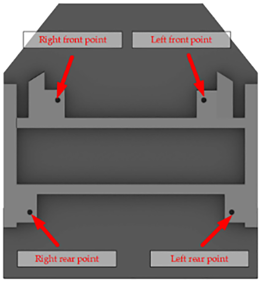
Diagram of suspended measurement points in the driver’s cab.

Figure 4.

Suspension acceleration test points.

Figure 5.

Cab noise test.

The suspended acceleration signal in the cab obtained through time-frequency transformation is shown in Figure 6. In the subsequent research, it is necessary to load this set of vibration data to the corresponding position of the finite element model to solve the vibration response of the cabin, laying the foundation for the subsequent acoustic response analysis.

Figure 6.

(a) Left front suspension acceleration, (b) left rear suspension acceleration, (c) right front suspension acceleration, and (d) right rear suspension acceleration.

The collected in-cabin noise signal, once transformed into the time-frequency domain, is depicted in Figure 7. In the following research, it is essential to compare and analyze this data with the simulated acoustic response of the cabin interior to validate the accuracy of the finite element model and boundary element model.

Figure 7.

Driver’s cabin interior noise curve.

Finite element model validation

Finite element modeling

The dimensions of the cab of a certain type of loader are as follows: 1610 mm in length, 1496 mm in width, and 1612 mm in height. When establishing the finite element model, some structures such as chamfers, flanges, and holes, which have little effect on the stiffness and mechanical performance of the cab, are simplified and removed due to the complex structure of the cab. The main structure of the cab is composed of steel panels, columns, beams, and glasses. The cab is meshed with an average mesh cell size of 10 mm. The doors and other components are connected rigidly. The established finite element model of the body-in-white is shown in Figure 8(a). The windshield glasses are also rigidly connected to the cab body, and the finite element model is shown in Figure 8(b). The windshield is also rigidly attached to the cab body. The finite element model is shown in Figure 8(b). Finite element model mesh inspection criteria as shown in Table 1. Among them, the number of quadrilateral elements is 253,902, and the number of triangular elements is 102, accounting for 0.04% of the total. The material of the cab body is Q235, with an elastic modulus of 210 GPa, a density of 7850 kg/m³, and a Poisson’s ratio of 0.3. The elastic modulus of the windshield glasses is 60 GPa, with a density of 2500 kg/m³, and a Poisson’s ratio of 0.23.

Figure 8.

(a) The finite element model of the body-in-white and (b) the finite element model of the entire cab.

Table 1.

Mesh quality check requirements.

Name	Standard	Name	Standard
Curved angle	≤15°	Interior angle	≤40°
Aspect ratio	≤5	Quadrilateral	45°–130°
Jacobi	>0.6	Triangle	30°–100°

Numerical analysis

Modal analysis

Modal analysis is a commonly used and effective method in modern engineering analysis. Through modal analysis, one can intuitively understand the characteristics of the cab structure, gain a preliminary insight into the dynamic properties of the structure and the rationality of the design, laying the foundation for subsequent solutions to vibration frequency response, and acoustic response.

The established structural finite element model will be imported into Abaqus software. Modal analysis steps will be configured, and the Lanczos method will be utilized to extract the free modes of the cabin within the frequency range of 0–500 Hz. Table 2 shows some of the calculated modal results of the cab structure, including the results of the first six orders of intrinsic modes except for the rigid body modes, and the modal results at the frequencies where the acceleration signals have obvious peaks (e.g. 39, 117, 175 Hz, etc.).

Table 2.

Cab modal shapes at different frequencies.

Modal order	1	2	3	4
Figure
Fre (Hz)	10.374	11.901	15.360	16.355
Property	Vibration occurs in internal rear panel	Vibration occurs in external rear fence	Vibration occurs in external rear fence	Vibration occurs in top panel
Modal order	5	6	7	18
Figure
Fre (Hz)	21.494	26.194	27.336	39.125
Property	Vibration occurs in external rear fence	Vibration occurs in internal rear panel	Vibration occurs in the internal roof panel and front windshield	Vibration occurs in windshield, door panel, and rear panel
Modal order	91	108	193	222
Figure
Fre (Hz)	105.54	117.12	174.84	195.21
Property	Vibration occurs in roof panel, rear bumper, and rear windshield	Vibration occurs in roof panel, rear bumper, and rear windshield	Vibration occurs in rear windshield and door panels	Vibration occurs in roof panel and front windshield

In the frequency range of 0–500 Hz, a total of 716 modes of the cabin were calculated, indicating a high modal density. The low-frequency modes of the cabin structure suggest that it is susceptible to external excitations causing structural vibrations. Concentration of natural frequencies within a narrow range can exacerbate resonance issues. As a result, the cabin is prone to significant vibrations from external excitations, which is not conducive to reducing structural noise within the cabin.

From the mode shapes depicted above, it can be concluded that the natural mode shapes exhibit local vibrations, primarily in areas covered by panels, including the internal rear panel, internal roof panel, external rear panel, external roof panel, and the left and right door panel areas. The pillars and beam structures of the cabin do not exhibit local vibrations.

Vibration response calculations and validation of finite element model accuracy

Vibration response calculations

Due to the high dimensionality of the structural model (approximately 250,000 nodes), modal methods were used for dynamic analysis. This method uses the structural modes to decouple the equation system, significantly reducing the computational time and memory requirements compared to direct methods. Therefore, step 1 is to solve the modal of the cab’s finite element model, and step 2 is to calculate the vibration response based on the modal method. In addition, the experimentally measured acceleration is applied as the load for the finite element model. In order to ensure a better calculation accuracy, it is generally necessary to retain all the modes within the frequency range of the highest external load, so this paper sets the modal frequencies involved in the calculation to be 0–500 Hz. The dynamic response of the structure is solved using the commercial finite element software Abaqus.

Figure 9 shows the addition of boundary conditions to the four suspension positions of the finite element model in the cab, and the experimentally measured vibration acceleration at these four suspension positions is applied. Figure 10 shows the results of the dynamic response in step 2, displaying the vibration velocity response cloud at the selected multi-peak frequencies.

Figure 9.

Schematic diagram of load addition.

Figure 10.

Vibration response contour was at: (a) 31 Hz, (b) 39 Hz, (c) 56 Hz, (d) 98 Hz, (e) 105 Hz, (f) 117 Hz, (g) 156 Hz, (h) 175 Hz, and (i) 195 Hz.

Validate the finite element model

A point on the floor plate was selected as one of the vibration acceleration acquisition points in the cab vibration test section. After obtaining the calculation results of the vibration response of the cab, a node is selected at the same position of the bottom plate on the finite element model, and the vibration acceleration response curve is exported and compared with the vibration data measured at this point in the test, which is used to verify the precision and accuracy of the finite element model. As shown in Figure 11, the test vibration acceleration curve and the simulation calculated vibration acceleration curve at this point have obvious peaks at several frequencies, such as 31, 39, 59, 97, 117, 136, 155, 175, 195 Hz, etc. The vibration acceleration amplitude simulation results at the reference point and the experimental test results basically correspond to each other in terms of the main peak frequency, which can better reflect the accuracy of the established finite element model of the cab. There is a certain difference in amplitude between the two, which is related to the experimental test error and the simplification of the model and the existence of damping parameters in the simulation process.

Figure 11.

Base plate acceleration test curve and calculation curve.

Acoustic response analysis and validation of boundary element model accuracy

The software LMS Virtual.Lab is widely used in the study of NVH performance of vehicles, integrating modules such as the acoustic finite element method and the acoustic boundary element method, as well as dynamic response analysis, making it a professional acoustic analysis software. Figure 12 illustrates the process of acoustic response calculation. In this study, the acoustic boundary element method is utilized to compute the structural radiation noise inside the vehicle cabin. Before the calculation, it is necessary to extract the acoustic cavity boundary model of the cabin, then convert the vibration response calculation results of the cabin structure into acoustic boundary conditions, set the response field points, and finally obtain the simulation results of the acoustic response inside the cabin.

Figure 12.

The process of acoustic response calculation.

As shown in Figure 13, the acoustic BEM of the cab cavity is extracted, in which the unit length is 50 mm and the number of quadrilateral units is 6111. The main material of the acoustic cavity is air, with a speed of 340 m/s and a density of 1.22 kg/m³. Defining the driver’s left ear location as a field point in the model. Use the previously calculated acceleration of the panels as the boundary condition for acoustic response and set the frequency range for solving as 20–200 Hz with a step size of 0.5 Hz. The comparison of simulated results and experimental results of the driver’s left ear sound pressure level is shown in Figure 14.

Figure 13.

Cab boundary element model.

Figure 14.

Driver’s left ear calculated sound pressure level curve and tested sound pressure level curve.

In Figure 14, the sampling frequency of the experimental data is much higher than the output frequency step size of the simulation results, resulting in a larger number of data samples in the experiment compared to the simulation calculations. This leads to differences in the final representation of the two curves. There are also differences between the two curves due to external noise interference during the experiment and the difficulty in determining certain parameters (such as modal damping parameters) when establishing the finite element model and boundary element model of the cabin.

However, despite these differences, the experimental curve and the calculated curve show the same trend in the frequency range of 20–200 Hz. Furthermore, at multiple frequencies such as 39 Hz (18th mode), 117 Hz (108th mode), 175 Hz (193rd mode), and 195 Hz (222nd mode), both curves exhibit noticeable noise peaks. Therefore, it can be concluded that the established Finite Element-Boundary Element (FEM-BEM) model is highly accurate.

Analysis and optimization

Panel acoustic contribution analysis

The generation of peak noise levels is usually due to two reasons: first, the suspended excitation of the driver’s cab itself has peaks, and second, the resonance between the natural frequency of the driver’s cab and the sound cavity. From Figure 15, the frequencies at which peak sound pressure levels occur are 31, 39, 59, 98, 105, 156, 175, and 195 Hz. Both the analog calculation and experimental test results in Figure 8 indicate that the sound pressure level in the loader’s cab reaches a maximum of 68.11 dB at 117, 31, 39, 59, 98, 105, 156, 175, and 195 Hz. By comparing the collected acceleration signals from the experimental tests, it can be observed that at these frequencies, the acceleration signals also exhibit relatively high peak values.

Figure 15.

Peak annotation chart of acoustic response calculation curve.

After the excitation is applied to the suspended position of the finite element model, the cloud map of vibration response speed for each peak frequency is shown in Figure 10. The vibration modes of the cab are all manifested as the vibration of the rear wall panel, roof panel, door panel, and the surrounding windshield, all of which are basically manifested as the vibration of the panels, with no vibration forms shown by the skeletal structures such as beams and columns. Therefore, the contribution of the panels to the sound pressure level calculation results for each peak frequency is analyzed. The panels that contribute significantly to the peak noise at a frequency of 39 Hz are the left and right door glass and the left and right door panels, with the glass area contributing approximately twice as much as the door panels. The peak noise at a frequency of 59 Hz mainly comes from the front panel, while the bottom panel and rear windshield contribute significantly to the peak noise at a frequency of 105 Hz. The peak noise at a frequency of 156 Hz is mainly due to the vibration of the front windshield, and the peak noise at a frequency of 175 Hz mainly comes from the rear windshield, contributing approximately half of the total contribution. The remaining frequency peak noise panel contributions are a combination of the top panel, bottom panel, rear panel, front panel, and glass panels, with the structural column panel contributions almost being zero. Comparing the contribution analysis of the panel with the dynamic response results in Figure 10, it can be seen that the regions with larger structural vibration response amplitudes at peak frequencies correspond to the areas with larger panel contributions. This also confirms that the noise generated by vibration is the main source of cab noise in the frequency range of 20–200 Hz.

The envelope of the acoustic cavity in the driver’s cab was disassembled into 14 main panels for acoustic contribution analysis. The panels are labeled as follows: top panel 1, bottom panel 2, rear panel 3, front panel 4, front windshield panel 5, left front structural pillar panel 6, left rear structural pillar panel 7, left door windshield panel 8, left door panel 9, right front structural pillar panel 10, right front structural pillar panel 11, right door windshield panel 12, right door panel 13, and rear windshield panel 14. Figure 16 shows the disassembled main panels of the driver’s cab acoustic cavity shell.

Figure 16.

Disassembled envelope of the acoustic cavity system of a cab.

From the Figure 17, the noise at 117 Hz is caused by the vibration of multiple panels, including the top panel, bottom panel, rear panel, front bulkhead, left and right door panels, and surrounding glass panels. However, due to the special nature of glass materials, their thickness is usually fixed, and the front bulkhead is directly bonded to the glass structure, so its thickness is related to the glass thickness. Therefore, the front bulkhead and glass panels are not within the scope of optimizing the panels. As a result, panel 1, panel 2, panel 3, and panel 9 are designated as key panels in this study. Furthermore, since the driver’s cab is usually symmetrical in structure, panel 9 and panel 13 are considered to be the same design variable and are taken into account during the subsequent optimization process.

Figure 17.

The contribution of the panels at: (a) 39 Hz, (b) 117 Hz, (c) 156 Hz, and 175 Hz.

Establishment of the optimization model

According to the analysis results of the cab panels acoustic contribution, the thickness of the panel was determined as the design variable. The thickness of panel 1, panel 2, and panel 3 are defined as design variables x₁, x₂, x₃ respectively. Panel 9 and panel 13 are symmetric, and their thickness are considered as a design variable defined as x₄, making a total of four design variables. The maximum sound pressure level response occurs at 117 Hz, so reducing this maximum noise is set as the optimization objective. To avoid resonance with road excitations, the first natural frequency should not decrease during optimization (the first natural frequency of the original model is 10.374 Hz). At the same time, this step should ensure that the weight increment of the cab is less than 3%. Based on the previous analysis, the optimization model is established as follows.

\begin{matrix} Min : f_{1} (x_{1}, x_{2}, x_{3} x_{4}) \leq 68.11 dB \\ f_{2} (x_{1}, x_{2}, x_{3} x_{4}) \geq 10.374 Hz \\ f_{3} (x_{1}, x_{2}, x_{3} x_{4}) \leq 1.03 m_{0} \\ 2.5 \leq x_{1} \leq 3.5 (mm) 7.5 \leq x_{2} \leq 8.5 (mm) \\ 2.5 \leq x_{3} \leq 3.5 (mm) 4.5 \leq x_{4} \leq 5.5 (mm) \end{matrix}

In the above optimization model f₁ represents the sound pressure level at 117 Hz; f₂ represents the first natural frequency; f₃ represents the weight of the driver’s cab; m₀ represents the mass of the original model. x₁, x₂, x₃, and x₄ are the thicknesses of the key panels, serving as design variables.

Establishment of the approximate model on the basis of the Response Surface Model

After the experimental design and sample extraction, it is necessary to establish an approximation model. An approximation model is a mathematical model constructed with a small computational cost and short computational time, while maintaining a similar calculation result to the numerical analysis result without reducing the computational accuracy. Common methods for constructing approximation models include Kriging Model, Response Surface Model (RSM), Radial Basis Function (RBF), etc.

Response surface methodology is a technique that uses a rational experimental design to extract sample data points, establishing a nonlinear relationship between design variables and response functions.¹⁸ The approximate model constructed using response surface methodology can utilize fewer sampling iterations, obtaining a relatively precise approximation of the relationship between design variables and response functions, expressed through a polynomial regression equation.

According to equation (10), this paper establishes a second-order response surface model between design variables and response functions.

f_{k} = β_{0} + \sum_{i = 1}^{n} β_{i} x_{i} + \sum_{i = 1}^{n} β_{ii} {x_{i}}^{2} + \sum_{i < j}^{n} β_{ij} x_{i} x_{j}

(10)

In the equation (10), f_k is the response target function; x_i and x_j are the ith and jth design variables, i and j = 1, 2, 3, 4. β₀ is the constant term; β_i, β_ii, and β_ij are the coefficients of the respective terms; n is the number of design variables.

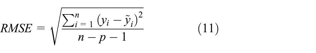
The study used the Latin square design method as the sampling method and established a high-fidelity approximation model. Table 3 shows the selected sample data for the Latin square and the numerical values of the simulation calculations for f₁, f₂, and f₃ for each sample. Afterward, it is necessary to evaluate the fitting accuracy of the established approximate model. Cross-validation is a method used in the fields of statistics and machine learning to estimate the generalization ability of models. By using cross-validation, overfitting and underfitting problems can be addressed, allowing for an effective and reasonable assessment of the predictive accuracy of the approximate model.¹⁹ The precision of the approximate model is usually evaluated using RMES and R². Their expressions are as follows¹²:

RMSE = \sqrt{\frac{\sum_{i = 1}^{n} {(y_{i} - {\tilde{y}}_{i})}^{2}}{n - p - 1}}

(11)

R^{2} = 1 - \frac{\sum_{i = 1}^{n} {(y_{i} - {\tilde{y}}_{i})}^{2}}{\sum_{i = 1}^{n} {(y_{i} - {\bar{y}}_{i})}^{2}}

(12)

Table 3.

Sample points and calculation results.

No.	x ₁ (mm)	x ₂ (mm)	x ₃ (mm)	x ₄ (mm)	f ₁ (dB(A))	f ₂ (Hz)	f ₃ (kg)
1	2.868	7.500	3.342	4.868	67.76	9.9338	575.06
2	2.816	7.553	2.763	4.553	65.29	9.7589	565.57
3	2.500	7.605	2.553	5.237	65.30	8.6913	562.85
4	2.763	7.658	2.711	5.026	65.55	9.5808	567.88
5	2.605	7.711	2.500	5.500	65.28	9.0474	566.06
6	2.553	7.763	3.447	5.447	66.50	8.717	578.86
7	3.079	7.816	3.079	4.816	66.41	10.636	577.79
8	2.711	7.868	3.184	4.605	65.20	9.406	574.35
9	2.974	7.921	2.868	5.184	65.85	10.288	576.76
10	2.658	7.974	2.816	4.974	64.03	9.2269	571.81
11	3.395	8.026	2.605	5.132	66.01	11.645	579.37
12	3.342	8.079	2.974	4.500	65.17	11.489	581.35
13	2.921	8.132	3.500	5.079	65.96	10.111	586.98
14	3.026	8.184	3.237	4.658	64.69	10.461	583.23
15	3.447	8.237	3.395	4.921	66.81	11.775	592.53
16	3.237	8.289	3.026	5.289	65.41	11.155	587.36
17	3.500	8.342	3.289	4.711	65.96	11.844	592.02
18	3.132	8.395	2.921	5.395	64.57	10.811	586.51
19	3.184	8.447	2.658	4.763	62.11	10.981	581.06
20	3.289	8.500	3.132	5.342	65.04	11.323	592.41

$y_{i}$ , ${\tilde{y}}_{i}$ , and ${\bar{y}}_{i}$ are the measured value, predicted value, and average of the measured value; n represents the number of measurement points, and p represents the number of degrees of freedom, which is equal to the number of variables minus 1. RMSE represents the variance between the measured values and the predicted values. When RMSE is small, the accuracy of the approximate model is high. The closer R² is to 1, the higher the accuracy of the approximate model.

Table 4 presents the errors of the response surface model, which assesses the accuracy of the model. The variables f₁, f₂, and f₃ correspond to the sound pressure level at 117 Hz near the driver’s ear, the first-order modal frequency of the driver’s cab, and the total mass of the driver’s cab, respectively. The results suggest that the response surface model is adequately accurate and can be utilized for further multi-objective optimization.

Table 4.

Response surface model accuracy evaluation.

Response	RMSE	R ²
f ₁	0.0335	0.9715
f ₂	0.0421	0.9824
f ₃	0.0000	1.0000

Optimization result and analysis

NSGA-II algorithm is widely used in selective combinatorial optimization problems, with the advantages of fast convergence speed, low computational complexity, and high robustness.^20,21 It is an improvement based on the genetic algorithm (NSGA) proposed by Deb et al.²² In the optimization model established above, there are four design variables and three response functions, with specified ranges and constraints for both design variables and response functions. As shown in Figure 18, the response surface methodology will be used to construct a nonlinear mathematical model of the inputs and outputs, and the NSGA-II algorithm will be used to solve the established mathematical model to solve the multi-objective optimization problem.

Figure 18.

Flowchart of the optimization process.

The NSGA-II algorithm is used to solve the approximate model established in the above sections in this article. The corresponding algorithm settings for the solution are shown in Table 5. According to the solution of the NSGA-II algorithm, the design variables of the optimized approximation model are x₁ = 2.541 mm, x₂ = 7.616 mm, x₃ = 3.013 mm, x₄ = 4.751 mm. The main support structure of the loader cab consists of bottom beams, reinforcement ribs, and other structures. Minor variations in plate thickness will not affect safety. However, considering the issue of panels thickness specifications in practical engineering problems, the optimized results are rounded to x₁ = 2.5 mm, x₂ = 7.6 mm, x₃ = 3.0 mm, x₄ = 4.8 mm.

Table 5.

Optimization parameter settings for NSGA-II.

Option	Value
Population size	12
Number of generations	20
Crossover probability	0.9
Crossover distribution index	10
Nutation distribution index	20

The final optimized results were imported into the approximate model and the finite element model for calculation, and compared with the response values of the original model. The results are shown in Table 6, with errors all smaller than 1%, proving the effectiveness of the approximate model.

Table 6.

Comparison of optimization results.

Compare items	x ₁ (mm)	x ₂ (mm)	x ₃ (mm)	x ₄ (mm)	f ₁ (dB(A))	f ₂ (Hz)	f ₃ (kg)
Optimal value
Original value	3.0	8.0	3.0	5.0	67.11	10.374	578.99
Approximate model	2.5	7.6	3.0	4.8	65.78	10.388	566.719
FEM	2.5	7.6	3.0	4.8	65.21	10.374	566.72
Approximate model error (%)					0.8665	0.0134	0.0013

The human body being an organic life form, the impacts of vibrations on it are indeed quite intricate. In a setting with low-frequency vibrations, the body can display physiological responses and even present health risks. However, as the frequency of vibrations rises, the physiological effects on the human body tend to decrease gradually, eventually only affecting specific body parts in contact with the vibrations. It’s interesting to note that the resonant frequencies of various human organs all fall within the 200 Hz range. In spaces with higher sound pressure levels, enclosed areas are more likely to resonate with structures, amplifying the influence of vibrations on the human body and worsening discomfort.

Apart from causing physiological discomfort, several studies have pointed out that low-frequency noise can have a more pronounced impact on human emotions compared to high-frequency noise, leading to increased annoyance and influencing cognitive abilities, particularly in the 50–300 Hz frequency range. Following the optimization of the structure, the acoustic response curve, when compared to the original cabin structure, as shown in Figure 19, displays a decreasing trend in the 20–200 Hz frequency range. For instance, the peak sound pressure level at 117 Hz frequency decreased from 68.11 to 65.21 dB, marking a reduction of 4.26%. At 29 Hz, the sound pressure level decreased from 36.79 to 28.6 dB, and at 58 Hz, the noise peak dropped from 31.26 to 28 dB. However, at specific frequencies such as 105 Hz, the noise levels remained unchanged. This is because the peaks of these noises are caused by the vibration of glass plates, and their thickness was not altered during the optimization process. Notably, the optimization effects are more prominent in the low-frequency range, suggesting that the acoustic environment of the optimized cabin surpasses that of the original cabin.

Figure 19.

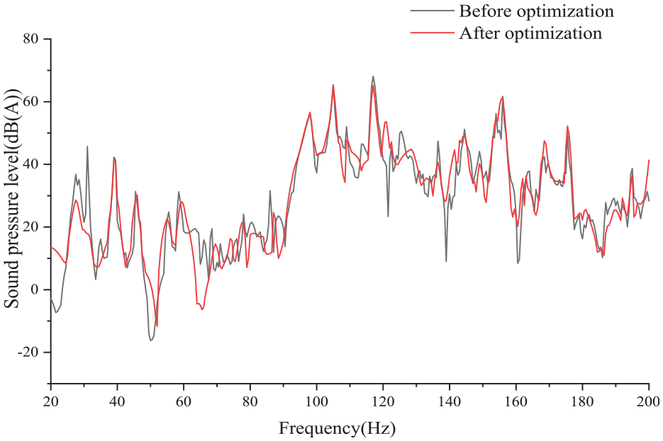
Comparison of optimization results.

Conclusions

This article introduces an optimization method for the low-frequency noise structure of a loader cab based on a response surface method approximation model. The loader cab is modeled using the finite element method and acoustic boundary element method. Vibration acceleration signals obtained from experimental measurements on the loader cab and sound pressure level signals near the driver’s ear are used as excitations to solve the structural dynamic response of the cab using the finite element model. The structural dynamic response results are then used as the acoustic boundary conditions of the acoustic boundary element model, with the driver’s ear position set as the acoustic response field point to calculate the acoustic response curve inside the cab. The accuracy of the established finite element model is verified by comparing the calculation results with the experimental test results, which can be used for subsequent optimization analysis. According to the results of the PACA analysis, the panels that contribute the most to the driver’s left ear in the low-frequency range are the roof, floor, rear panel, and door panel. The thickness of these four panels is taken as the design variables x₁, x₂, x₃, x₄, and an optimization model is established. The response surface method is used to establish an approximation model, and the NSGA-II algorithm is used to solve the optimization model and obtain the optimized thickness of the key panels.

Based on the comparison and analysis of the optimized left ear sound pressure level curve of the driver, the peak at 117 Hz decreased by 2.9 dB after optimization, showing a decreasing trend in the frequency range of 20–200 Hz. However, at specific frequencies such as 105 Hz, the noise levels remained unchanged. This is because the peaks of these noises are caused by the vibration of glass plates, and their thickness was not altered during the optimization process. The results indicate that the optimization method based on the approximate model established in this study is effective.

Footnotes

Handling Editor: Aarthy Esakkiappan

Declaration of conflicting interests

The author(s) declared no potential conflicts of interest with respect to the research, authorship, and/or publication of this article.

Funding

The author(s) disclosed receipt of the following financial support for the research, authorship, and/or publication of this article: Shanxi Provincial Science and Technology Major Project; Item No. 20181102002, and Taiyuan University of Science and Technology Graduate Education Innovation Project; Item No. SY2023037.

ORCID iDs

Qinhong Fan

Hongquan Dong

References

Stodola

. Noise reduction in the cab of a special vehicle. Def Sci J 2022; 72: 450–458.

Noh

H-M

. Prediction and reduction in vehicle noise by frequency response function–based substructuring. Adv Mech Eng 2016; 8: 1687814016642668.

Liao

Zuo

Meng

, et al. Research on the technology of noise reduction in hybrid electric vehicle with composite materials. Adv Mech Eng 2018; 10: 1687814018766916.

Zhou

Wang

. Vibration and noise damping treatment for an excavator cab. Adv Mater Res 2014; 889–890: 455–458.

Han

Guo

, et al. Interior sound field refinement of a passenger car using modified panel acoustic contribution analysis. Int J Automot Technol 2009; 10: 79–85.

Feng

Zheng

Wang

, et al. Low-frequency acoustic-structure analysis using coupled FEM-BEM method. Math Probl Eng 2013; 2013: 583079.

Sun

Liu

, et al. Panel acoustic contribution analysis in automotive acoustics using discontinuous isogeometric boundary element method. Comput Model Eng Sci 2023; 135: 2307–2330.

Jiao

Nguyen

Zhang

. Acoustic-structure modeling and analysis of an engineering machinery cab based on the hybrid method and experimental investigations. J Braz Soc Mech Sci Eng 2020; 42: 1–8.

Zhang

, et al. Low-frequency noise inside metro: contribution analysis and noise control treatment. J Mech Sci Technol 2023; 37: 2821–2830.

10.

Guo

Zhang

Zhao

, et al. Interior structure-borne noise reduction by controlling the automotive body panel vibration. Proc IMechE, Part D: J Automobile Engineering 2012; 226: 943–956.

11.

Liu

Zhou

Zhu

, et al. Optimization of noise transfer path based on the composite panel acoustic and modal contribution analysis. Complexity 2021; 2021: 3059865.

12.

Zhang

Huang

, et al. Low-noise structure optimization of a heavy commercial vehicle cab based on approximation model. J Low Freq Noise Vib Active Control 2018; 37: 987–1002.

13.

Dong

Sun

. Application of Kriging model to gear wear calculation under mixed elastohydrodynamic lubrication. Machines 2022; 10: 490.

14.

Wang

, et al. A novel surrogate-based aerodynamic optimization method using field approximate model. Proc IMechE, Part G: J Aerospace Engineering 2019; 233: 883–895.

15.

Zhou

, et al. Air duct optimization design based on local turbulence loss analysis and IMOCS algorithm. Machines 2023; 11: 129.

16.

. Study on vibro-acoustic characteristics and optimization design of loader cab. MS Dissertation, Tianjin University, China, 2014. (in Chinese)

17.

Citarella

Federico

Cicatiello

. Modal acoustic transfer vector approach in a FEM–BEM vibro-acoustic analysis. Eng Anal Bound Elem 2007; 31: 248–258.

18.

Dong

XCA

, et al. Prediction model of punching springback of windshield beam based on response surface method. Rare Met Mater Eng 2021; 50: 1611–1616.

19.

Wen

Yang

, et al. An approximation modeling method of lunch vehicles improved by fast cross-validation. Astronaut Sin 2022; 43: 225–237. (in Chinese)

20.

Chen

Liu

, et al. Improved NSGA-II and its application in BIW structure optimization. Adv Mech Eng 2023; 15: 16878132221150588.

21.

Zhang

Sun

, et al. A comprehensive survey on NSGA-II for multi-objective optimization and applications. Artif Intell Rev 2023; 56: 15217–15270.

22.

Deb

Pratap

Agarwal

, et al. A fast and elitist multi objective genetic algorithm: NSGA-II. IEEE Trans Evol Comput 2002; 6: 182–197.

Research on prediction and optimization of low-frequency noise in loader cabs

Abstract

Keywords

Introduction

Basic theory

Frequency response theory

Panels Acoustic Contribution Analysis theory

Experimental data collection

Finite element model validation

Finite element modeling

Numerical analysis

Modal analysis

Vibration response calculations and validation of finite element model accuracy

Vibration response calculations

Validate the finite element model

Acoustic response analysis and validation of boundary element model accuracy

Analysis and optimization

Panel acoustic contribution analysis

Establishment of the optimization model

Establishment of the approximate model on the basis of the Response Surface Model

Optimization result and analysis

Conclusions

Footnotes

Declaration of conflicting interests

Funding

ORCID iDs

References