Few-shot bearing fault diagnosis method based on an EEMD parallel neural network and a relation network

Abstract

Bearing fault diagnosis presents challenges, such as insufficient fault samples and significant fault data distribution variation in different bearing operating conditions. These problems cause traditional deep learning models to show poor generality and accuracy during bearing fault diagnosis. To address these challenges, this paper proposed a few-shot bearing fault diagnosis method based on an Ensemble Empirical Mode Decomposition (EEMD) parallel neural network and a relation network (RN). First, the original bearing fault vibration signal was decomposed by EEMD, while the decomposed signal components were processed via Short Time Fourier Transfor (STFT) to obtain a two-dimensional time-frequency feature map. Then, a parallel neural network was used for initial fault feature extraction, after which the extracted features were fused to construct a more accurate multi-dimensional fault feature map. A more precise fault feature vector was generated via the feature embedding module of the RN, and the fault features of the support and query sets were stitched to create a fault feature vector set. Finally, the relation module of the RN was used for the nonlinear distance determination of the fault feature vector set and to generate the relation score for the few-shot variable condition bearing fault diagnosis. In this paper, EEMD module is introduced into RN to construct multi-dimensional fault characteristics of the original fault signal. Original signal decomposition, STFT transformation and splicing effectively improve the randomness and blindness of convolution operations, improve the accuracy of fault feature extraction in RN, and thus improve the overall diagnostic performance of the model. The experimental results showed that the proposed model obtained higher diagnostic accuracy than the matching network (MN) and RN meta-learning fault diagnosis (MLFD) methods. The accuracy of fault diagnosis of the model in 5Way-Nshot is >80%, and the accuracy of fault diagnosis in 5Way-10shot is the highest at 95.2%.

Introduction

Bearings are important components in rotating machinery and equipment that support the rotating body. Therefore, timeous fault diagnosis is essential since bearing health determines the efficient and stable operation of equipment. Song et al. ¹ proposed a fault diagnosis method by combination of finite element method (FEM), wavelet packet transform (WPT) and support vector machine (SVM). The bearing signal is obtained by finite element model, the vibration signal is decomposed by wavelet transform, and the training sample is finally used in support vector machine for classification. Liu et al. ² proposed a personalized fault diagnosis method using finite element method (FEM) simulation and ELM . Experimental results show that the fault diagnosis accuracy of this method can reach >85%. Vashishtha et al. ³ proposed A novel approach for identifying the impeller defects in the centrifugal pump has been demonstrated by extracting the single-valued neutrosophic cross-entropy (SVNCE) of adaptive chirp mode decomposition (ACMD). Compared with EMD, EEMD and other methods, the superiority of this method is proved by experiments.

The rapid development of computer technology has increased the research application of deep learning for fault diagnosis. Deep learning models are sensitive to data features and can extract deeper features from the original data. Rehman et al. ⁴ proposed RAAGR2-Net to effectively segment brain tumor regions. The model enriches the feature representation by combining the information of multiple feature graphs. The effectiveness of the method is verified by experiments. Yu et al. ⁵ proposed a novel loss-balanced parallel decoding network(PadNet) used for macular edema segmentation. Kumar et al. ⁶ proposed a deep learning method for the identification of engine defects of two-wheeler vehicle. This method uses wavelet synchronous compression transform (WSST) to process the training and test data. Then the cost function of convolutional neural network (CNN) is modified, experiments show that the accuracy of this method is higher than other models. Vashishtha and Kumar ⁷ proposed a novel unsupervised learning method called general normalized sparse filtering (GNSF) based on Wasserstein distance with maximum mean discrepancy (MMD) for fault diagnosis. This method can successfully identify various health conditions of centrifugal pumps and Pelton wheels. Vashishtha and Kumar ⁸ proposed a filter based feature selection technique is introduced into the machine learning model, and the fault classification of centrifugal pump vibration signal data set is successfully carried out. Fault diagnosis methods based on deep learning have been widely used, but these methods all require a large number of fault samples for training models. However, the operating conditions of mechanical equipment are often in excellent operational condition, leading to a small number of fault samples and unbalanced data. In addition, due to the harshness and complexity of the working environment, equipment often operates in unstable conditions, leading to significant time variability. Therefore, bearing fault diagnosis represents a typical problem in few-shots and variable operating conditions, and training a diagnostic model to improve accuracy requires further exploration.

Meta-learning ⁹ is a cutting-edge deep-learning technique that ascertains meta-knowledge from many priori tasks, allowing the model to learn new tasks more rapidly. Therefore, the meta-learning technique can be used for variable service gear fault diagnosis. Current meta-learning research focuses on optimization, metrics, and models. ¹⁰ Li et al. ¹¹ proposed an agnostic-based meta-learning fault diagnosis (MLFD) model, which is trained to obtain prior knowledge by initializing parameters based on multiple fault classification tasks in known operating conditions. This information is used to rapidly and accurately diagnose few-shot bearing faults in unknown conditions. However, determining optimal initial hyperparameters is challenging. Improper model parameter settings affect its convergence speed, ¹² while adjusting these criteria for a specific task is usually time-consuming and computationally expensive. Zhang et al. ¹³ proposed a few-shot bearing fault diagnosis method based on meta-learning twin networks using the metrics between samples from the same or different categories. Due to the complex and diverse frequency components of fault vibration signals and large changes in operating conditions, current fault diagnosis models based on meta-learning pay less attention to deep fault features and ignore the correlation between signals.

This paper proposes a few-shot bearing fault diagnosis method based on EEMD parallel neural and relation networks (RN) to address these challenges. The bearing fault samples are divided into data sets according to the meta-learning training mechanism, after which the raw bearing fault input data are decomposed via EEMD and processed using STFT. The decomposed fault signal components are transformed into a two-dimensional time-frequency feature map, which is passed through a parallel neural network containing a one-layered convolutional neural network. The fault features are fused with those initially processed to construct a more accurate multi-dimensional fault feature map, from which features are extracted using the embedding module in the RN. Next, the fault features of the support and query sets are spliced into a feature vector group. Finally, the corresponding similarity score is calculated via the relation module in the RN to determine the bearing fault diagnosis accuracy in few-shot variable conditions.

Theoretical basis

Meta-learning

Meta-learning is a deep learning-based approach that can effectively handle few-shot classification tasks. Unlike traditional supervised learning, which proportionally divides the dataset into training and test sets, meta-learning training and test sets display different data distributions, that is, no crossover between the data in these sets. Meta-learning uses a stage-based mechanism ¹⁴ for model training. Assuming the existence of a training set D, and define to select several samples from each category of the training set, the collection of these samples is called the Support set, and the other samples from the remaining samples of each category are selected, which is called the Query set. The data in the support set is labeled, the data in the query set is not labeled, and the support set and the query set share the same sample space. We use support sets to train the model and query sets to test the model. If N classes are randomly selected in the training set, K labeled samples for each class are selected as the support set S= $\{(x_i,y_i){\}}_{i=1}^M$ (M=N*K), And the remaining part of this class N sample is used as query set Q= $\{(x_j,y_j){\}}_{j=1}^C$ , it is called N-way K-shot situational training strategy.

The situational training strategy of meta-learning is divided into two stages: meta-training and meta-testing, as shown in Figure 1. In the meta-training stage, given multiple sub-training tasks, the categories of each task are not exactly the same, and the data of each sub-training task is divided into support set and query set, where the support set is divided into N categories, each category includes K pictures, and the model parameters of each sub-task are trained through the support set of multiple sub-tasks. The model performance is then tested and the parameters updated through the query set for each subtask. After a large number of task training, the model performs several new tasks similar to the meta-training stage in the meta-test stage. At this time, the categories in the new tasks have not appeared in the meta-training stage. The model uses the training data to classify the unlabeled test data.

Figure 1.

N-way K-shot situational training strategy.

Relation network

The RN ¹⁵ is a metric-based meta-learning method. Its structure is shown in Figure 2, which consists of two modules: the embedding module and the relation module. The embedding module mines the useful feature information in the image. When the network input is an image, the embedding module extracts the respective support and query set features, which are represented as:

$${\mathrm{f}}_{\phi }({\mathrm{x}}_{\mathrm{i}})={\mathrm{G}}_{\mathrm{e}}({\mathrm{x}}_{\mathrm{i}};{\theta }_{\mathrm{e}})$$

(1)

$${\mathrm{f}}_{\phi }({\mathrm{x}}_{\mathrm{j}})={\mathrm{G}}_{\mathrm{e}}({\mathrm{x}}_{\mathrm{j}};{\theta }_{\mathrm{e}})$$

(2)

Figure 2.

The RN structure diagram.

Here, $f_{\phi }$ ( $x_i$ ) is the ith sample feature of the support set, $f_{\phi }(x_j)$ denotes the jth sample feature of the query set, $G_e(·;·)$ signifies the embedding module, and ${\theta }_e$ represents the corresponding parameters. Subsequently, the feature vectors of the query set $f_{\phi }(x_j)$ and support set $f_{\phi }$ ( $x_i$ ) are stitched together and denoted as:

$${\mathrm{f}}_{\mathrm{con}}^{\mathrm{ij}}=\mathrm{C}({\mathrm{f}}_{\phi }({\mathrm{x}}_{\mathrm{i}}),{\mathrm{f}}_{\phi }({\mathrm{x}}_{\mathrm{j}}))$$

(3)

$C(·)$ denotes the splicing operation. The relation module processes the spliced feature vector set and generates the relation score corresponding to each class via the relation function $r_{\mathrm{ij}}$ , which is expressed as:

$${\mathrm{r}}_{\mathrm{i},\mathrm{j}}={\mathrm{g}}_{\varnothing }({\mathrm{f}}_{\mathrm{con}}^{\mathrm{ij}},{\theta }_{\mathrm{r}})$$

(4)

$g_{\varphi }(·)$ denotes the relation module, which is used to calculate the similarity scores of the support and query set samples, while ${\theta }_r$ represents the corresponding parameter.

The specific structural parameters of the embedding and the relation modules in the RN are shown in Figure 3. The embedding module consists of four convolutional blocks and two pooling layers, while the relation module comprises two convolutional blocks, two pooling layers, and two fully connected layers with eight and one neuron, respectively. Each convolutional block consists of a convolutional, a batch normalization, and a ReLu layer.

Figure 3.

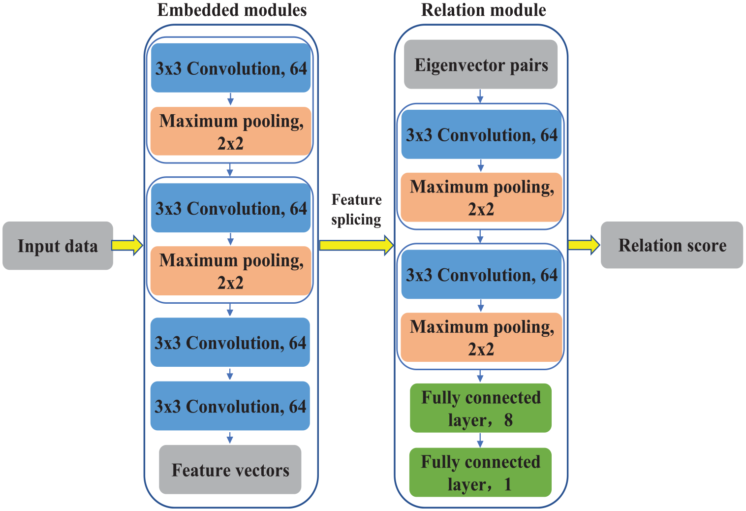
A diagram of the specific RN structural parameters.

Unlike traditional metrics, such as Euclidean and cosine metrics, RNs train a classifier with a learnable nonlinear distance metric to compute the degree of match between samples.

The RN uses the mean square error (MSE) as the loss function, expressed as follows:

$$\phi ,\varnothing <-\mathrm{argmi}{\mathrm{n}}_{\phi ,\varnothing }\sum _{\mathrm{i}=1}^{\mathrm{m}}\sum _{\mathrm{j}=1}^{\mathrm{n}}({\mathrm{r}}_{\mathrm{i},\mathrm{j}}-1({\mathrm{y}}_{\mathrm{i}}=={\mathrm{y}}_{\mathrm{j}}){)}^2$$

(5)

In equation (5), yi represents the true value of the support set sample and yj represents the predicted value of the query set sample. When the input query and support set samples belong to the same category, the function value output result is 1, while it is 0 when they form part of different categories.

EEMD-based signal decomposition

Wu and Huang ¹⁶ proposed an improved algorithm, namely Ensemble Empirical Mode Decomposition (EEMD), which solved the EMD to address the modal mixing challenge. The algorithm utilized the uniform frequency distribution properties of Gaussian white noise to offset the original signal noise, effectively suppressing the occurrence of the mixing phenomenon and obtaining a more accurate envelope. Furthermore, the variational modal function components were averaged to reduce the influence of white noise on the results. Therefore, the EEMD algorithm improved signal processing accuracy.

The signal steps are as follows:

• (1) Gaussian white noise z(t) is added to the original bearing fault signal x(t) to obtain a new bearing fault signal X(t):

$${\mathrm{X}}_{(\mathrm{t})}={\mathrm{x}}_{(\mathrm{t})}+{\mathrm{z}}_{(\mathrm{t})}$$

(6)

• (2) The EMD of X(t) is used to obtain the m eigenmodular function components Cj(t) and the residual components r(t):

$${\mathrm{X}}_{(\mathrm{t})}=\sum _{\mathrm{j}=1}^{\mathrm{m}}{\mathrm{C}}_{\mathrm{j}(\mathrm{t})}+{\mathrm{r}}_{(\mathrm{t})},(\mathrm{j}=1,2,...,\mathrm{m})$$

(7)

• (3) Add ith different Gaussian white noise z(t) to the original bearing fault signal to obtain ith new fault signals:

$${\mathrm{X}}_{\mathrm{i}(\mathrm{t})}=\sum _{\mathrm{j}=1}^{\mathrm{m}}{\mathrm{C}}_{\mathrm{ij}(\mathrm{t})}+{\mathrm{r}}_{\mathrm{i}(\mathrm{t})},(\mathrm{i}=1,2,...,\mathrm{n})$$

(8)

where t represents variable of time, i indicates the white Gaussian noise added for the ith time, Cij(t) represents the jth IMF component of the EMD after the i-th addition of Gaussian white noise.

• (4) The IMF components are averaged to attenuate the effect of added Gaussian white noise. The final IMF component obtained via EEMD decomposition is:

$${\mathrm{C}}_{\mathrm{j}(\mathrm{t})}=\frac{1}{\mathrm{n}+1}\sum _{\mathrm{j}=1}^{\mathrm{m}}{\mathrm{C}}_{\mathrm{ij}(\mathrm{t})}$$

(9)

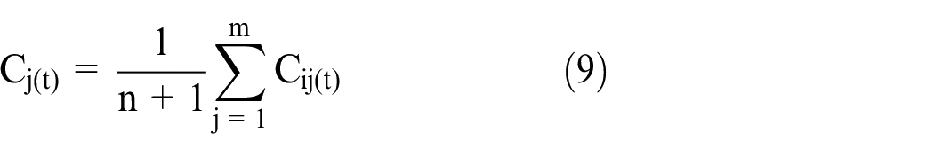
where Cj(t)-jth represents the IMF component of the original signal via EEMD.

The EEMD algorithm is simple and efficient and effectively reduces the interference of other complex signals. By decomposing the original vibration signal of the bearing, the algorithm obtains IMF and residual components for effective signal characterization. Compared with the EMD algorithm, the EEMD algorithm is more suitable for satisfying the input requirements of deep learning models, while the resultant multi-dimensional features aid the subsequent feature fusion. Using the EEMD algorithm for signal processing improves diagnostic accuracy and reliability, increasing fault diagnosis and prediction ability.

Figure 4 shows the corresponding fault times and frequency characteristics of each component after EEMD of the bearing fault signal following STFT variation.

Figure 4.

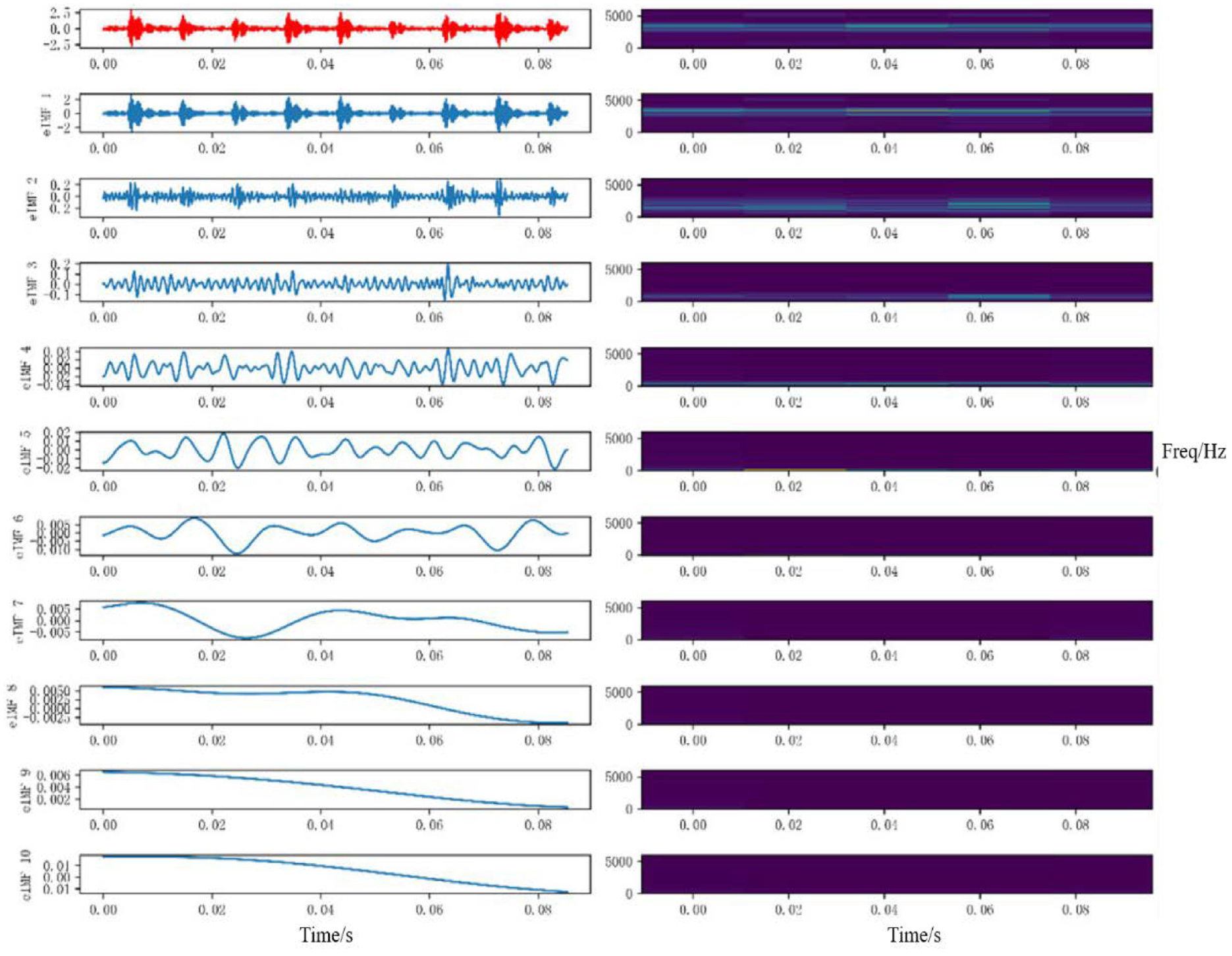
A schematic diagram of the signal after EEMD and STFT processing.

The construction of the improved RN fault diagnosis model

Fault diagnosis model

Bearing fault diagnosis using convolutional neural networks occurs as follows: First, the bearing fault signal is segmented into sliding windows, and the long sequence is cut into several shorter signal fragments. Second, the signal fragments are sequentially converted into a two-dimensional time-frequency map, satisfying CNN. Finally, the fault features are extracted and classified via convolutional layers on the feature map. This basic process is widely used in CNN-based fault diagnosis methods. However, when the bearing fault samples are small, CNNs are usually prone to overfitting, reducing the model robustness and generalization ability. Studies have shown that parallel convolutional neural networks may help address this problem in some fields. ¹⁷ Therefore, this paper proposes a few-shot bearing fault diagnosis model based on parallel neural networks and RNs according to the bearing fault vibration signal characteristics. The fault diagnosis model is shown in Figure 5.

Figure 5.

The parallel RN fault diagnosis model.

The model consists of several parallel convolutional neural networks that slice the original signal using a window with an overlap rate of 0.5 and a sliding window size of 1024. This generates the sample time series and increases the correlation between the faulty samples. As shown in Figure 5, the output feature maps of each channel are subjected to feature fusion. Since channel fusion occurs sequentially according to the EEMD order, it generates a relationship between the channel information and fault category correspondence to further highlight the fault features. The embedding module in the RN is used to extract the features from the newly fused fault features, while the relation module is used to calculate the similarity scores of the support and query sets and make predictions for fault classification and identification.

Troubleshooting process

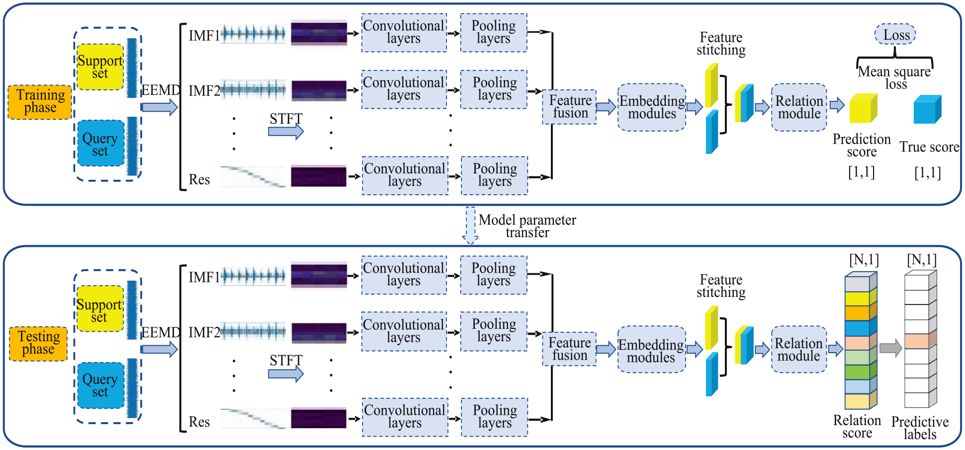
The few-shot fault diagnosis process (EMRN) based on a parallel neural network and an RN proposed in this paper is shown in Figure 6. The pre-processed fault data are divided into respective training and test sets, while the three data sets are divided into support and query sets. The training set is used for model pre-training. The input samples are pre-processed via EEMD and STFT and passed through a parallel neural network containing a one-layered convolutional neural network for processed fault feature fusion to obtain a more accurate and detailed fault feature map. The fused fault features are extracted using the RN embedding module, while the sample feature vectors of the support and query sets are stitched to form a feature vector set. The relation module calculates the feature vector similarity and outputs a similarity score in a range of [0,1], representing the degree of similarity between the samples. The subsequent model parameters are finally passed to the testing model to determine whether better fault diagnosis is achieved using the few-shot method. The training and testing processes are performed using the Adam optimizer, while the MSE loss function is used to evaluate the differences between the predicted and true scores.

Figure 6.

The few-shot fault diagnosis process based on a parallel neural network and RN.

Few-shot bearing fault diagnosis experiment

Data acquisition

This paper used the CWRU18 experimental bearing failure platform for the bearing failure simulation experiments to verify the efficacy of the EMRN. As shown in Figure 7, the experimental platform mainly consisted of a motor, torque sensor, and dynamometer. EDM technology was used to simulate bearing failure in actual working conditions. Single-point failures of different sizes were established in the inner ring, outer ring, and ball body of the bearing, with respective failure size diameters of 0.007, 0.014, 0.021, and 0.028 in. Figure 8 shows the schematic diagram of the single-point fault bearing, and Figure 8(a) to (d) show the outer ring fault, inner ring fault, ball body fault, and a combination of faults, respectively. The faulty bearing was mounted at the drive end of the motor, while a loader was used to simulate the operating conditions under variable loads and record the vibration data of the normal and faulty bearings at 0 hp-1797 r/min, 1 hp-1772 r/min, 2 hp-1750 r/min, and 3 hp-1730 r/min, respectively. Since the outer ring of the bearing was fixed to the bearing housing, the location of the outer ring failure placement affected the system vibration. To quantify this effect due to the outer ring failure location, the outer ring failure bearing used in subsequent experiments was mounted at the 6 o’clock position at the drive end.

Figure 7.

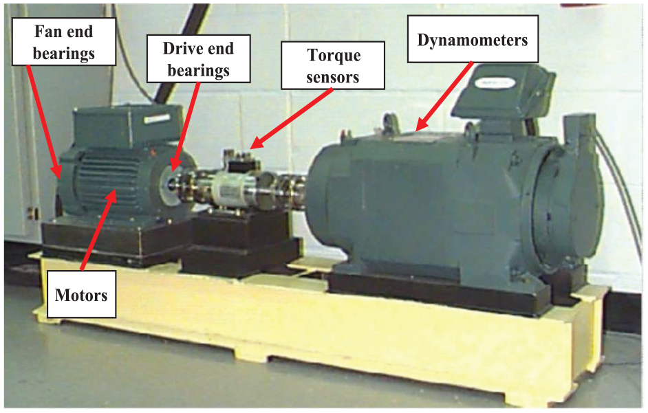
Case western reserve university bearing experimental platform.

Figure 8.

The single point of failure bearing diagram: (a) Outer ring fault. (b) Inner ring fault. (c) Ball body fault. (d) A combination of faults.

The vibration data of different ball-body fault-size bearings at the drive end were used for the few-shot variable working condition fault diagnosis experiment at a data sampling frequency of 12 KHz, using 100 data samples under each load and fault size. The specific few-shot variable working condition bearing fault data set is shown in Table 1.

Table 1.

The data set of four types of faulty bearings under variable loads.

Fault type	Load (hp)	Fault size (inch)	Fault location	Number of samples
Normal bearing	0–3	0	\	100
Inner ring failure	0–3	0.007, 0.014, 0.021, 0.028	\	100
Ball body failure	0–3	0.007, 0.014, 0.021, 0.028	\	100
Outer ring failure	0–3	0.007, 0.014, 0.021, 0.028	6 o’clock	100

Results and discussion

Fault diagnosis of the bearings with different fault sizes under the same load

To verify the diagnostic efficacy of the proposed EMRN model for few-shot bearing faults of different fault sizes, the training and test sets selected from Table 1 are shown in Table 2. The data sets all contain four types of bearing faults, with 100 samples for each type. Furthermore, 4-way 1-shot (4W1S), 4-way 5-shot (4W5S), and 4-way 10-shot (4W10S) experimental sets were established. Five experiments were conducted for each set, and the results were expressed as the average value of the five tests.

Table 2.

The experimental diagnostic data division of bearing faults of different sizes.

Dataset	Load	Fault type	Fault size (inch)	Sample size
Training set	0 hp	Normal bearing Inner ring failure Ball body failure Outer ring failure	0.007	Fault samples for each fault level in each category of operating conditions are 100
Test set	0 hp		0.014

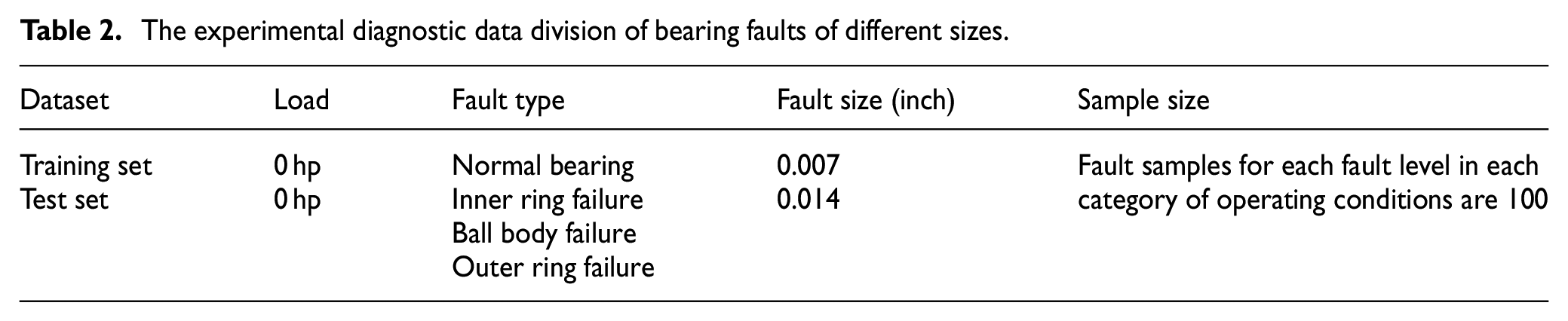
To demonstrate the diagnostic performance of the EMRN model more intuitively, in addition to comparing it with the diagnostic effect of the RN, a few-shot bearing fault diagnosis comparison experiment was conducted in the same experimental conditions using Matching Net, a few-shot MLFD method. The experimental comparison results between the 4W1S, 4W5S, and 4W10S samples are shown successively in Figure 9.

Figure 9.

A test accuracy comparison of different fault diagnosis methods at different fault sizes.

As illustrated in Figure 9, the EMRN model proposed in this paper was more successful in diagnosing faults in all three experimental groups than the other two few-shot MLFD methods. This indicated that introducing EEMD into the RN to decompose and stitch the original faults after STFT further highlighted the fault features. This allowed the subsequent embedding modules in the RN to extract more precise fault features while improving the fault diagnosis accuracy. Furthermore, when the number of fault categories (way) was certain, the diagnostic accuracy of all three fault diagnosis methods improved as the number of fault samples increased (shot). This indicated that model overfitting was reduced as the number of samples increased, improving its diagnostic accuracy. Although the diagnostic accuracy of all three methods improved in the 4W1S and 4W5S experimental groups, that of EMRN was higher than the matching network (MN) and RN. Specifically, the diagnostic accuracy of MN and RN increased by 7.4% and 8.78%, respectively, as the shot number increased from 1 to 5, denoting a growth in both of less than 10%. Contrarily, the diagnostic accuracy of EMRN increased by as much as 11.08%. In the 4W10S experimental group, the diagnostic accuracy of all three fault diagnosis methods exceeded 90%, of which that of EMRN was as high as 94.56%, which was 2.14% and 1.32% higher than that of MN and RN, respectively. Overall, with a few-shot fault size, the proposed fault diagnosis model performed better in identifying different sizes and types of bearing faults, highlighting its efficacy.

In order to verify the robustness of the model under different signal processing schemes, corresponding comparative experiments were carried out. Replace the sample of the previous experimental test set with a sample of 0.021 in, and the other conditions remain unchanged. Figure 10 shows the accuracy results of fault diagnosis experiments between the proposed method and the method after EMD and VMD processing.

Figure 10.

Test accuracy of different signal processing methods.

As can be seen from Figure 10, the results show that the accuracy of eemd and vmd signal decomposition is higher than that of emd based method. Because eemd and vmd overcome the problems of end effect and mode component aliasing in EMD methods, they are suitable for non-stationary sequences. However, the mode number K is required to be defined in advance in vmd, and the value of K has a certain influence on the decomposition result. For example, the optimization of K value has a problem of large computation. Therefore, this paper chooses the eemd decomposition method.

Bearing fault diagnosis under variable loads

Bearing fault diagnosis experiments under variable load were conducted to verify the generalization performance of the proposed model. The corresponding experimental data sets selected from Table 1 were divided into experimental data, as shown in Table 3. The experiments were divided into experiments A, B, and C. Each experiment included 4W1S, 4W5S, and 4W10S groups, while the rest of the experimental settings were consistent with Section 3.2.1. The experimental results are shown in Figure 11.

Table 3.

The experimental data division of bearing fault diagnosis under variable loads.

	Dataset	Load	Fault type	Fault size (inch)	Sample size
A	Training set	0 hp	Normal bearing Inner ring failure Ball body failure Outer ring failure	0.007	Fault samples for each fault level in each category of operating conditions are 100
	Test set	1 hp
B	Training set	0 hp
	Test set	2 hp
C	Training set	0 hp
	Test set	3 hp

Figure 11.

The experimental results of the bearing fault diagnosis under variable loads.

As shown in Figure 11, the proposed model performed well in the three variable-load bearing fault diagnosis experiments. The diagnostic accuracy of the model reached >65% in experiments A, B, and C in the 4W1S experimental group and rose as the number of samples (shot) increased. This was consistent with the law of the few-shot MLFD method, that is, the diagnostic accuracy of the fault diagnosis model rose as the number of sample shots increased in each category. At a shot number of 10, the diagnostic accuracy of the model exceeded 86.24% in all cases, especially in experiment A, showing a diagnostic accuracy of as high as 91.3%. However, a comparison between the fault diagnosis results of experiments A, B, and C at the same number of ways and shots showed that the diagnostic accuracy of the model did not improve as the load of the test set increased and that of the training set was certain (a load of 0 hp). In 4W5S, the diagnostic accuracy of experiment A was 79.2%, while that of experiments B and C were lower by 0.4% and 3.8%, respectively. This indicated that the proposed model displayed good diagnostic results and generalization performance under variable loads.

Fault diagnosis for different fault size bearings under variable loads

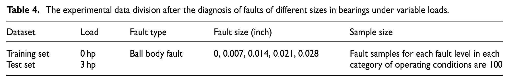
To verify the effectiveness of the proposed EMRN model in fault diagnosis of bearings with different fault sizes under variable load, the data of bearings with different fault sizes under ball body fault were selected for experiments. The experimental data are divided as shown in Table 4. The 5-way 1-shot (5W1S), 5-way 5-shot (5W5S), and 5-way 10-shot (5W10S) experimental groups were established, while the rest of the experimental settings were kept consistent with Section 3.2.1.

Table 4.

The experimental data division after the diagnosis of faults of different sizes in bearings under variable loads.

Dataset	Load	Fault type	Fault size (inch)	Sample size
Training set	0 hp	Ball body fault	0, 0.007, 0.014, 0.021, 0.028	Fault samples for each fault level in each category of operating conditions are 100
Test set	3 hp

To verify the diagnostic performance of the EMRN model, comparative fault diagnosis experiments were conducted using the MN and RN few-shot MLFD methods with the same data set. The experimental results showed that the diagnostic effect of the EMRN model varied in the different experimental groups, as shown in Figure 12.

Figure 12.

The experimental results of the fault diagnosis in bearings with different fault sizes under variable loads.

As shown in Figure 12, the fault diagnosis accuracy of the MN, RN, and EMRN improved as the number of samples (shot) increased. In the 5W1S experimental group, the EMRN model performed better than the other two methods, with a diagnostic accuracy reaching 83.16%, while that of MN and RN was only 69.24% and 69%, respectively. At a sample number (shot) of 10, the diagnostic accuracy of all three fault diagnosis methods exceeded 90%, with that of the proposed model at 95.2%, which was 4.0 percentage points higher than the MN method. Constructing the original signal via decomposing, STFT transformation, and splicing effectively improved the randomness and blindness of the convolutional operation and enhanced the accuracy of fault feature extraction in the RN, consequently increasing the overall diagnostic performance. Therefore, the proposed EMRN model effectively diagnosed the ball-bearing dataset with different fault levels under variable loads, displaying better fault diagnosis performance in few-shot variable load ball-bearing fault experiments.

Conclusion

Bearing fault diagnosis methods present challenges, such as a small number of bearing fault samples and substantial differences in bearing operating conditions, leading to poor model generalization performance and low diagnostic accuracy. This paper proposes a few-shot fault method for bearing fault diagnosis based on EEMD and RN (EMRN). The results are as follows:

• a) A few-shot meta-learning RN is used for bearing fault diagnosis. The RN improves the generalization ability of the model by learning the interrelationships between samples, enhancing its diagnostic accuracy for few-shot-size bearing faults.

• b) The EEMD module is introduced into the RN to construct multi-dimensional fault features for the original fault signal. Original signal decomposition, STFT transformation, and splicing effectively improve challenges, such as the randomness and blindness of the convolutional operation, and enhance the accuracy of the subsequent fault feature extraction in the RN, consequently increasing the overall diagnostic performance of the model.

• c) In the few-shot variable-load bearing fault diagnosis experiments, the proposed model shows significantly higher diagnostic accuracy and excellent generalization performance than the MN and RN models in the meta-learning approach, the accuracy of the model remained above 80% in 5way-Nshot experiments. In particular, the diagnostic accuracy of the proposed model improves significantly in the 5W10S experimental group, reached 95.2% accuracy, involving different fault sizes at the same fault type of variable loads.

In the future, this paper will continue to improve the model, and carry out gear and bearing fault diagnosis experiments, and strive to improve the fault diagnosis accuracy of the model in the aspects of cross-equipment and cross-parts.