Sage Journals: Discover world-class research

Abstract

Nowadays, when it comes to bearing faults monitoring, several solutions and implementations are in vogue due to the interest they arouse. It can be seen both in the types of hardware solutions used and, in the signal-processing algorithms and techniques employed. However, for a fault such as the bearing fault, which accounts for 41% of all faults in these systems and is also the source of the majority of other faults, it appears that the approaches used until now are insufficient for containing this fault and the losses it generates. The aim of this work is to present a new system dedicated exclusively to bearings, while also conducting a comparative study of the various algorithms currently used for mechanical fault detection, based on the mathematical model of the stator current signal used in the MCSA method, which is very close to the induced current signal. At the end, results of all simulations demonstrated that, in addition to the ESPRIT-TLS method, which is currently the best in terms of accuracy, the Varpro method could be a promising alternative.

Keywords

Electromechanical faults bearing fault high resolution signal processing algorithm mode decomposition algorithm variables projection algorithm

Introduction

Today, the use of electromechanical machines in many areas has made their monitoring a matter of great importance. This is due to the significant damage that can be caused by failures of their mechanical and electrical components. However, of all these components, the bearing is the one that causes the most losses.^1,2 It accounts for 41% of all faults occurring in these systems.^3–6 Several signal acquisition techniques have been used for decades. The most widely used for online monitoring are the technique based on vibration and electrical sensors.^7–10 The big problem is that these techniques have considerable limitations in terms of developing an accurate, real-time system. In the case of the vibration analysis technique, the biggest problem is that the vibration sensors capture all vibrations around the component where they are placed. In other words, in addition to the vibration caused by the appearance and evolution of the fault, they also sense all the surrounding vibrations and noises. It means that, when analysing the signal, it is necessary to go through several processes to retain useful signal. Also, because of others vibrations, this can lead to errors in detection and decision-making. So, what’s the point in taking a lot of time to laminate the signal and end up with useless information, without mentioning the fact that during the time it takes to decide whether the fault is present or not, not only may the fault appear, but it may also have taken significant proportions.¹¹ On the other hand, a potential drawback of the approach based on stator current analysis is that it includes the participation of all other faults that may occur in the machine in addition to the fault being investigated. As a result, the signal captured is a combination of all other potential fault signals, including those originating from the bearing fault.^12–14 So, in this situation, signal decomposition becomes the first thing to do. Then comes the identification of the bearing fault. It can be time-consuming and distort the real-time nature of detection. Coming to the signal processing techniques combined with them, methods such as fast Fourier transform FFT,^15,16 STFT,^17,18 WVD,^19–22 wavelet analysis was the first to be used. But because of their limitations, such as poor signal comprehension, a frequency resolution problem, a limited number of analysis points for FFT; a fixed windowing size, poor simultaneous frequency and temporal resolution for the STFT and the WVD, and the failure to decompose the signal into its elementary signals for the WT, they have pushed researchers to explore new methods. This is where algorithms such as EMD and VMD^23–25 become relevant for the proper decomposition of the composite signal, as well as algorithms capable of extracting essential signal characteristics such as frequencies and amplitudes. These techniques include ESPRIT,^26,27 SAGE,^28–30 CLEAN^31,32 and Varpro.^33–35 From this panoply of literature, it is clear that techniques and methods exist in large numbers. However, making the right choice requires evaluating them based on some metrics such as computation time or complexity, detection accuracy, and sometimes memory space. It is evident that the old acquisition techniques are inadequate for detecting only bearing faults. This means no improvement in detection performance side, but also a side of designing appropriate systems.

The main objective of this work is to present this new system dedicated exclusively to the monitoring of bearing defects but also to compare the latest signal processing algorithms used in the detection of defects in electromechanical systems such as variable projection (VarPro), SAGE, Clean, mode decomposition algorithm (EMD, VMD), and ESPRIT-TLS for the detection of mechanical bearings only.

This work is performed as follows,

First, we give a brief overview of the bearing defect. Then we present the proposed system for the detection of bearing fault only. Next, we provide an overview of these algorithms. Finally, after presenting the simulation and the results obtained using MATLAB software, we conclude with the conclusion and future perspectives.

Bearing fault modelling and detection

In the literature, the major causes of rotating machine failures are faults caused by fatigue spalling, lubricant contamination, excessive load, or other causes or electrical causes.^36,37 Faults in bearings are based on several effects in rotating machines, namely, an increase in the noise level and the appearance of vibrations owing to the rotor’s movements around the longitudinal axis of the machine.³⁶ This type of fault also causes variations (oscillations) in the torque of the machine load, thereby blocking the rotor. It should also be mentioned that bearings with balls are composed of two rings, internal ring and external ring between which there are several balls or rotating rollers. When the bearing is operating under normal conditions, the fatigue defect starts with small cracks under the raceway and rolling element surfaces, and progressively spreads over the contact surface, increasing the number of harmonics over time.³⁸ In addition, bearing faults are most often related to eccentricity faults, which induce rotor asymmetry. These bearing defects occur most often when the inner or outer surfaces of the inner or outer ring are affected by damage or ball defects.³⁶ In addition, because the axis that links the rotor axis and load-bearing axis passes through the centre of the bearing, any defect within the bearing will directly affect this axis. Thus, the system placed on the axis underwent the same sudden changes, generating a variation in the received flux.³⁹ In Figure 1, we show what a bearing looks like and its various faults. The expression that gives the characteristic frequencies of the bearing fault is as follows:

f_{bng} = | f_{0} \pm k f_{i, o} |

(1)

where

k = 1, …, N

and

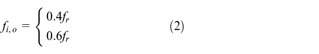
f_{i, o} = {\begin{matrix} 0.4 f_{r} \\ 0.6 f_{r} \end{matrix}

(2)

where $f_{0}$ is the supply frequency, $k$ the factor relies on harmonic numbers, $f_{i, o}$ the frequency of damage relies on the inner or outer raceway and $f_{r}$ is the rotor pulsation frequency.

Figure 1.

Bearing fault. (a) Ball fault, (b) inner ring fault, (c) outer ring fault, (d) cage fault.

Presentation of the system used

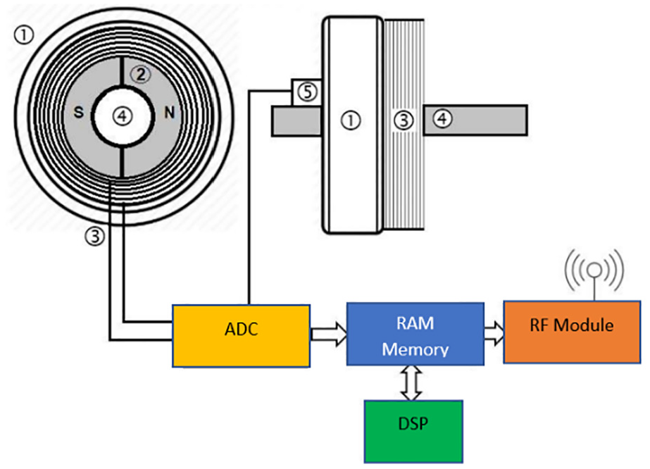
The system proposed in this work for detecting only bearing faults exploits the principle of the induced current created by the variation of the magnetic flux through a copper coil. Thus, a sensor connected to the end of these coils captures this induced current and a vibration sensor placed on bearing axis captures all other variations. This is the case when the bearing carrying the magnets is defective. Once acquired, this induced current is used by algorithms embedded on the DSP card to extract the parameters that can then determine whether the bearing is in good condition or not through artificial intelligence algorithms. This intelligent algorithms can be deployed locally or online in a cloud as show on Figure 2. The main parts of this system are as follows: the bearing with the two magnet poles placed on internal ring, the copper coil placed on external ring that allows to receive the variations of the magnetic flux according to the state of the bearing, the analog-digital converter for the acquisition and conversion of the signal, the DSP card or processing unit, and the RF module for the transmission of the data online.

Figure 2.

Architecture of monitoring system.

Modelling of the perceived system signal

The signal model used in this study has the same nature as the stator signal used in the MCSA method and its variants. The principle of this method is the analysis of the current to detect the presence of a possible anomaly in the entire machine or one of its components. However, the difference with the system shown in Figure 3 is that the signal is not captured from the electrical line coming from the stator, but only from the interaction (magnet field) between the movement of the magnets and copper coil on the bearing, which not allows any other fault detection. And this avoid to have a detction system that may be too costly for the development of a real-time monitoring system. Thus, knowing the characteristics of a bearing fault that can manifest itself by the appearance of special harmonics in the normal signal (signal composed only of the frequency $f_{0}$ ), and because the induced current signal is very close to the signal of stator current, the signal captured from the new system can be expressed as follows⁴⁰:

s [n] = \sum_{k = - L}^{L} a_{k} \cos (2 π f_{k} \times n / F_{k} + Φ_{k}) + w [n]

(3)

Where s[n] denotes a sample of the signal at time n, w[n] the additive Gaussian noise at time n, L the exact sinusoidal number contained in the signal, f_k are the frequencies of bearing fault, a_k the amplitudes and Φ_k the phase of fault’s harmonics contained in the n-th sample.

Figure 3.

Fault detection procedure.

Determining the number of harmonics in the fault signal

The methods presented in this work require prior knowledge of the number of harmonics containing inside the signal to be analysed to extract parameters such as frequencies and amplitudes. Techniques for doing this are known as Model Order Selection (MOS). These methods, based on the retention of essential information from a signal, enable us to know the number of parameters to be analysed in advance. These include the AIC, MDL, FPE, KIC, and RAE.⁴¹ This is the first step in all the parametric methods. In the simulation and results section, we present how MDL and AIC are applied to determine the number of harmonics in the bearing fault signal at low and high amplitudes for certain SNR values.

Overview of the fives algorithm used

EMD method

Similar to Fourier decomposition, the empirical mode decomposition (EMD) algorithm decomposes a given signal into an elementary sum of signals and a residual. The method was introduced by Huang et al.^23,42–44 The mathematical expression is as follows:

x [n] = \sum_{k = 1}^{n} M_{k} (m) + R_{n} (m)

(4)

where $M_{k} (m)$ denotes the k-th empirical mode at time n, and $R_{n} (m)$ is the residual after the extraction of the empirical modes. The intrinsic mode function (IMF) is the name given to each. However, to be so, any mode must meet two²³ criteria: (1) it must be made up of an equal number of local maximums and zero crossings or must be different by one unit in number; (2) the average of the envelope that precedes it and the one that follows it must be zero at all points. The extraction process called sifting process²⁴ is the following:

For a sample at time n of the signal X,

Take the maxima and minima

draw the lower and upper envelopes

Calculate the average of these two envelopes

Subtract the average of the time series of the sample as follows

Verify conditions for stopping the extraction of modes:

SC = \sum (prev (H) - H)^{2} / prev {(H)}^{2}

(5)

Repeat the instructions from 1 to 5 as long as SC < 0.3.

After obtaining the modes, the last step is to determine the frequency representations to extract the frequencies.

VMD method

Similar to EMD, the Variational Mode Decomposition (VMD) algorithm finds all the series that make up a given signal.^45,46 Unlike EMD, with VMD, the spectral bandwidth of each mode is chosen as the extraction unit. In other words, VMD assumes that each mode is fixed around a central frequency, which must be determined during the same decomposition period.^47,48 The following steps must be taken to determine the bandwidth of a mode: (1) Exploit the Hilbert transform to compute the analytical signal of each mode; (2) Each mode was shifted to its ‘baseband’ using an exponential factor; (3) Estimate the bandwidth.²³ The algorithm used by VMD to decompose the signal is called the Alternating Direction Method of Multipliers. The detailed structure of this algorithm can be found in Reference²⁵.

ESPRIT-TLS

The ESPRIT-TLS algorithm is the most robust and accurate variant of the ESPRIT high-resolution signal processing algorithm. Unlike others, the TLS algorithm is used to estimate the parameters of a given signal. ESPRIT is one of the signal processing algorithms that, starting from a given signal, subdivides it into two spaces called signal and noise in order to extract characteristics such as the amplitudes and frequencies of each harmonic present that compose it.^26,27,49,50 It is used in the resolution of TLS problems.⁵¹ It is based on the decomposition using SVD.^52,53 The work in Reference ⁵⁴ provides a more detailed understanding of the use cases of the TLS algorithm. Its combination with ESPRIT can be found in the following publication.⁵⁵

CLEAN method

This algorithm, exploiting the principle of deconvolution over several iterations of the spectral band of the signal domain, allows the estimation of the signal parameters of most so-called nonlinear square (NLS) problems. It is largely used for situations where several pieces of data are missing to clarify the signal, as well as when the signal is strongly affected by noise, as in geoscience and astrophysical science.^31,32,56,57 This algorithm is very robust, easy to implement, and manages to filter the signal from the additive noise that composes it to allow a better estimation of these parameters. The structure of the algorithm was described in the following reference.³¹

SAGE method

This algorithm, which spares signals in single harmonics by eliminating the interference that may exist between them based on interference cancellation to separate any signal into harmonics in the so-called waiting stage (expectation step), is an improvement of the EM algorithm.⁵⁸ Using the maximum likelihood principle,⁵⁹ the cost function was optimized to extract the required parameters. Instead of using the usual EM algorithm process, the optimization is performed using two unidimensional optimization procedures in series.^28–30 To initialize the parameters before starting the optimization process, the algorithm uses a Fourier transform-based frequency parameter estimation and serial separation of the given signal. By updating the searched parameters sequentially, the algorithm alternates between several small data spaces defined by the designer. This algorithm is commonly used in the telecom domain to determine the direction of arrival of signals on a receiver. Over time, it has been adapted to composite signals of the same nature as the mathematical model presented in equation (3). The detailed structure of the SAGE algorithm can be found in this study.⁵⁸

Variables projection method

To analyse a signal from its parameters, parametric methods are most often used. These methods are then satisfied by predicting an almost perfect model that allows obtaining the desired signal to model the observed signal. This was achieved by determining these parameters according to a fixed error threshold.^{33–35,60,61} This is sometimes referred to as the minimization of a cost function. This is what Golub and Pereyra did in their 1973 work, where they showed how to solve most of the so-called separable nonlinear least squares problem (SNLLS) using an algorithm called variable projection (VarPro). Moreover, what is interesting with their work is that they showed that for any problem of estimation of more than two frequencies, that this problem could be considered as an SNLLS problem.^62,63 The structure of this algorithm can be found in this work by Dianne P. O’Leary-Bert W. Rust.³⁵ The key steps are as follows.

Solving Constrained Nonlinear Least-Squares Problems

Solving Constrained Linear Least-Squares Problems using Matlab’s lsqlin function

Computing the Jacobian Matrix of the cost function and how to use it along the algorithm.

Results of simulation

Simulation’s parameters

In our present study, the parameters used for the simulation part and the results obtained are presented in Table 1 below. These parameters are used in the mathematical model of the signal presented in equation (3) to obtain the signal to be analysed. For the amplitudes, we used different values for the small and large ones. The small ones were obtained by dividing the large ones by 10, as shown in Table 2. The frequencies of the defect are obtained from the mathematical model and the value of k, which is the factor determining the number of harmonics of the defect in addition to the fundamental frequency. As mentioned above, MDL and AIC were applied to three, five, and seven harmonics to extract the number of harmonics that is not known a priori in the estimation of the actual parameters. The value on the n-axis corresponding to the minimum cost function is the number of harmonics constituting the observed signal. The following figures provide an overview of the results.

Table 1.

Simulation parameters.

Parameters	Value
$f_{r}$	29.01 Hz
$f_{0}$	50 Hz
$n_{b}$	12
$f_{i, o}$	139.248 Hz
$F_{s}$	1000 Hz
$k$	1,2,3
$SNR$	[0–51] dB
$Processor$	Intel Pentium(R) CPU B950 @ 2.1 GHz× 2

Table 2.

Amplitudes and frequencies used for simulation.

Harmonics’s number	Amplitudes (A)	Frequencies (Hz)	Amplitudes a₀ (A)	Frequencie $f_{0}$ (Hz)
3	[10 0.6 0.4]	[89.248 189.248]	10	50
5	[7 4 3 2 5]	[89.248 189.248 228.4960 328.4960]	7
7	[7 5 3 4 5 6 7]	[89.248 189.248 228.4960 328.4960 367.7440 467.7440]	7

From Figures 4 and 5, it is clear that of the two algorithms, the MDL algorithm is the one that best estimates the number of harmonics composing the signal. However, it can be seen that when noise dominates, whether at low or high amplitude, the estimated number of n frequencies of the signals is different from the exact NH value of the signal. In addition, this parameter is very well estimated when there is less noise. Therefore, we deduce that noise is an important factor to reduce for the correct estimation of the number of harmonics. Otherwise, even in the presence of a defect, the system designed would indicate the absence of any defect, and by the time it realizes that it has a defect, the severity will have already changed enormously.

Figure 4.

Estimation of Harmonics number NH with is n for large amplitudes for SNR = [−5 10 50] dB.

Figure 5.

Estimation of Harmonics number NH with is n for small amplitudes for SNR = [−5 10 50] dB.

Simulation results

This part gives an overview of the results of the simulation performed with these six algorithms in the estimation of the frequency harmonics of the rolling defect contained in the signal synthesized in equation (3). We use the NMSE (Normalized mean square error) to measure the accuracies of this estimate for Nh equal to two, four and six harmonics of the bearing fault. But before presenting these results, we give in Figure 6 the representations of the signal in the frequency domain according to each number of harmonics.

Figure 6.

Frequency domain representation of the signal. (a) Nh = 2, (b) Nh = 4 and (c) Nh = 6.

Simulation results for two harmonics

For large amplitudes

For small amplitudes

Simulation results for four harmonics

For large amplitudes

For small amplitudes

Simulation results for 6 harmonics

For large amplitudes

For small amplitudes

Discussions

Based on the above results (from Figures 7 to 12), the VMD, SAGE, ESPRIT-TLS, and VarPro algorithms can be selected in estimating the frequency of the bearing defect for accuracy. However, given the ‘real-time’ aspect, SAGE and VMD are time-consuming even though their memory sizes are minimal compared to TLS and VarPro. However, since the memory space of the latter two is on the order of a few KB, they can be perfect candidates for a real-time estimation of small memory sizes.

Figure 7.

Simulation for two harmonics with large amplitudes. (a) mean of NMSE on f₁f₂f₃ estimation, (b) average execution time of each algorithm, (c) memory size of each algorithm.

Figure 8.

Simulation for two harmonics with small amplitudes. (a) mean of NMSE on f₁f₂f₃ estimation, (b) average execution time of each algorithm, (c) memory size of each algorithm.

Figure 9.

Simulation for 4 harmonics with large amplitudes. (a) Mean of NMSE on f₁f₂f₃f₄f₅ estimation, (b) Average execution time of each algorithm, (c) Memory size of each algorithm.

Figure 10.

Simulation for four harmonics with small amplitudes. (a) mean of NMSE on f₁f₂f₃f₄f₅ estimation, (b) average execution time of each algorithm, (c) memory size of each algorithm.

Figure 11.

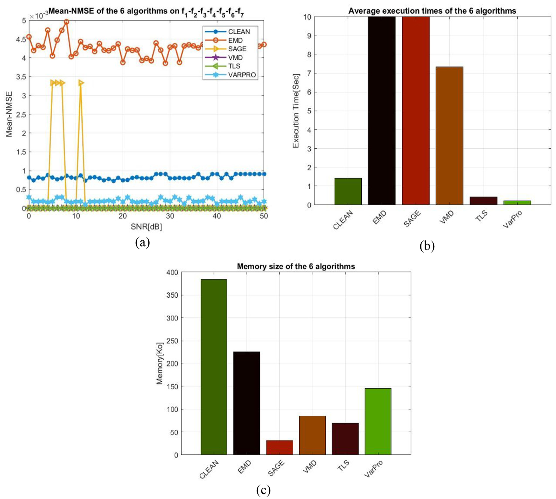
Simulation for six harmonics with large amplitudes. (a) mean of NMSE on f₁f₂f₃f₄f₅f₆f₇ estimation, (b) average execution time of each algorithm, (c) memory size of each algorithm.

Figure 12.

Simulation for four harmonics with small amplitudes. (a) Mean of NMSE on f₁f₂f₃f₄f₅f₆f₇ estimation, (b) average execution time of each algorithm, (c) memory size of each algorithm.

The last thing to analyse is the behaviour of these two for very close frequencies with $f_{1} = 50 Hz, f_{2}$ =51 Hz and $f_{2} = 52 Hz$ . For this purpose, we limit ourselves to two harmonics at this point to conclude with $a_{1} = 10 A, a_{2} = 0.6 A and a_{2} = 0.4 A$ .

In addition, it is clear from Figure 13 that the ESPRIT-TLS algorithm outperforms all others, including Varpro, in estimating the frequencies of the single bearing fault. As far as Varpro is concerned, he needs to have knowledge of the signal model for the estimation process. In addition, not only does it use a notion of weight that must be well chosen, but also the choice of the initial values of the parameters can influence the estimate. However, with ESPRIT-TLS, even without knowing the signal model, it is possible to estimate the frequencies and amplitudes of the elementary signals contained in the signal by knowing only the number of harmonics estimable by the MOS method. This is also the case for the signal of rotating machines, where it is impossible to know in advance the pattern of the signal. This makes it a much more perfect choice than Varpro, although for the latter, a good choice of weights and a good initialization led to good estimates.

Figure 13.

Simulation for close harmonics with small amplitudes. (a) Mean of NMSE on f₁f₂f₃ estimation, (b) zoom on Mean of NMSE on f₁f₂f₃.

Conclusion et perspectives

In view of these results, taking into account the size of the memory, in particular the accuracy in the estimation of the signal parameters for the correct detection of the bearing fault and the real-time character of the system, we can finally come to the end of this work by saying that the Varpro algorithm could have been a good choice. But due to conditions such as my knowledge of the observed signal pattern and the right choice of parameters, ESPRIT-TLS is much better not only in terms of accuracy but also in terms of simplicity. So, in conclusion, ESPRIT-TLS would be a good choice among all the algorithms to explore for bearing defect detection alone. However, as these results are experimental, we wish to continue this work by moving to a test bench with the proposed system mounted with defective bearings, in order to confirm the conclusion reached in this study of the analysis and comparison of these six algorithms. Since this work is only the beginning of a series of works, we intend to subsequently perform a comparison of the techniques present in this work and other techniques from the emerging fields of signal processing for fault diagnosis in various industrial applications, in particular in terms of the fault information-guided variational mode decomposition (FIVMD) method for the diagnosis of rolling element bearings, the Vold-Kalman filter bandwidth selection scheme based on the order spectrum for the diagnosis of gearbox faults in offshore wind turbines, and the new vibration-based prognostic scheme for managing the condition of gears in surface wear the evolution of the intelligent manufacturing system. In addition, because of the errors that can be made in the estimation of the number of harmonics even for the ESPRIT-TLS algorithm, we plan to look for another method that does not exploit this parameter in one of the next works.

Footnotes

Handling Editor: Aarthy Esakkiappan

Authors’ contributions

Pascal Dore: student Ph.D, producer of this work (contact the corresponding author).

Pr Saad Chakkor, Supervisor of this work.

Pr Ahmed El Oualkadi, Director of thesis.

Mostafa Baghouri Co-supervisor.

Declaration of conflicting interests

The author(s) declared no potential conflicts of interest with respect to the research, authorship, and/or publication of this article.

Funding

The author(s) received no financial support for the research, authorship, and/or publication of this article.

Ethics approval

Not applicable.

Consent to participate

We, authors of this paper consent to participate to the publication of this paper.

Consent for publication

All authors consent for publication.

ORCID iD

Pascal Dore

Availability of data and material

Regarding the data used, they can be obtained from the mathematical model of the stator signal used for this purpose (see equation 3, 1 and 2) and the parameters specified in Tables 1 and 2.

Code availability

Codes are available on demand. The Persons can contact the corresponding author.

References

Raison

Rostaing

Butscher

, et al. Investigations of algorithms for bearing fault detection in induction drives. In: Proc. IEEE 28th annual conference of the Industrial Electronics Society, Sevilla, Spain, 2002, vol. 2, pp. 1696–1701.

Guyer

. Rolling Bearings Handbook and Troubleshooting Guide. Radnor, Pennsylvania: Chilton Book Compagny, 1996.

Bonnett

Yung

. Increased efficiency versus increased reliability. IEEE Ind Appl Mag 2008; 14: 29–36.

Thorsen

Dalva

. A survey of faults on induction motors in offshore oil industry, petrochemical industry, gas terminals, and oil refineries. IEEE Trans Ind Appl 1995; 31: 1186–1196.

Thomson

. A review of on-line condition monitoring techniques for three-phase squirrelcage induction motors–past, present and future. In: 2nd IEEE international symposium on diagnostics for electrical machines, power electronics and drives—SDEMPED ‘99, Gijon, Spain, 1999, pp. 3-17.

Thorsen

Dalva

. Failure identification and analysis for high-voltage induction motors in the petrochemical industry. IEEE Trans Ind Appl 1999; 35: 810–818.

Zarei

Tajeddini

Karimi

. Vibration analysis for bearing fault detection and classification using an intelligent filter. Mechatronics 2014; 24: 151–157.

Plante

Nejadpak

Yang

. Vibration analysis: fault detection and failure prediction. In Proc. IEEE AUTOTESTCON, 2015.

El Bouharrouti

Morinigo-Sotelo

Belahcen

. Multi-rate vibration signal analysis for bearing fault detection in induction machines using supervised learning classifiers. Machines 2023; 12: 17.

10.

Zhou

Habetler

Harley

. Stator current-based bearing fault detection techniques: a general review. In: 2007 IEEE international symposium on diagnostics for electric machines, power electronics and drives, Cracow, Poland, 2007, pp. 7–10. DOI: 10.1109/DEMPED.2007.4393063.

11.

Wang

Yang

, et al. A model-based method for bearing fault detection using motor current. J Phys Conf Ser 2020; 1650.

12.

Trajin

. Détection automatique et diagnostic des défauts de roulements dans une machine asynchrone par analyse spectrale des courants statoriques. In: Conférences des jeunes chercheurs en Génie électrique, December 2008, Lyon, France.

13.

Singh

Kumar

. Motor current signature analysis for bearing fault detection in mechanical systems. Procedia Mater Sci 2014; 6: 171–177.

14.

Morales-Perez

Grande-Barreto

Rangel-Magdaleno

, et al. Bearing fault detection in induction motors using MCSA and statistical analysis. In: 2018 IEEE international instrumentation and measurement technology conference (I2MTC), Houston, TX, USA, 2018, pp. 1-5. DOI: 10.1109/I2MTC.2018.8409780.

15.

Zhou

Qin

Kou

, et al. Fault detection of rolling bearing based on FFT and classification. J Adv Mech Des Syst Manuf 2015; 9: JAMDSM0056–JAMDSM0056.

16.

Rai

Mohanty

. Bearing fault diagnosis using FFT of intrinsic mode functions in Hilbert–Huang transform. Mech Syst Signal Process 2007; 21: 2607–2615.

17.

Cocconcelli

Zimroz

Rubini

, et al. STFT based approach for ball bearing fault detection in a varying speed motor. In: Fakhfakh

Bartelmus

Chaari

, et al. (eds) Condition Monitoring of machinery in Non-Stationary operations. Berlin, Heidelberg: Springer, 2012.

18.

Liu

Cheng

Wen

. Rolling bearing fault diagnosis via STFT and improved instantaneous frequency estimation method. Procedia Manuf 2020; 49: 166–172.

19.

Quinde

Sumba

Ochoa

, et al. Bearing fault diagnosis based on optimal time-frequency representation method. IFAC-PapersOnLine 2019; 52: 194–199.

20.

Meng

. Rotating machinery fault diagnosis using Wigner distribution. Mech Syst Signal Process 1991; 5: 155–166.

21.

Singru

Krishnakumar

Natarajan

, et al. Bearing failure prediction using Wigner-Ville distribution, modified poincare mapping and fast Fourier transform. J Vibroengineering 2018; 20: 127–137.

22.

Cai

Chen

. Bearing Fault diagnosis method based on local mean decomposition and Wigner higher moment spectrum. Exp Tech 2016; 40: 1437–1446.

23.

Huang

Shen

Long

, et al. The empirical mode decomposition and the Hilbert spectrum for nonlinear and non-stationary time series analysis. Proc Royal Soc London, Ser A – Math, Phys Eng Sci 1998; 454: 903–995.

24.

Dybała

Zimroz

. Rolling bearing diagnosing method based on empirical mode decomposition of machine vibration signal. Appl Acoust 2014; 77: 195–203.

25.

Mohanty

Gupta

Raju

. Comparative study between VMD and EMD in bearing fault diagnosis. In: 2014 9th International conference on industrial and information systems (ICIIS), pp. 1–6. DOI: 10.1109/ICIINFS.2014.7036515.

26.

These_saad Saad Chakkor. E-diagnostic de processus physiques à base des méthodes de haute résolution Application: machines éoliennes. Instrumentations et Détecteurs [physics.ins-det]. Faculté des Sciences de Tétouan, Maroc, 2015.

27.

Agrawal

Mohanty

Agarwal

. Bearing fault detection using Hilbert and high frequency resolution techniques. IETE J Res 2015; 61: 99–108.

28.

Fleury

Dahlhaus

Heddergott

, et al. Wideband angle of arrival estimation using the Sage algorithm,. In: Proc. IEEE fourth Int. Symp. spread spectrum techniques and applications (ISSSTA ’96), Mainz, Germany, Sept. 1996, pp. 79–85.

29.

Tschudin

Heddergott

Truffer

. Validation of a high resolution measurement technique for estimating the parameters of impinging waves in indoor environments. In: Proc. 9th IEEE Int. Symp. personal, indoor and mobile radio communications (PIMRC ’98), Boston, MA, September 1998, pp. 1411–1416.

30.

Fessler

Hero

. Space-alternating generalized expectation-maximization algorithm. IEEE Trans Signal Process 1994; 42: 2664–2677.

31.

Baisch

Bokelmann

GHR

. Spectral analysis with incomplete time series: an example from seismology. Comput Geosci 1999; 25: 739–750.

32.

Kong

Han

Wei

. Modified gradient algorithm for total least square filtering. Neurocomputing 2006; 70: 568–576.

33.

Golub

Pereyra

. The differentiation of pseudo-inverses and nonlinear least squares problems whose variables separate. SIAM J Numer Anal 1973; 10: 413–432.

34.

Kaufman

. A variable projection method for solving separable nonlinear least squares problems. DAIMI Rep Ser 1974; 3. DOI: 10.7146/dpb.v3i27.6446

35.

O’Leary

Rust

. Variable projection for nonlinear least squares problems. Comput Optim Appl 2013; 54: 579–593.

36.

Husain

Malik

andKhan

. Recent trends in power transformer fault diagnosis and condition assessment. Buletin Teknik Elektro dan Informatika (Bulletin of Electrical Engineering and Informatics) 2013; 2: 95–104.

37.

Abid

Khan

Iqbal

. A review on fault detection and diagnosis techniques: basics and beyond. Artif Intell Rev 2021; 54: 3639–3664.

38.

Stack

Habetler

Harley

. Fault classification and fault signature production for rolling element bearings in electric machines. IEEE Trans Ind Appl 2004; 40: 735–739.

39.

Ahmed

Nouby

Abdelhalim

, et al. Bearing fault detection techniques—a review. Turk J Eng Sci Technol 2015.

40.

Wang

, et al. An automatic bearing fault diagnosis method based on characteristics frequency ratio. Sensors 2020; 20: 1519.

41.

saad chackkor. E-diagnostic de processus physiques à base des méthodes de haute résolution Application: machines éoliennes. Thèse doctorale 22 juillet 2015.

42.

Quinquis. Digital signal processing using MATLAB. https://www.amazon.com/Digital-Signal-Processing-Using-MATLAB/dp/1848210116, 2008.

43.

Zheng

. Bearing fault detection using envelope spectrum based on EMD and TKEO. In: 2008 fifth international conference on fuzzy systems and knowledge discovery, Jinan, China, 2008, pp. 142-146. DOI: 10.1109/FSKD.2008.63.

44.

Ahn

J-H

Kwak

D-H

Koh

B-H

. Fault detection of a roller-bearing system through the EMD of a wavelet denoised signal. Sensors 2014; 14. 15038.

45.

Chen

Zhang

. 2012. Bearing fault detection based on SVD and EMD. AMM 184–185, pp. 70–74. DOI: 10.4028/www.scientific.net/amm.184-185.70.

46.

Liu

, et al. An optimized VMD method and its applications in bearing fault diagnosis. Measurement 2020; 166: 108185.

47.

Jiang

Zhu

. An improved VMD with empirical mode decomposition and its application in incipient fault detection of rolling bearing. IEEE Access 2018; 6: 44483–44493.

48.

Jin

Chen

, et al. Bearing Fault diagnosis based on VMD and improved CNN. J Fail Anal Prev 2023; 23: 165–175.

49.

Shen

Wang

, et al. Fault diagnosis of rolling bearing based on improved VMD and KNN. Math Probl Eng 2021; 2021: 1–11.

50.

Masmoudi

Etien

Moreau

, et al. Single point bearing fault diagnosis using simplified frequency model. J Electr Eng 2017; 99: 455–465.

51.

Zheng

. SVD filtering and TLS-ESPRIT algorithm based on stator fault characteristic detection of doubly-fed induction generator, https://doi.org/10.1049/joe.2018.9265.

52.

Golub

van Loan

. An analysis of the total least squares problem. SIAM J Numer Anal 1980; 17: 883–893–http://www.jstor.org/stable/2156807

53.

Golub

Reinsch

. Singular value decomposition and least squares solutions. Numer Math 1970; 14: 403–420.

54.

Golub

. Some modified matrix eigenvalue problems. SIAM Rev 1973; 15: 318–334.

55.

Huffel

Vandewalle

. The total least squares problem: computational aspects and analysis. Philadelphia: Society for Industrial and Applied Mathematics, 1991.

56.

Chakkor

Baghouri

Hajraoui

. High accuracy ESPRIT-TLS technique for wind turbine fault discrimination. World Acad Sci Eng Technol Int J Electr Comput Eng 2015; 9(1). https://publications.waset.org/10000750/high-accuracy-esprit-tls-technique-forwind-turbine-fault-discrimination

57.

Cornwell

. Multi-Scale CLEAN deconvolution of radio synthesis images. https://arxiv.org/pdf/0806.2228.

58.

Fromenteze

Kpre

Carsenat

, et al. CLEAN deconvolution applied to passive compressed beamforming. Prog Electromagn Res 2015; 56: 163–172.

59.

Foreman

. Application of the CLEAN detector to low signal to noise ratio targets. In: 2010 IEEE radar conference, Arlington, VA, USA, 2010, pp. 150-155. DOI: 10.1109/RADAR.2010.5494636.

60.

Dudgeon

Mersereau

. Multidimensional digital signal processing. New Jersey: Prentice-Hall, 1984.

61.

Garcia

Kovács

Huemer

. Variable projection for multiple frequency estimation. In: ICASSP 2020 - 2020 IEEE international conference on acoustics, speech and signal processing (ICASSP), Barcelona, Spain, 2020, pp. 4811-4815. DOI: 10.1109/ICASSP40776.2020.9052907.

62.

Chen

Gan

, et al. A variable projection-based algorithm for fault detection and diagnosis. IEEE Trans Instrum Meas 2023; 72: 1–11.

63.

Golub

Pereyra

. Separable nonlinear least squares: the variable projection method and its applications. Inverse Probl 2003; 19: R1–R26.

New fault bearing system for proactive detection in induction machines based on variable projection method: A comparative study

Abstract

Keywords

Introduction

Bearing fault modelling and detection

Presentation of the system used

Modelling of the perceived system signal

Determining the number of harmonics in the fault signal

Overview of the fives algorithm used

EMD method

VMD method

ESPRIT-TLS

CLEAN method

SAGE method

Variables projection method

Results of simulation

Simulation’s parameters

Simulation results

Simulation results for two harmonics

Simulation results for four harmonics

Simulation results for 6 harmonics

Discussions

Conclusion et perspectives

Footnotes

Authors’ contributions

Declaration of conflicting interests

Funding

Ethics approval

Consent to participate

Consent for publication

ORCID iD

Availability of data and material

Code availability

References