Sage Journals: Discover world-class research

Abstract

This article presents an analysis method based on lumped-parameters (LP) and computational fluid dynamics (CFD) to evaluate the behavior and calibrate the lubrication (LUB) circuit in an agricultural dual-clutch transmission. Gearbox LUB is crucial because it affects reliability, life, and transmission efficiency. The transmission’s hydraulic circuit consists of the higher pressure power transmission control and actuation circuit and the low pressure LUB circuit. The former was analyzed with LP approach, instead the latter was modeled with CFD approach due to its geometric complexity. The results will be contextualized by commenting on the advantages and limitations of LP and CFD analysis, finally outlining a mixed analysis methodology. The simulations are solved for different engine speed. The results are used to calibrate a comprehensive LP model (model) and to optimize the LUB circuit by adjusting some critical design parameters. As an experimental approach, simplified tests are usually performed ignoring the action of the centrifugal force, which has a great impact on the flow regime inside the LUB ducts. This work aims to develop a methodology for analyzing LUB in all parts of the gearbox, which can help designers test various combinations within industrial timeframes and obtain reliable and the most efficient configuration.

Keywords

Lumped parameter analysis CFD analysis dual-clutch transmission;lubrication circuit hydraulic circuit

Introduction

In agricultural tractors the LUB systems are very a complex and critical feature, they must guarantee the right amount of oil to minimize friction and the correct removal of heat from all the transmission components.

A poorly lubricated gear or bearing loses reliability and the increase of wear dramatically reduce machine lifetime, in the worst case scenario the components can overheat and grip. On the other hand, an excessive amount of LUB impacts the transmission’s energy efficiency in two manners: firstly, the hydraulic pump needs to deliver a higher flow rate than required, and secondly, the losses caused by oil splashing and squeezing are increased. Modern tractors are equipped with several hydraulic systems. The high pressure system is for steering, trailer brake, and implements. Additionally a second system which can be called for simplicity sake Low Pressure system is necessary. The Low Pressure hydraulic system is composed of the power transmission control circuit and the LUB circuit, the first at relatively higher pressure (up to 19 bar, in our case) and the second at lower pressure (1–5 bar). For energy and cost reasons the LUB circuit supply is often obtained by the discharged flow of the power transmission control circuit. In our study we considered the branch of power transmission control circuit actuating the double clutch and the LUB circuit which equips compact isodiametric and articulated tractors with a power of 75 kW.

From the point of view of computational modeling, in the literature there are several works, in particular two large groups can be distinguished: LP modeling and CFD modeling. The study conducted by Lo¹ focused on analytical models of the LUB system. Neu et al.² took a different approach by representing the complete engine LUB system as a parallel-series network comprising interconnected flow passages and flow elements. Furthermore, Chun et al.^3,4 developed a parametric model to examine various pressure/flow rate settings of engine LUB systems. A 1D model of the LUB system of an automotive engine was developed by Ning et al.⁵ and its results were compared with measurements performed on a test bench. The work put forward by Felix and Uwe⁶ involves utilizing 1-D fluid flow models to predict the behavior of the engine LUB system. Numerous studies have focused on the categorization and determination of power losses, as exemplified by Ryu et al.,⁷ which assessed power losses in a specific mechanical transmission. In Renius and Resch⁸ and Schembri et al.⁹ have shown that in power-shift and continuously variable transmissions (CVT), losses can be generally higher. Some researchers studied the influence of drag torque on disengaged wet clutches in order to minimize the transmission loss with multiphase models. A multiphase analytical model is proposed by Pahlovy et al.¹⁰ aimed at predicting the drag torque on disengaged wet clutches at several angular velocities, clearances, disk size, and lubricant temperature in order to minimize the transmission loss.

Hohn et al.¹¹ investigated influence factor on gearbox power loss and they found out that in specific the mere switch to a high efficient lubricant alone is able to reduce up to 20% the losses. The influence on drag torque and power loss of amount of lubricant, velocity, and clearance of friction disks, have been studied in Yuan et al.¹² using commercial CFD code for wet clutches in automatic transmission. In Takagi et al.¹³ the effect of rotation speed on disengaged wet clutches is studied. When the clutch disk rotates at low speeds, the flow field consists of a single phase, and the drag torque exhibits a linear increase directly proportional to the rotation speed. However, when aeration takes place, transitioning the flow field into a two-phase flow, the drag torque begins to decrease. Eventually, as the rotation speed reaches higher levels, the drag torque diminishes gradually, eventually becoming insignificant. Concli and Gorla^14,15 and Gorla et al.¹⁶ utilized computational fluid dynamics (CFD) models to examine power losses caused by oil squeezing in gears and churning losses in planetary speed reducers. They validated their findings through experimental tests. In Marani et al.,¹⁷ the authors conducted fluid dynamics simulations on a similar issue. They developed a CFD methodology to analyze and optimize a circuit LUB system for a CVT transmission under varying temperatures and shaft rotational speeds. Additionally, Ferrari et al.¹⁸ investigated the flow of lubricant directed toward different gearbox components at various temperatures and rotational speeds, creating a CFD mono-phase model. Due to the pumping effects caused by the rotation of components and the presence of atmospheric pressure air surrounding the moving parts, the occurrence of aeration is highly probable. The authors explored the suitability and constraints of the mono-phase model, providing an opportunity to evaluate the LUB system’s performance. This assessment enables the identification of critical operating conditions and facilitates the enhancement of the design process through virtual optimization. A detailed computational method based on the hydraulic theory for the flow network analysis of the LUB circuit was developed by Li et al.,¹⁹ who also considered the flow resistance through the oil pipes and orifices. Then, they used a 3D computational fluid dynamics software based on lattice Boltzmann method, to obtain the relationship between the oil delivery and the LUB effect in the low-pressure capillary LUB network of the rear auxiliary gearbox. A new mesh handling strategy suitable for the study of external LUB in any kind of gear, was presented by Mastrone and Concli.²⁰ This methodology drastically reduces the simulation time by minimizing the effort for updating the grids based on the Global Remeshing Approach with Mesh Clustering.

This work pursues the objective of developing a methodology needed to achieve the two following targets: first, to guarantee the most accurate possible quantity of fluid to the various members to be lubricated under the different operating conditions, which is not simple to calculate because it is a network of ducts connected to the members through several local losses. Secondly, the correct actuation of the various control elements of the transmission, clutches must be ensured verifying their dynamic operation. The first objective can be achieved with a CFD analysis, however this technique has huge computational cost, and, if we want to take into account the second problem of the dynamic behavior of the power transmission control, this would lead to extremely complex and time consuming simulations. On the other hand, an LP model can tackle the second goal but can’t solve the first because it can’t properly model all geometry patterns and shape factors of the circuit to reproduce the real flow field of the fluid domain.

Also, the fluid is at low pressure which is close to vapor pressure and the LP results would have be taken with caution for the possibility of air ingress from the outlets and cavitation. These phenomena are observable only with a two-phase CFD analysis.

Then, the CFD model is developed using a first LP model results as input, to get the most accurate results possible. With the CFD results the parameters of the LP are calibrated, thus obtaining an accurate model with low computational effort. By exploiting both models strengths, both objectives were achieved.

Going into detail, the hydraulic circuit of the dual-clutch transmission is simulated with LP approach to evaluate the sharing of flow between the power transmission control circuit and the LUB one. The results of LP serve as input for the LUB circuit which is composed of ducts, orifices, and gaps that are generated by the assembly of the various parts of the gearbox. For the analysis of the LUB circuit, as said before, the CFD approach was used, which guarantees a more accurate description of the detailed local effects which brings smaller numerical errors. The LUB circuit CFD simulation provides accurate results to model the flow pressure behavior in the different parts of the circuit.

A calibration is performed through an iterative process on the LP model based on the results of the CFD model.

Finally, when the results obtained from the models converge, the LUB circuit was optimized in order to reach the target flow rates at each outlet using the developed model. In the field of research, LP models are widely used and known for providing fast results, but not always adequately accurate, while CFD models offer refined results at the expense of high computational effort. These two types of model leave a gap when it is necessary to obtain accurate and fast results, because they can achieve either one or the other objective. This is particularly evident when industrial timeframes have to be respected and a problem, such as the one under study, requires CFD analysis for technical reasons. The methodology developed in this work allow to fill this gap. In literature, still no work on LUB circuits have been done which match and discuss the methods of LP model with those of a CFD model. The purpose of this work is to develop a working methodology that allows to assess and optimize the design of the LUB circuit. In this way it is possible to minimize the often difficult and costly experimental adjustments, reducing production times and costs. There are no existing studies in which an LP model is developed through a calibration obtained by comparing it with a CFD model for the optimization of LUB in a mechanical transmission. Moreover, in literature there are few works of numerical CFD modeling on the internal LUB of mechanical transmissions, a topic that is not experimentally investigable, moreover, as shown, the research in this area is mostly focused on external LUB.

Geometry of the transmission

The paper focuses on the LUB circuit of a dual-clutch transmission. Power reverse is the trade name of the architecture here presented, which offers the possibility to switch from forward to reverse and vice versa quickly and without interruption in the transmission of power to the wheels. Figure 1 shows an ISO 1219 diagram of the transmission hydraulic circuit.

Figure 1.

ISO 1219 diagram.

The circuit includes five valves, the first one is a three-way flow regulator and is properly set to a given value of flow rate, which regulates the oil flow intended for the transmission. The second and third are relief valves set at 19 and 4 bar, to control the supply pressures of the power transmission control and LUB circuits, respectively. The other two valves are provided in the power transmission control circuit and they meter the oil flow rates for operating the clutches, as these two separate valves allow the optimal switching of gears, commonly known as cross-talk. These two valves are included in the valve unit in Figure 2(a). The Figure 2(b) shows the oil passages in yellow, the roller bearing in brown, the ball bearing in dark gray, the clutches in gray, and the oil pipes external to the gearbox in blue. The roller bearings allow the rotation and support only radial load. The ball bearings, located at the ends of the shaft, support both radial and axial loads and keep the gearbox shaft in position. The clutches are composed of a series of discs and counter-discs that are brought closer and pressed together by a piston that slides on the shaft. The piston chamber is pressurized by the high-pressure oil regulated by the valve unit.

Figure 2.

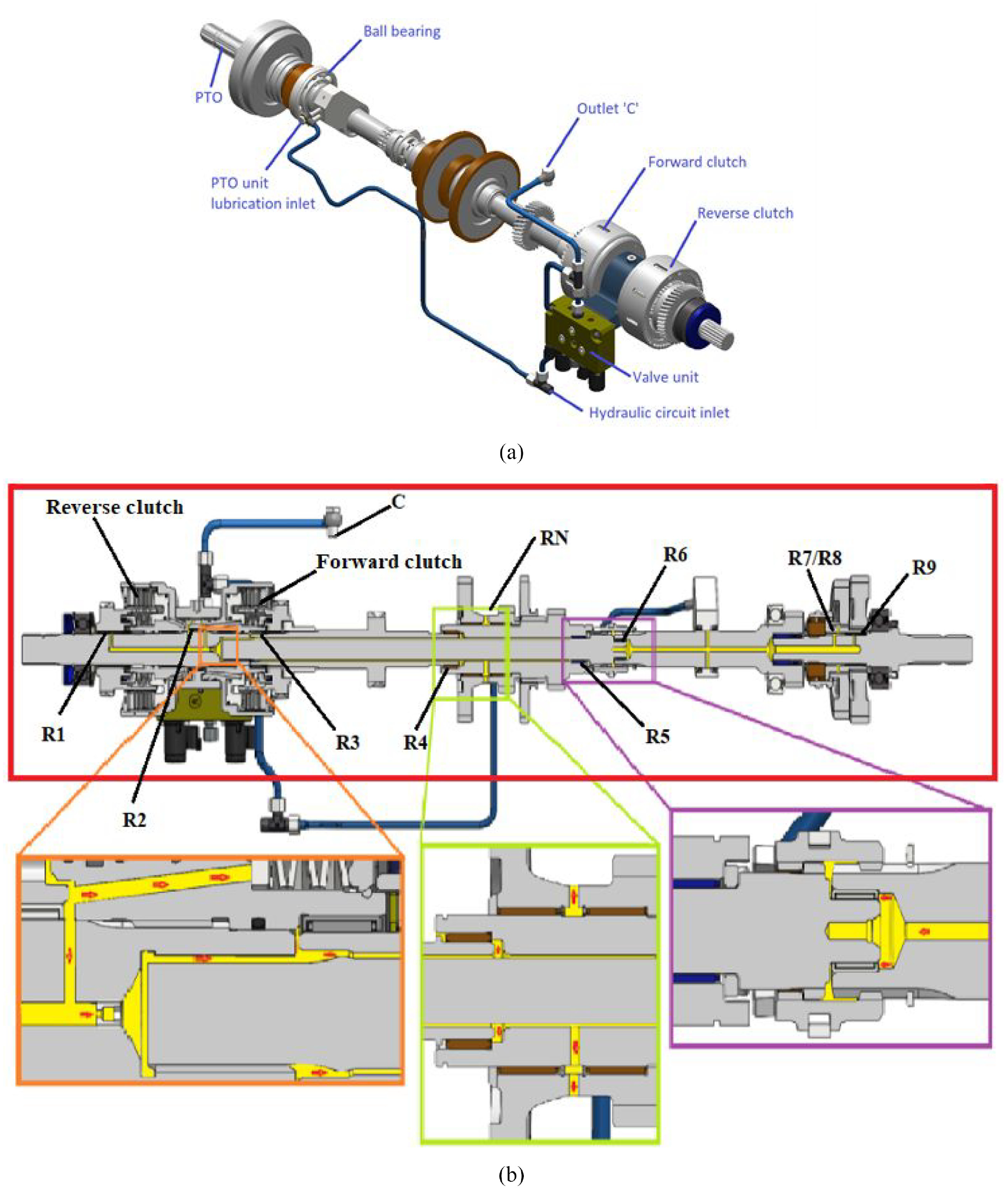
(a) Isometric view of transmission part under study and (b) section view of transmission part under study.

Computational models

Methodology used

The goal of the analysis methodology is to obtain a reliable and efficient software model of the LUB circuit. To achieve these purposes, an analysis of the hydraulic circuit was first made, which consisted of two circuits in series, one at higher pressure in order to operating the clutches and one for LUB.

The entire circuit was then modeled with LP with the use of a commercial LP code, from the results obtained it was possible to establish the amount of flow directed to the power transmission control circuit and those to the LUB circuit. The LUB flow rate from the LP model is used as input for the CFD model, which determines the flow rate values at each outlet.

The flow rate values at the outputs calculated with LP modeling were compared with those calculated by CFD analysis, for unacceptable deviation values between the corresponding output flow values between the two models, a calibration of the LP model was carried out through an iterative process, so that it reproduces as much as possible the behavior determined by the CFD model.

The reason for these choices is to be found in the intrinsic characteristics of the two models, the modeling of the entire circuit with LP made it possible to derive the value of the LUB flow keeping low the computational effort and with a good level of approximation.

The value of the inlet flow rate $Q_{lubeInlet}$ to the LUB circuit is obtained by subtracting from the known total flow rate of the system ( $Q_{tot}$ ) the flow rate of the power transmission control circuit ( $Q_{A . P . Inlet}$ ) for the actuation of clutches, id est:

Q_{lubeInlet} = Q_{tot} - Q_{A . P . Inlet}

(1)

The power transmission control part of the circuit is composed of manifolds of shapes that can be appropriately reproduced through the union of components available in the 1D commercial code’s libraries. The long and established practice of simulation of hydraulic controls can reassure that the result obtained agrees with the real condition.

The previous considerations do not apply to the LUB circuit, due to the complexity of the geometry, for which the use of a 3D model is necessary.

The comparison between the results of the two models and the calibration of the LP model brings a fast and effective model that can be used to optimize the circuit, in fact, it accurately reproduces the behavior of the LUB circuit and makes it possible to test numerous combinations with a reduced computational effort, with much shorter timelines than a CFD analysis or experimental tests that would be inadequate to respect the classic industrial timings.

This methodology is summarized by Figure 3 where Circuit 1D A.P. is the LP model of the power transmission control circuit, Circuit 1D lube is the LP model of the LUB circuit and together these two models constitute the LP model of the entire hydraulic circuit, $Q_{lube 1 D}$ are the flows to the outlets determined with the LP model, $Q_{lube 3 D}$ are the flows to the outlets determined with the CFD model.

Figure 3.

Analysis methodology.

Lumped parameter model of the hydraulic circuit

The circuit consists of four main branches. Two are for the control of the clutches, respectively, of Forward and Reverse. Two are for LUB of the front components and components of the PTO, respectively. The color of the submodels identifies the library. Pink submodels belong to the hydraulic resistance library²¹ modeling of pressure drops versus flow rates in hydraulic networks that takes the coefficients from an internal library based on well-founded engineering databases such as Idel’cik.²² Blue submodels belong to the hydraulic library dedicated to the design of general hydraulic systems. The red submodels belong to the signal and control library which makes it possible to construct logic block diagram models. Green submodels belong to the 1D mechanical library. Each branch consists of different library submodels. The clutches control branch also include mechanical submodels representing the actuators moving masses and springs. The circuits for the control of frictions consist of 8 general hydraulic, 25 hydraulic resistance, 1 signal, and 3 mechanical submodels. The circuit for the LUB of the front components consists of 19 general hydraulic, 80 hydraulic resistance, and 11 signal submodels. The PTO LUB circuit consists of 9 general hydraulic, 56 hydraulic resistance, and 3 signal submodels. In the LP model the submodels are described using nonlinear time-dependent analytical equations that represent the behavior of the system.

In order to determine the flow rate and pressure drop throughout the LUB circuit, the first step consists in applying mass conservation principles at each junction within the LUB system. Assuming that the CFD results have shown—as confirmed in the next sections—the absence of major effect of cavitation, the continuity equation in a node for incompressible flow is:

\sum_{i = 1}^{n} Q_{i} = 0

(2)

where “ $Q_{i}$ ” is the volumetric flow rate at the node of the i-th branch.

Next, the conservation of energy per unit of mass along the same streamline can be enforced. In the case of incompressible flow along the streamline, the energy balance equation can be expressed as follows:

\frac{p_{a}}{γ} + \frac{v_{a}^{2}}{2 g} + z_{a} = \frac{p_{b}}{γ} + \frac{v_{b}^{2}}{2 g} + z_{b} + h_{f}

(3)

where, $p_{a}$ , $p_{b}$ , and $v_{a}$ , $v_{b}$ , and $z_{a}$ , $z_{b}$ are, respectively, the pressure, velocity, and elevation at the points located in a and b, $h_{f}$ represent the frictional pressure drop, $γ$ is the specific gravity of the fluid, $g$ is the gravity acceleration.

The pressure drop along a pipe for incompressible flow is determined by the Fanning equation, which is derived from the energy equation.

p_{a} - p_{b} - ρ f (Q, D) \frac{8 Q^{2}}{D^{4}} (\frac{L}{D} + \frac{K}{f (Q, D)}) - γ (z_{b} - z_{a}) = 0

(4)

where, $K$ is the dimensionless coefficient obtained experimentally taking into account the load losses in the curves, elbows, T joints, etc.²³

$ρ$ is the density of the fluid, $Q$ the volumetric flow rate, $D$ and $L$ are, respectively, the diameter and length of the pipe. $f$ is a friction factor for pipes with a circular cross section.

The friction factor for turbulent flow can be decided from the Reynolds number ( $R_{e}$ ), the velocity ( $v$ ), and the Hazen-William constant ( $C$ ). Here, for convenience, the transient region is included in the turbulent region. For the smooth tube, $C$ is 140.

For laminar flow, $R_{e} \leq 2000$

f (Q, D) = \frac{64}{R_{e}}

(5)

For turbulent flow, $R_{e} > 2000$

f (Q, D) = 1304.56 \frac{v^{0, 0184}}{C^{1, 852} {R_{e}}^{0, 1664}}

(6)

where $R_{e}$ , can be expressed as $4 ρ Q / π μ D$ , μ is the dynamic viscosity of the lubricant.

Pipe friction is taken into account using a friction factor based on the Reynolds number $R_{e}$ , and relative roughness. For ease of reference, the transitional region is here considered as part of the turbulent region.²⁴

The general expression of centrifugal pressure $p_{c}$ is:

Δ p_{c} = \frac{1}{2} ρ ω^{2} R^{2}

(7)

where, $ρ$ is the density of the fluid, $ω$ represents the angular velocity of the shaft, $R$ is the radial distance from the axis of rotation.²⁵

The inclusion of Coriolis forces would be necessary for completeness; however, it was verified by Marani et al.¹⁷ that their influence is quite insignificant for this environment.

Domain geometry

The LUB circuit consists of various fluid passages and volumes inside the transmission assembly. Simulating these volumes is challenging because of the complexity and accuracy of the solid model.

In the LP model, the real geometry was recreated by coupling elements with the most possible similar shapes to those of the LUB circuit components. The result of this process is shown in Figure 4.

Figure 4.

Lumped-parameter model.

CFD model

The 3D CAD geometry is created in the solid modeler, this is then imported into the meshing, after that a tetrahedral mesh and a hybrid grid tetrahedral mesh with prismatic layers were generated by means of ANSYS ICEM CFD 2021 R1.²⁶ The virtual simulations were performed with the commercial CFD code ANSYS CFX 2021 R1.²⁷ The software utilizes a finite element-based finite-volume method to solve the 3D Reynolds-averaged form of the Navier-Stokes equations. To compute the advection terms in the discrete finite-volume equations, a second-order high-resolution advection scheme was employed.

The Navier-Stokes equations are a system of three balance equations (partial differential equations) of continuum mechanics, which describe a linear viscous fluid; in them Stokes’ law (in the kinematic balance) and Fourier’s law (in the energy balance) are introduced as constitutive laws of the material.

The Navier-Stokes equation (8) is composed of three scalar equations that must be used together with the Continuity equation (9).²⁸

ρ \frac{D \bar{v}}{Dt} = - \nabla p - ρ \nabla Ψ + \nabla \cdot \bar{\bar{τ}}

(8)

\frac{\partial ρ}{\partial t} + \nabla \cdot (ρ \bar{v}) = 0

(9)

where $\bar{\bar{τ}}$ is the deviator stress components and $\nabla Ψ$ represents body accelerations acting on the continuum $(Ψ = gz)$ .

The introduction of the Reynolds mean generates further unknowns, because the division of the variables into an average component plus a fluctuating one generates a further term within the stress tensor: the Reynolds stresses. To close the problem, the hypothesis introduced by Boussinesq is used. For the solution of the problem, the code must calculate six variables in six partial differential equations, which are: the continuity equation, the momentum equation of the quantity of motion (which being vector is broken down into three equations), and the equations for turbulence.

The target of the simulation is the assessment of the flow rates at the lubricating members, therefore, with the help of the function calculator tool offered by the code in the post-process phase, the mass flow rate was calculated for each surface. The pressure drop is calculated by the difference of the total pressure calculated in the outlet and inlet sections, $p_{02}$ and $p_{01}$ , respectively.

Δ p_{0} = p_{02} - p_{01}

(10)

where $p_{0}$ is the static pressure averaged over the local mass flow that can be obtained by the general expression reported in equation (11) where $ϕ$ represents any variable or expression being averaged ( $p_{0}$ in this case) and $m$ represents the local mass flow:

ϕ = \frac{\sum (m ϕ)}{\sum m}

(11)

To get to the results, the calculation times are in the order of few minutes for the LP model and 1.5 days for the CFD model using a computer with Intel Xeon processor CPU E5-1620 3.60 GHz and 16 Gb of RAM. The number of iterations needed to reach convergence is at least 500.

Fluid domain

For the CFD model the domain was obtained starting from the 3D CAD drawing and keeping only the surfaces wetted by the lubricant. The domain obtained, occupied by the fluid, is represented in the Figure 5.

Figure 5.

Fluid domain.

Numerical grid

Several grids were created, generated by 3D commercial code, the first mesh created was uniform and made up of tetrahedral elements.

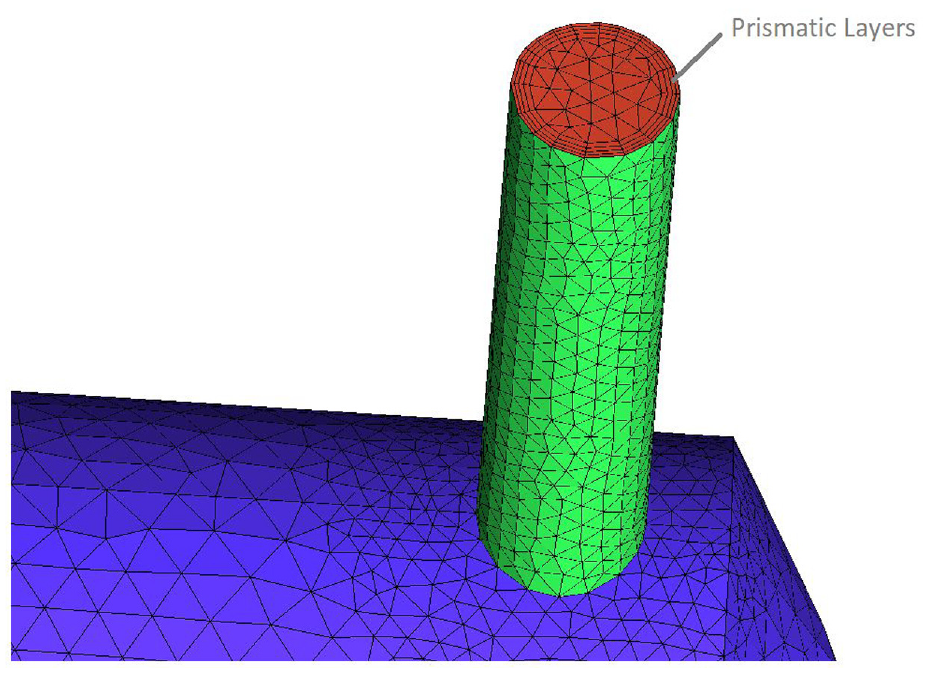
The use of tetrahedral cells can save a significant amount of time as the process of grid generation is automated. Additionally, due to the complex geometries of LUB circuits, generating hexahedral cells can be a time-consuming process, which may not be feasible to meet industrial scheduling requirements. The initial two meshes were inadequate in describing the behavior of the flow due to their low number of elements. This insufficiency was particularly noticeable in the thinner sections and outlets. To overcome this issue, a third mesh was created with a lower maximum element size and constraints placed on elements belonging to restricted areas or neighboring surfaces, resulting in a finer tetrahedral mesh with local refinements in gaps. Later on, a tetrahedral and prismatic hybrid mesh was selected, with four prismatic wall layers added to accurately solve the boundary layer. By setting the height of the first prism layer to 0.02 mm, a value of $y + < 2$ was achieved on all surfaces. The mesh quality was checked by analyzing the properties of the elements, such as the Orthogonality Angle, the Expansion Factor, and the Aspect Ratio. The orthogonality angle and aspect ratio are criteria used to measure the distortion of the elements, while the expansion factor measured the uniformity of the mesh. In Table 1 the values of these properties are reported for each generated mesh.

Table 1.

Properties of the elements.

Mesh	Orthogonality angle (°)	Expansion factor (-)	Aspect ratio (-)
Mesh 4	0.72	1.00	0.69
Mesh 3	0.81	1.00	0.79
Mesh 2	0.79	1.00	0.77
Mesh 1	0.71	1.00	4.16

The best compromise between the quality of the grid (distortion of the elements) and the number of elements was found when in the narrowest spaces a minimum of eight prismatic layers and four tetrahedral elements are generated and that at the outputs a minimum of eight prismatic layers and six are generated tetrahedral elements on the diameter. Details of this mesh are shown in Figures 6 and 7.

Figure 6.

Partial detail of the hybrid mesh section.

Figure 7.

Detail of hybrid mesh.

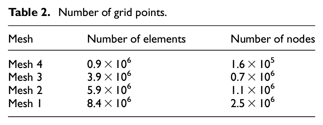
Four different meshes with a different number of grid points (Table 2) were generated and tested to evaluate the sensitivity to the grid.

Table 2.

Number of grid points.

Mesh	Number of elements	Number of nodes
Mesh 4	0.9 × 10⁶	1.6 × 10⁵
Mesh 3	3.9 × 10⁶	0.7 × 10⁶
Mesh 2	5.9 × 10⁶	1.1 × 10⁶
Mesh 1	8.4 × 10⁶	2.5 × 10⁶

The parameters used to evaluate this aspect were the pressure at the inlet and at R6 and R9 outlets in relation to the number of elements of the mesh used for their determination.

The test showed that a minimum number of at least 5.9 × 10⁶ elements should be used to ensure grid independence. The final mesh includes 8.4 × 10⁶ elements and was obtained with four prismatic layers added on all surfaces of the fluid domain to correctly resolve the boundary layer. The increase in the number of elements was carried out considering the size of channels of the domain, in the chosen mesh there are at least eight prismatic layers and four tetrahedral elements in the narrow channels.

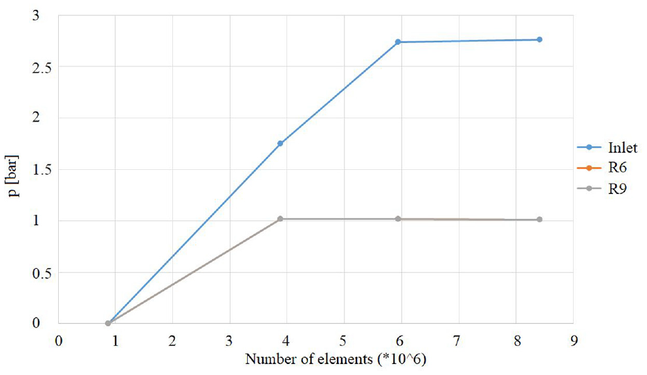
The inlet pressure ( $p_{inlet}$ ), Figure 8 shows that with a number of elements at least equal to that of the densest tetrahedral mesh, the results do not change significantly as the number of nodes increases, with Mesh 4 $p_{inlet} = 0 bar$ , with Mesh 3 $p_{inlet} = 1.75 bar$ , with Mesh 2 $p_{inlet} = 2.74 bar$ , with Mesh 1 $p_{inlet} = 2.76 bar$ , so the grid independent condition has been reached.

Figure 8.

Grid independent analysis.

Figure 8 displays the pressure variation at R6 and R9 outlets for increasing number of mesh elements. The graph indicates that the pressure at R6 outlet remains constant when the number of nodes is at least equal to that of Mesh 3. Specifically, Mesh 4 resulted in a pressure of 0 bar, Mesh 3 produced a pressure of 1.02 bar, Mesh 2 produced a pressure of 1.02 bar, and Mesh 1 produced a pressure of 1.01 bar. Therefore, the grid-independent condition has been achieved. Similarly, the pressure at the R9 outlet was found to be constant for Mesh 3 and above, with Mesh 4 yielding a pressure of 0 bar, Mesh 3 producing a pressure of 1.02 bar, Mesh 2 producing a pressure of 1.02 bar, and Mesh 1 producing a pressure of 1.01 bar. This indicates that Mesh 2 or Mesh 1 produced more reliable results, as the number of nodes did not significantly impact the outcome.

In conclusion, Mesh 1 was chosen due to its satisfactory level of result accuracy with reasonable computational effort.

Boundary conditions

The simulations were performed in stationary conditions. The Dirichlet boundary condition of static pressure ( $p_{s}$ ) has been imposed on all outlets, $p_{s} = p_{atm}$ ∀ outlet, as they are all connected to $p_{atm}$ both directly and through components such as bearings that have flow passage areas greater than several orders of magnitude with respect to the size of the LUB ducts which precede them. For the CFD model, the mass flow rate was set in accordance with the data obtained from the LP model for the LUB part of the circuit, $Q_{CFD} = Q_{lubeInlet}$ . Boundary conditions, such as those imposed, of mass flow inlet and pressure at outlet are robust conditions. The simulations were isothermal, the pressure variations within the circuit are not such as to make relevant for this study the variations of density and viscosity that they would entail, so the fluid maintains a constant temperature, density, and viscosity. The properties of the fluid, which is a Universal Tractor Transmission Oil and is classified as SAE grade 10W-30, were taken into account for the typical operating conditions of the transmission regime, they are shown in Table 3. Being a standard mineral oil, it is Newtonian, this data was accordingly used in the models.

Table 3.

Characteristics of the lubricating fluid.

Density	850 kg/m³
Kinematic viscosity	60 cSt
Dynamic viscosity	51 cP
Temperature	80°C

A Menter Baseline Turbulence model (BSL k-ω) has been enforced instead of a k-ε because it is more suitable for near-wall flow regions and accurately captures the fluid flow behavior in the boundary layer. It is good at resolving internal flows, separated flows, and flows with high-pressure gradients, as well as internal flows through curved geometries. The $R_{e}$ has been calculated in different areas of the fluid domain, since its value exceeds 400 in numerous areas of the fluid domain. These factors make the BSL k-ω robust and versatile choice for turbulence modeling in this application. The calibration constants for this model are $σ_{k 1} = 2$ and $σ_{ω 1} = 2$ near the wall and $σ_{k 2} = 1$ and $σ_{ω 2} = 1 / 0.856$ in the domain and represent the coefficients of the $ω$ -eq12. The developed CFD model uses a coupled solver, which solves the hydrodynamic equations as a single system. This solution approach uses a fully implicit discretization of the equations.

Numerical uncertainty

The convergence criterion selected compatibly with the type of problem was to achieve residual values relating to the equations of the momentum and conservation of mass at least in the range of 10⁻⁴/10⁻⁵.

To assess the discretization error, the GCI method was employed. This method relies on the Richardson extrapolation technique and has been extensively evaluated across a wide range of CFD cases, making it a reliable and recommended approach.²⁹ The calculation of the fine-GCI ( ${GCI}_{fine}^{21}$ ) passes through the calculation of the representative mesh size ( $h$ ), of the apparent order ( $p_{a . o .}$ ), of the approximate relative error ( $e_{a}^{21}$ ) and of the extrapolated relative error ( $e_{ext}^{21}$ ).

The GCI_fine²¹ is calculated as:

{GCI}_{fine}^{21} = \frac{1.25 e_{a}^{21}}{r_{21}^{p_{a . o .}} - 1}

(12)

The apparent order (p_a.o.), is calculated as:

p_{a . o .} = \frac{1}{\ln (r_{21})} | \ln | ε_{32} / ε_{21} | + \ln (\frac{r_{21}^{p_{a . o .}} - s}{r_{32}^{p_{a . o .}} - s}) |

(13)

where $s = 1 * sing (\frac{ε_{32}}{ε_{21}})$ , $ε_{32} = ϕ_{3} - ϕ_{2}$ , $ε_{21} = ϕ_{2} - ϕ_{1}$ .

The approximate relative error (e_a²¹) is calculated as:

e_{a}^{21} = | \frac{ϕ_{1} - ϕ_{2}}{ϕ_{1}} |

(14)

The extrapolated relative error (e_ext²¹).

e_{ext}^{21} = | \frac{ϕ_{ext}^{21} - ϕ_{1}}{ϕ_{ext}^{21}} |

(15)

Table 4 shows the data relating to the case under study, where $N_{k}$ with $k = 1, \dots, 3$ is the number of elements of the generated mesh, $ϕ_{k}$ the critical variable (in this case the inlet pressure), $ϕ_{ext}^{21}$ and $ϕ_{ext}^{32}$ the extrapolated values, calculated as:

ϕ_{ext}^{21} = (r_{21}^{p_{a . o .}} ϕ_{1} - ϕ_{2}) / (r_{21}^{p_{a . o .}} - 1)

(16)

Table 4.

Calculation of discretization error.

Discretization error
$N_{1}$	8410000
$N_{2}$	5940000
$N_{3}$	3880000
$r_{21}$	1.142
$r_{32}$	1.157
$ϕ_{1}$	2.76
$ϕ_{2}$	2.74
$ϕ_{3}$	1.75
$p_{a . o .}$	26.698
$ϕ_{ext}^{21}$	2.761
$ϕ_{ext}^{32}$	2.761
$e_{a}^{21}$	0.725%
$e_{ext}^{21}$	0.0217%
${GCI}_{fine}^{21}$	0.0268%

And similarly for $ϕ_{ext}^{32}$ .

In addition, $r_{21}$ e $r_{32}$ are the grid refinement factors between Mesh 2 and 1 and between Mesh 3 and 2 calculated as:

r = h_{coarse} / h_{fine}

(17)

where $h$ is calculated as

h = {[\frac{1}{N} \sum_{i = 1}^{N} Δ V_{i}]}^{1 / 3}

(18)

where $V_{i}$ is the volume of the ith cell. $r_{21}$ e $r_{32}$ should be greater than 1.3. According to Celik et al.²⁹ it was not possible to comply with this indication due to the already high number of elements of the mesh, but since this is a recommended heuristic value rather than a formal derivation, the convergence was considered granted, basing on relative and extrapolated error. In fact, the approximate relative error between the two best meshes results 0.725% and of the extrapolated relative error result of the best mesh equals 0.0217%. The iteration error on the variable calculated with the method described by Celik et al.²⁹ is not reported because it is considered negligible, therefore the simulation is considered to be convergent.

Results

The LP model was run in parallel obtaining the results shown in Figure 9 prior to the calibration process. Instead, Figure 10 shows the results of the CFD model, note that all the results are normalized to 100 for non-disclosure reasons. I1 and I3, the outputs of the clutch actuation valves are included only in the LP results being part of the power transmission control circuit. By comparing with the CFD results, a large flow discrepancy is outlined across different outlets; for example, flow to outlet R1 goes from 7.80% of the input flow rate with LP model to 4.05% with CFD model, flow to outlet R6 goes from 10.04% with LP model to 6.05% with CFD model, flow to outlet R7/R8 goes from 0.15% with LP model to 2.11% with CFD model. One important result is that the CFD modeling shows that the pressure head created by the centrifugal force don’t give rise to negative relative pressure which is confirmed by outgoing flows from all the outlets. Therefore, the phenomena of air intake from the external space studied in Ferrari and Marani³⁰ do not occur. Being circuits with marked dimensional differences, even of orders of magnitude, cavitation can occur but localized only in particular points due to the fluid local acceleration but the phenomenon expires as soon as the fluid decelerates to the steady velocity. In particular, it could occur after bottlenecks, downstream of the clutches on the central shaft where the pressure is lower (Figure 9). These considerations lead us to affirm that, being a globally single-phase flow, a LP model can be used for its study. We authors, in previous works, have shown that, if the flow is two-phase, the LP environment (based on single phase fluid physics equations) hasn’t the capability of catching the phenomena and in these cases the modeling should be done with CFD tools. The differences between LP and CFD results have made necessary to calibrate the LP model on the basis of the CFD model particularly in three points of the circuit and were consistent and reasonable with respect to the simplifications introduced and consequently with the deviations deriving from them. The first difference concerned the LUB distributor which did not introduce a sufficient pressure drop, its equivalent diameter has been changed from 21.16 to 8 mm.

Figure 9.

LP model results in reverse, in stationary before calibration.

Figure 10.

CFD model results in reverse, in stationary.

The second variation concerned R6 output, where it was necessary to insert an equivalent choke of 3.4 mm diameter to represent the pressure drops given by the passage through the roller bearing seats.

The third modification concerned C outlet dedicated to bearing LUB, the choke of 1 mm diameter that represented the outlet nozzle was replaced by a restriction and a duct with a diameter of 1 mm and length of 5 mm equal to those of the nozzle.

The intermediate results of iterative process used for calibration of LP model are shown in Figure 11.

Figure 11.

Intermediate results of iterative process used for calibration of LP model.

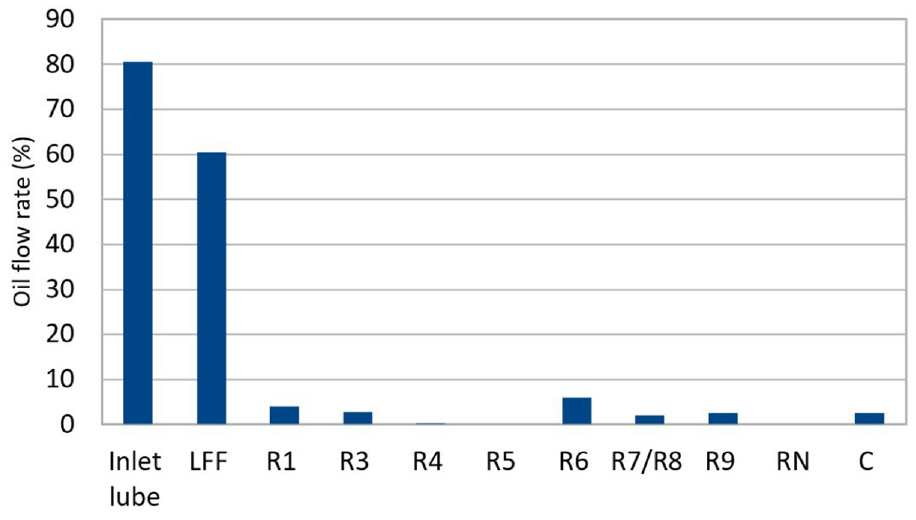
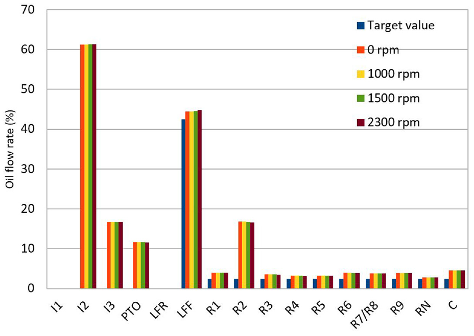
The results obtained in this way show a good consistency: the flow rates are all outgoing, the sum of the outlets corresponds to the inlet flow rate, the Figures 12 and 13 show the inlet and outlet flow rates as a percentage of the volumetric flow rate entering the transmission.

Figure 12.

Oil flow values in reverse.

Figure 13.

Oil flow values in forward.

Figures 12 and 13 show the flow rate values expressed as a percentage of the overall transmission capacity obtained, respectively, in the conditions with the clutch engaged as reverse and forward with the calibrated model developed in the 1D commercial code.

The results differences between the model developed in the 1D commercial code after the calibration and the model developed in the 3D commercial code are negligible and the LP model thus obtained offers a reduced computational effort and can be used to optimize the distribution of the flow rates to the various outlets by testing multiple combinations in short time. With the LP model obtained it is possible to numerically vary the diameters of the calibrated orifices in the circuit, until the optimal LUB flow rate is reached at the outlets with a fast and effective method, while a CFD approach would go through the time consuming steps of changing the 3D model, Meshing, Solving, and Post Processing.

Looking at the results, we can highlight the most critical parts of the LUB circuit. The flow rate at the R6 output is almost double that of the target, resulting in a reduction in the energy efficiency of the transmission. On the contrary, the flow rates at the RN, R5, and R4 outlets are much lower than the desired ones.

Figure 14 shows a contour plot of the pressure, it is observed a high pressure gradient in the section changes, and friction losses distributed along the external pipes.

Figure 14.

Contour plot of the pressure of the lubrication circuit.

The most important local friction losses are in the inlet, in the section changes, and in the crossing of the meatus of the groove ad hoc created by the removal of a tooth.

RN and R5 bearings are characterized by the lowest lubricant flow rates and the furthest from the LUB target, since they are those located at the greatest distance from the LUB inlet into the shaft and where the pressure is very low.

Vice versa, the flow rate to the roller bearing R6 is much higher than the target value.

Figure 15 represents a velocity streamline. The streamlines represent the flow path of the particles, in this case a rectilinear trajectory is shown: the axial movement is a consequence of the pressure differentials. The flow rate of the central channel is decreasing from the inlet to the furthest outlets and due to the flow coming out from the radial ducts, the axial velocity component drops.

Figure 15.

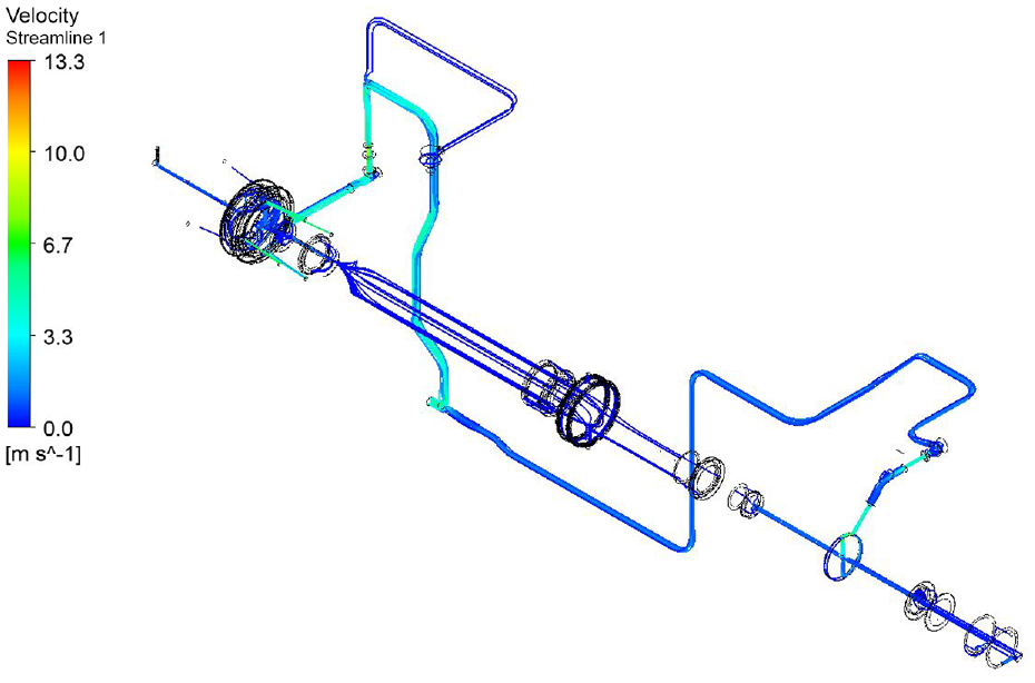
Velocity streamline of the flow of the lubrication circuit.

The LP model gives the opportunity to easily optimize the circuit and to correct the problems discussed above particularly on insufficiently lubricated outlets. To obtain this result, the diameters of the outlets and screw precision orifices were varied and the appropriate calibrated orifice was inserted obtaining the results shown in Figures 16 and 17.

Figure 16.

Oil flow values in reverse after circuit optimization.

Figure 17.

Oil flow values in forward after circuit optimization.

In the end, the flow rate, expressed as a percentage of the overall transmission capacity and obtained with the reverse and forward clutch engaged, respectively, meet the targets in each condition, thanks to the newly calibrated LP model, developed after a fast optimization process of the LUB circuit.

Conclusion and future perspectives

The design of the LUB circuits is based on good practice design rules and on “trial and error.” Experimentally, the LUB can only be verified with the simplified condition of stationary transmission. The rotation of the transmission shafts generates centrifugal forces in the oil which moves in the circuit. Testing the stationary transmission means completely neglecting the centrifugal effect which has a fundamental importance in the distribution of the oil inside the circuit. The analysis methodology presented here can lead to a sort of virtual testing of the circuit and can be used to verify the correct design of a LUB circuit and allows to optimize flows by making rapid geometric changes.

In this work, the problem described above is tackled by analyzing the LUB circuit of an agricultural transmission using an LP and a CFD approach, finally obtaining a hybrid LP model to produce accurate results with low computational effort, defining a new analysis methodology. The model obtained was used to optimize a real isometric 75 kW tractor LUB circuit.

The results showed that the hybrid LP model offers a good prediction of the circuit while keeping the computational effort low. The problems encountered with the LP model regard the modeling of complex geometries because it models equivalent choke area and is not affected by three-dimensional effects.

The drawbacks encountered with the CFD model are the high computational effort and long times required to obtain the geometry of the domain, to create the mesh, to run the model, to obtain the grid independence, and to do the uncertainty analysis.

The methodology adopted in this study shows how it is possible to combine the advantages of both approaches of modeling. The resulting hybrid model is faster than a CFD-only model and more accurate than an LP-simple model. No existing studies develop an LP model calibrated with a CFD model to optimize the internal LUB of a mechanical transmission. Furthermore, the literature CFD studies on this topic are rare and mostly focused on external LUB.

In the view of the fact that experimental validation cannot be practically obtained, the validity of the presented model is confirmed by previous experiences^16,17,29 and the results are consistent with industrial know-how.

With the developed model, critical issues were highlighted in the LUB circuit designed according to good design rules and prediction errors in the LP model. The developed model allowed to overcome both problems and to optimize the LUB circuit, achieving a better balance of oil flows among the various outlets and reaching the target values.

The presented method has impacted positively in the process of design of the transmission of a new tractor, which is a field where, still nowadays, no well-established methods are available for the design of LUB circuits.

The simulations were performed under isothermal conditions because it is a very good approximation of the steady-state operating condition, but the developed model can also be used for different temperatures or with lubricants of different characteristics.

The relatively simple architecture and the operating conditions of this transmission has allowed to use an approximate model without requiring to take into account of the effects of oil splashing which could possibly reduce the flow rate in the circuit. Moreover as the supply flow rate gets lower and rotational speed increase the air ingestion in the system becomes more and more likely. Thus to consider these effects, a much more complex, dynamic and two-phase model would be needed.³⁰ A furthermost advancement would be the integration of Multiphase CFD models able to assess the LUB performance in conditions close to the saturation pressure, until the arise of two phase flow.

Footnotes

Appendix

Acknowledgements

We would like to express our sincere gratitude to the technical director Ing. Marcello Conatrali of BCS-Ferrari in Luzzara (RE), Italy, for his valuable support throughout this research project. His availability was crucial for the successful completion of this work.

Handling Editor: Sharmili Pandian

Author contributions

Conceptualization, Giorgio Paolo Massarotti; Methodology, Cristian Ferrari; Software, Luca Magri; Validation, Pietro Marani; Investigation, Luca Magri; Resources, Giorgio Paolo Massarotti; Writing—original draft, Luca Magri; Writing—review & editing, Pietro Marani; Supervision, Cristian Ferrari.

Declaration of conflicting interests

The author(s) declared no potential conflicts of interest with respect to the research, authorship, and/or publication of this article.

Funding

The author(s) received no financial support for the research, authorship, and/or publication of this article.

ORCID iD

Cristian Ferrari

References

RS.

Digital simulation of engine lubrication systems. SAE Paper 710205, 1971.

Neu

Wade

Chu

AC.

Simulating the lubrication system of a diesel engine. SAE Paper 770032, 1977.

Chun

Park

Y H

Jang

A study on engine lubrication system by optimized network analysis—part I: case study. SAE 2000-01- 2921, 2000.

Chun

Park

Jang

A study on engine lubrication system by optimized network analysis—part II: parametric study. SAE 2000-01- 2923, 2000.

Ning

Meixiang

Hongying

, et al. Simulation of automotive engine lubrication system based on AMESim. Appl Mech Mater 2012; 235: 239–244.

Felix

Uwe

Simulating engine lubrication systems with 1-D fluid flow models. In: SAE world congress in Detroit, Michigan, 2000.

Ryu

Kim

KU.

Power efficiency characteristics of a tractor drive train. Trans ASAE 2003; 46: 1481–1486

Renius

Resch

Continuously variable tractor transmissions. Trans ASAE 2005; 29: 1–37.

Schembri Volpe

Carbone

Napolitano

, et al, Design optimization of input and output coupled power split infinitely variable transmissions. J Mech Des 2009; 131: 111002.

10.

Pahlovy

Mahmud

Kubota

, et al. Multiphase drag modeling for prediction of the drag torque characteristics in disengaged wet clutches. SAE International 2014-01-2333, 2014.

11.

Hohn

Michaelis

Otto

. Influence on no-load gear losses. In: Proceedings of the ecotrib conference, 2011, vol. 2, pp. 639–644. https://www.researchgate.net/publication/304822767_Influences_on_noload_gear_losses?_tp=eyJjb250ZXh0Ijp7ImZpcnN0UGFnZSI6Il9kaXJlY3QiLCJwYWdlIjoiX2RpcmVjdCJ9fQ

12.

Yuan

Attibele

Dong

. CFD simulation of the flows within disengaged wet clutches of an automatic transmission. SAE International 2003-01-0320, 2003.

13.

Takagi

Nakata

Okano

, et al. Effect of two-phase flow on drag torque in a wet clutch. J Adv Res Phys 2011; 2: 021108.

14.

Concli

Gorla

. Computational and experimental analysis of the churning power losses in an industrial planetary speed reducers. In: Ninth international conference on advances in fluid mechanics—advances in fluid mechanics IX, WIT transactions on engineering sciences. WIT Press, 2012, vol. 74, pp. 287–298. DOI: 10.2495/AFM120261.

15.

Concli

Gorla

. Oil squeezing power losses of a gear pair: a CFD analysis. In: Ninth international conference on advances in fluid mechanics—advances in fluid mechanics IX, WIT transactions on engineering sciences. WIT Press, 2012, vol. 74, pp. 37–48. DOI: 10.2495/AFM120041.

16.

Gorla

Concli

Stahl

, et al. CFD simulations of splash losses of a gearbox. Advances in Tribology 2012; 616923.

17.

Marani

Ferrari

Paoluzzi

, et al. Methods of computational fluid dynamics for a CVT transmission lubrication system of agricultural tractor. In: Proceedings of the 9th international fluid power conference, Aachen, 24–26 March 2014, vol. 3, pp. 555–565, 9th IFK.

18.

Ferrari

Marani

Ghorpade

. CFD modeling of lubrication system in agricultural power split transmission. In: Proceedings of the 13th european conference of the international society for terrain vehicle systems, Roma, 21–23 October 2015, pp. 627–639.

19.

Jiang

, et al. Optimized design of the flow networkin the lubrication system for the heavyvehicle transmission. Adv Mech Eng 2017; 9: 1–16.

20.

Mastrone

Concli

CFD simulations of gearboxes: implementation of a mesh clustering algorithm for efficient simulations of complex system’s architectures. Int J Mech Mater Eng 2021; 16: 12.

21.

Simcenter Amesim. 2019.2. Simcenter Amesim help. Munich: Siemens Aktiengesellschaft, 2019.

22.

Idel’cik

IE.

Handbook of hydraulic resistance. 4th ed revised and augmented. Moscow, Russia: Research Institute for Gas Purification, 2008.

23.

Streeter

Wylie

. Fluid mechanics. New York: McGraw-Hill, Inc, 1979. https://archive.org/details/fluidmechanic00stre.

24.

White

FM.

Fluid mechanics. New York: McGraw-Hill Inc., 1986. https://archive.org/details/fluidmechanics0000whit.

25.

Chun

SM.

Network analysis of an engine lubrication system. Tribology Int 2003; 36: 609–617.

26.

Ansys Inc. Ansys ICEM CFD user manual. Canonsburg, PA: Ansys Inc., 2021b.

27.

Ansys Inc. CFX solver theory guide R1. Canonsburg, PA: Ansys Inc., 2021a.

28.

Johnson

RW.

The handbook of fluid dynamics. Boca Raton, Fla.: CRC Press, 1998. https://archive.org/details/handbookoffluidd0000unse_b1m7.

29.

Celik

Ghia

Roache

, et al. Procedure for estimation and reporting of uncertainty due to discretization in CFD applications. ASME J Fluids Eng 2008; 130(7): 078001. DOI: 10.1115/1.2960953.

30.

Ferrari

Marani

. Study of air inclusion in lubrication system of CVT gearbox transmission with biphasic CFD simulation. In: Proceedings of the Bath/ASME symposium on fluid power and motion control, FPMC2016, 7–9 September 2016, Bath, UK.

A methodology for predicting and optimizing the lubrication of an off-road machine transmission

Abstract

Keywords

Introduction

Geometry of the transmission

Computational models

Methodology used

Lumped parameter model of the hydraulic circuit

Domain geometry

CFD model

Fluid domain

Numerical grid

Boundary conditions

Numerical uncertainty

Results

Conclusion and future perspectives

Footnotes

Appendix

Acknowledgements

Author contributions

Declaration of conflicting interests

Funding

ORCID iD

References