Sage Journals: Discover world-class research

Abstract

This paper suggests that the long-range dependence (LRD) in acoustic signal is an important indicator of dynamic behavior in data. Considering this information, a novel framework based on LRD in acoustic is proposed for detecting change-points in machine running status. Initially, the LRD phenomenon in acoustic is demonstrated. Subsequently, a change-point detection framework is developed, leveraging LRD to monitor machine running states. The framework includes two phases: (1) characteristic data prediction: the LRD value is predicted by the fractional autoregressive integrated moving average (FARIMA) model, which is applied to reflect changes in machine operation states. (2) date change detection: based on residual analysis, a null hypothesis testing based automatic analysis method for acoustic signals during machine successive operations is used to make decision. Experiments in real-world applications demonstrated the good potential of the proposed framework in practical engineering scenarios.

Keywords

Change detection acoustical signal long-range dependence factional autoregressive integrated moving average

Introduction

Real-world industrial machines rarely operate stably, but are almost always unstable with temporal variations.¹ Consequently, modern industries are increasingly seeking methods to automatically monitor the dynamic running statuses of these machines, and to identify their potential status changes caused by abnormalities, faults, and switching points at an early. Here, the problem of change point detection (CPD) is regarded as when a structural change in the generated signals is observed at some point in time.² As for application scenarios, CPD is a key function in machine condition monitoring, which can prevent potential operating issues and ensure equipment reliability, safety, and productivity, etc. Furthermore, it may apply to some advanced applications such as self-healing and adaptive controlling, and system reconfiguration, which needs rapid responses as quickly as possible to environmental changes in load, speed, lubrication, and temperature.

It is an essential step to develop a precise understanding/perception of the dynamic behavior of machine operating state for the success of CPD. Many literatures offers a rich array of models aimed at this objective, generally summarized into physics-based models and data-driven mathematical models.³ The former establishes physical models based on underlying principles to simulate the normal operation of machines. Although intuitive and straightforward, these models are often impossible to design a dynamic model precisely consistent with the reality.⁴ Data-driven mathematical models attract increasing attention in recent years,⁵ where time series model gets widely traction.⁶ These models typically begin with fitting or modeling observed data using an autoregressive (AR) model, for example, Gaussian⁷ or its variants,⁸ or a linear regression model.⁹ Another approach involves change point detection based on retrospective analysis, such as the CUSUM test,¹⁰ generalized likelihood ratio test,¹¹ or in a real-time manner (e.g. using Martingale-test,¹²n-sigma control criterion).¹³ These methods have yielded numerous promising results with an assumption of stationary signals.¹⁴ For instance, Stavropoulos et al.¹⁵ evaluated the tool wear level quantitatively through AR models. Long et al.¹⁶ presented a novel fractional lower order autoregression and fractional lower order autoregressive moving average parameter model frequency spectrum methods for bearings fault diagnosis. Yi-ze and Qing-tang¹⁷ proposed a state prediction of MR system based on time series box dimensions. Sun et al.¹⁸ utilized Hankel matrix to enhance effect of time-series analysis. Tena García et al.¹⁹ developed estimated performance based on sARIMA and nonlinear autoregressive models. Li et al.²⁰ investigated the LRD based forecasting approach for bearing vibration intensity chaotic time series. However, in real engineering scenarios, the collected state signals are often complex and non-stationary.²¹ This complexity, combined with overwhelming environmental noise, makes early change detection challenging. For instance, AR model, MA model, CUSUM test, and generalized likelihood ratio test are not well-suited for non-stationary signal detection. Linear regression model have limited accuracy in predicting non-linear signals. Methods such as Martingale-test and wavelet transform are sensitive to noise, leading to higher false alarm rates. Therefore, data-driven methods continue to evolve and improve to address these challenges.

Overview of this paper

The running speed of the machine can be considered as a measure of machine running status. Consequently, detecting changes in rotational speed can identify unexpected machine behaviors early in the long-term operational process.²² It can also ensure the safety and the reliability of machine operation and maintenance, which has wide application in online process monitoring of industrial manufacture and numerical control machining, etc. Kan et al.²³ indicates that the Hurst parameter can distinguish the noise behavior of signals with long-range dependence. With such a motivation, this paper presents a novel real-time detection framework for real-time detection of rotational speed change for an ongoing machine under inspection. This framework uses acoustic signals as information carrier due to its effective and economical reasons. Our main contributions can be summarized into two folds.

(1) Exploitation of long-range dependence (LRD) in machine acoustic signals: The LRD also called long memory or long-range persistence, relates to the dependence structure that decays slowly with increasing distance, which has been applied to various fields such as network traffic and econometrics.²⁴ This paper utilizes LRD to characterize the dynamic behavior of machine operation status. We first demonstrate the phenomenon of LRD in machine acoustic signals, and then employ the FARIMA model to explore and define the phenomenon of LRD in machine acoustic monitoring. The FARIMA model can address both periodic signals and non-periodic signals due to its characteristic of order difference.

(2) Unified framework for machine monitoring: By virtue of the exploitation of LRD, an automatic analysis method for continuous monitoring of acoustic signals employing null hypothesis testing is proposed to detect speed change from acoustic signal during machine successive operations. Comprehensive experiments and comparisons with state-of-the-art methods validate that the proposed framework has good potentials in practical applications.

Structure for the rest of this paper

The rest of this paper is organized as follows. Section “Long-range dependence (LRD) in acoustics signals” explains the LRD fundamentals, meanwhile demonstrating the LRD phenomenon in machine acoustic signals. Section “Proposed framework for online monitoring of industrial machine” gives details of exploitation of LRD based on FARIMA, followed by decision making in Section “Hypothesis testing based decision-making.” Section “Experiment” shows Experiment results, and conclusions are drawn finally in Section “Conclusion.”

Long-range dependence (LRD) in acoustics signals

This section first introduces the fundamentals of LRD, meanwhile discusses the LRD phenomenon in machine acoustic signals.

The LRD phenomenon

In the context of time series analysis, a general assumption is that the coupling relationship between different time instants decreases rapidly as the interval extension.²⁵ The correlations function p(n) of the stationary short-range dependence (SRD) process is absolutely summable, that is,

\sum_{n = 1}^{\infty} | p (n) | = C < \infty

(1)

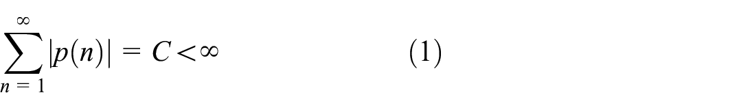
where C is a constant. While the correlations function p(n) is not absolutely summable for the LRD process first proposed by Hurst,²⁶ that is,

\sum_{n = 1}^{\infty} | p (n) | = \infty

(2)

The formula for sample mean variance of sample averages including n uncorrelated observations is

var (\bar{X}) = \frac{σ^{2}}{n}

(3)

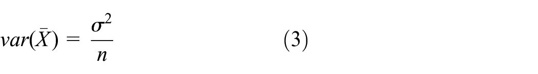
where X is the sample mean of sample averages, and σ is the standard deviation of sample observations, and n is sample size.

Besides, when the observations are correlated, that is, $\sum$ _i≠jp(i, j) ≠ 0, the expression of sample mean variance for sample average can be expressed as,

var (\bar{X}) = \frac{σ^{2}}{n} [1 + \frac{\sum i \neq jp (i, j)}{n}]

(4)

Obviously from the above equation (4), it can be seen that the LRD process is the tight bond between different time instants and slow decaying autocorrelation. Actually, there are common definitions that can be clarified to confirm the LRD process, given as below.

Definition 1: The condition that a stationary process can be regarded as having long-range correlation is its covariance function C(n) decaying tardily as n→∞, assuming the process has finite second-order statistics, that is, for 0 < α < 1

\lim_{n \to \infty} = \frac{C (n)}{n^{- α}} = c

(5)

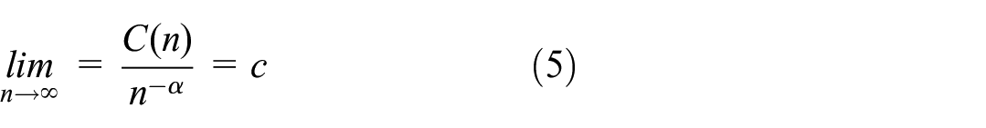
where c is a finite and positive constant. It means that C(n) can be equivalent to c/n^α for large n.²⁷ The parameter α = 2 − 2H, where H is the Hurst parameter.

Definition 2: As for weakly-stationary time-series X(t), it has the characteristic of long-range dependence if the corresponding spectral density meets

f (τ) = C_{f} {| τ |}^{- β}

(6)

as τ→ 0, for some C_f > 0 and some real parameters β∈ (0, 1). The parameter β is calculated by H = (1 + β)/2, which is relevant to Hurst parameter H.²¹

Based on these definitions, we will explore the phenomenon of LRD in machine acoustic signals in the following.

Exploitation of LRD in machine acoustics signal

LRD is usually associated with self-similar processes, the first and essential procedure in confirming whether there is long-range dependent in a given time series. Generally, it is difficult to accurately judge from the definition perspective, as its result is hard to figure out directly and might exist trend errors. From another aspect, LRD exhibits self-similarity characterized by the Hurst parameter H or H∈ (0.5, 1). Therefore, the degree of LRD can be represented by parameter H. Specifically, it obeys as following rules:

There is a greater persistence or long-range dependence with H closer to 1.

H = 0.5 corresponds to the lack of LRD.

H less than 0.5 means anti-persistency, opposite to L-RD, indicating a strong negative correlation and violent process fluctuation.

The parameter H can be operated using several methods, including rescaled range analysis, aggregated variance method, absolute value method, periodogram method, and local Whittle method. Many of them assume that the observation process is stationary, Gaussian, or at least linear. But the above assumption is often dissatisfactory in practice. Some estimation methods are impressionable to factors including data trends, data periodicity, and other corruption sources. Compared with those methods, aggregated variance method, absolute values method, and local Whittle method are good for SaS noise in robustness.²⁷ Meanwhile, aggregated variance method is simple and the calculation speed is the fastest. Therefore, the estimation for the parameter H of the observation series adopts aggregated variance method. For the given time series {Yt} with a length of N, it can be divided into sub-sequences of length of m. The mean value of each sequence is calculated by

Y_{k}^{(m)} = \frac{1}{m} \sum_{i = (k - 1) m + 1}^{k m} Y (i), k = 1, 2, \dots, [N / m]

(7)

For successive value of m in calculation, the estimate value of the sample variance of the sequence can be obtained by

\overset{\land}{{VarY}_{k}^{(m)}} = \frac{m}{N} \sum_{k = 1}^{N / m} (Y_{k}^{(m)} - E Y^{(m)})

(8)

For FGN and FARIMA processes, VarY^(m)−σ²m^β as m→∞, where σ is the scale parameter and β = 2H − 2. When N/m and m are large, asymptotic proportion is supposed to appear between sample variance VarY^(m) and m^2H−2, and a straight line with slope β = 2H − 2, β∈ (−1, 0), should be formed by the resulting points.²⁸ Based on the calculation of Hurst parameter, we can exploit the phenomenon of LRD for a given signal. Here, it is worth of mentioning that the importance of LRD in acoustics signals has been well accepted and recognized in wide-ranging areas, but it is not found in online monitoring of industrial machines based on acoustic signals. We therefore collected an original acoustics signal as shown in Figure 1(a) from our experimental setup that will be introduced in Section “Experimental setup and testing data,” and the give the computed Hurst parameter in Figure 1(b) where the result of H = 0.8979 reveals the great degree of long-range dependent hidden in the inspected machine acoustics signal. Here, it should also be noted that the LRD analysis of periodic signals may have some influence on the coefficient of LRD as shown in Figure 1(b), but it is able to be neglected in the LRD analysis of mechanical signals as discussed in Li et al.²⁰ and Li and Liang.²⁹ In the following, we will present the proposed framework that utilizes LRD for machine monitoring.

Figure 1.

Detection example of LRD on the inspected machine acoustic signal, where the speed was set as 50 rpm: (a) the collected original acoustics and (b) the LRD changes with time interval.

Proposed framework for online monitoring of industrial machine

Hereinafter, our algorithm will be proposed for real-time change detection in a data stream being monitored. We first overview the presented LRD model, subsequently, discuss techniques performed in the prediction steps. Finally, we shows the detection by using the residual error with adaptive change decision making. Methodologies used in the main steps are introduced and discussed, in the following.

Overview of the FARIMA prediction model

Different mathematical models can be used to define the so-called LRD with different application contexts and purposes. Among various models, the FARIMA (p, d, q) process is an effective and powerful tool to extract LRD for discrete-time processes,³⁰ where p is the autoregression order, d is the differencing order, and q is the moving average order. The values of p and q are non-negative integers, and d belongs to a non-integer (d∈ (−0.5, 0.5)).²⁸ A FARIMA (p, d, q) process X_t: t = …, −1, 0, 1, … is defined as

Φ (B) (1 - B)^{d} X_{t} = Θ (B) ε_{t}

(9)

where B is the backshift operator, defined by BX_t = X_t₋₁, {ε_t} is a white noise sequence.

Φ (B) = 1 - φ_{1} B - φ_{2} B^{2} \dots - φ_{p} B^{p}

(10)

Θ (B) = 1 + θ_{1} B + θ_{2} B^{2} \dots + θ_{p} B^{p}

(11)

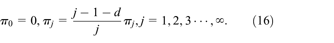
∇ = (1−B) is the differencing operator and ∇^d is the fractional differencing operator defined by

\nabla^{d} = (1 - B)^{d} = \sum_{k = 0}^{\infty} (\begin{matrix} d \\ k \end{matrix}) {(- B)}^{k}

(12)

where,

(\begin{matrix} d \\ k \end{matrix}) = \frac{Γ (d + 1)}{Γ (k + 1) Γ (d - k + 1)}

(13)

Γ denotes the Gamma function, which is defined by ∫^∞₀e^−tt^x−1dt, x > 0. Obviously, FARIMA (p, d, q) processes become the ARMA (p, q) processes in d = 0. The simplest form for FARIMA processes is FARIMA (0, d, 0) processes, and its property can describe long-range dependence like the fractional Gaussian model (FGN),²⁸ where the parameter d indicates the LRD strength, similar to the Hurst parameter H in FGN processes, H = d + 0.5.

Therefore, the FARIMA model can be separated into fractional differencing and ARMA model, where the key to achieve this separation is the fractional difference operator. Main steps are as follows:

Preprocess the collected data stream {Xt} for obtaining zero-mean time series {Yt}.

Estimate the Hurt parameter for long-range dependence analysis of the preprocessed data stream {Yt}.

Use the fractional differencing operator to do fractional differencing on series {Yt}.

Determine the parameters of ARMA model with minimum Alike information criterion (AIC) way.

Utilize the ARMA model with determined parameters to predict future data.

Perform the fractional integral filtering of parameter −d for the predicted data.

The specific prediction process is as shown in Figure 2.

Figure 2.

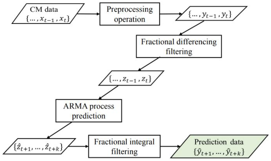
The flowchart of the proposed method.

Preprocess and estimate the hurst parameter

In order to adapt the model process and avoid interference resulted from different dimensions, data fluctuation, or significant difference in an observed data stream, we preprocess the data stream {Xt} with zero-mean value to get a sequence {Yt}.

As mention earlier, the fractional differencing operator is crucial to FARIMA model transformed into the relatively simple ARMA, where d is the important parameter. Due to d is equal to H– 0.5, the parameter H estimation are able to obtain the differing order d equivalently. The H is a self-similarity parameter, which represents LRD intensity in the time series, and its corresponding calculation have been explained in the previous section.

Fractional differential filtering

After obtaining the parameter d, we use the fractional differencing operator to filter the series {Y_t}. According to the equations (1) and (4), the expression as follows,

Z_{t} = \nabla^{d} Y_{t} = \sum_{k = 0}^{\infty} (\begin{matrix} d \\ k \end{matrix}) {(- B)}^{k} Y_{t} = \sum_{j = 0}^{\infty} π_{j} Y_{t - j}

(14)

where,

π_{j} = {(- 1)}^{j} \frac{Γ (d + 1)}{Γ (j + 1) Γ (d - j + 1)}

(15)

According to the recursive relation of the formula, the following relation can be obtained

π_{0} = 0, π_{j} = \frac{j - 1 - d}{j} π_{j}, j = 1, 2, 3 \dots, \infty .

(16)

For d < 0.5, the mean square of the above equation is convergence, thus the operator is complete. By this way, the series {Yt} with long-range dependence will transform into the series {Zt} with short-range dependence that conform to the ARMA model.

Figure 3 shows the hurst H of the series {Zt} after fractional differencing filtering and the hurst H is 0.277, which means the series has changed from LRD to SRD and conforms to the ARMA model process.

Figure 3.

Detection example of LRD based on sound signal in rotating machinery, where the speed is 50 rpm: (a) the collected original acoustics and (b) the LRD changes with time interval.

Parameter estimation on FARIMA mode

After fractional differencing filtering, the parameters estimation of FARIMA model can be equivalent to the parameters estimation of ARMA model in series {Zt}. Akaike information criterion (AIC), which is proposed by Akaike,³¹ can be used for determine the optimal parameters (p, q) of ARMA model. AIC is defined by

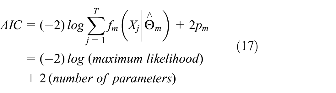
\begin{matrix} AIC = (- 2) \log \sum_{j = 1}^{T} f_{m} (X_{j} | \overset{\land}{Θ_{m}}) + 2 p_{m} \\ = (- 2) \log (\max imum likelihood) \\ + 2 (\begin{matrix} number of parameters \end{matrix}) \end{matrix}

(17)

When fitting the ARMA model with time series data, the gaussian likelihood can be regarded as real likelihood function, and the AIC can be rewritten as

A I C = (- 2) l o g {L (\overset{\land}{φ}, \overset{\land}{θ}, S (\overset{\land}{φ}, \overset{\land}{θ}) / T)} + 2 (p + q + 1)

(18)

where, $φ^{\land}$ and $θ^{\land}$ is the maximum likelihood estimators of {ϕ₁, …, ϕ_q} and {θ₁, …, θ_p}.

To validate the selected parameter model’s rationality, the autocorrelation function (ACF) and partial autocorrelation function (PACF) are analyzed for the residual error of the selected parameter model. Figure 4 is the ACF and PACF analysis for the model filtering residual of the aforementioned series after the ARMA model parameter estimation.

Figure 4.

ACF and PACF analysis of the model filtering residual: (a) ACF analysis and (b) PACF analysis.

Predict the data and perform the fractional integral filtering

We use the ARMA model to predict future multi-step time series $\overset{\land}{Z_{k}}$ . The actual predicted values $\overset{\land}{Y_{k}}$ can be obtained by fractional integral filtering, where the fractional differencing operator is ∇^−d.

Figure 5 shows the multi-step prediction data { $\overset{\land}{Y_{k}}$ , …, $\overset{\land}{Y_{k + 19}}$ }, which are generated by the aforementioned signal through the above process. From the picture, it is clearly seen that there is an excellent matched degree between predicted data in the FARIMA model and the actual data.

Figure 5.

Comparison prediction data with actual data.

Hypothesis testing based decision-making

The residual analysis is performed between the prediction data $\overset{\land}{Y_{k}}$ and the real observed data Y_k, the residual error can be obtained by

s_{k} = \overset{\land}{Y_{k}} - Y_{k}

(19)

Aiming to detect whether there is a change taken place at the current time point, a 3σ control chart assuming Gaussian distribution is adopted for the hypothesis testing based on the residual analysis.

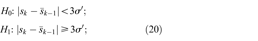
\begin{matrix} H_{0} : | s_{k} - {\bar{s}}_{k - 1} | < 3 σ'; \\ H_{1} : | s_{k} - {\bar{s}}_{k - 1} | \geq 3 σ'; \end{matrix}

(20)

where H₀ indicates that if |s_k− ${\bar{s}}_{k - 1}$ | < 3σ′, there is unchanged on the time point k. H₁ represents a change appearing when |s_k− ${\bar{s}}_{k - 1}$ | ≥ 3σ′. Here, ${\bar{s}}_{k - 1}$ and σ′ are the mean and standard deviation of the Gaussian distribution respectively, and calculated by

{\bar{s}}_{k - 1} = \frac{1}{k - 1} \sum_{j = 1}^{k - 1} s_{j}

(21)

σ = \sqrt{\frac{1}{k - 1} \sum_{j = 1}^{k - 1} {(s_{j} - {\bar{s}}_{k - 1})}^{2}}

(22)

It’s noteworthy that the change points maybe detected from two aspect: abnormal state or random noises.³² An adaptive detection method is proposed to suppress random noise effects. That is to say, the anomalous point judged by r + 1 consecutive residuals waiting for detection is regarded as the real change point. The detection process is described as follows:

First, when the change point is detected firstly, the change point k is noted by C₀, setting r = 0.

Second, letting r = r + 1, and searching for the change point k, the point k is noted by C_r when the consecutive r + 1 residual error values {s_k_+m}_m=0:r satisfy {|s_k_+m− ${\bar{s}}_{k - 1}$ |≥3σ′}_m=0:r.

Third, let r increases from 1 until r satisfies C₀ = C_r, and output C_r as the real change point.

The stability of the C_r improves as r increases, implying a well-inhibiting effect for state change resulting from random noises.

Experiment

This section validates the proposed framework based on our experimental setup, and meanwhile compares it with cutting-edge methods.

Experimental setup and testing data

The experimental facility to collect testing data is shown in Figure 6, which power is provided by an three-phase alternating-current motor with rated power of 0.75 kW and rated voltage of 230 V. The vibration signals, 1000 Hz sampling frequency, are collected by a sound sensor installed on the gear box, and transmitted to PC subsequently. The reason for selecting acoustic signal as a condition monitoring index is the advantage of immediacy, non-invasive, and low cost.³³

Figure 6.

Experimental setup for collection of testing data: (a) front view and (b) schematic.

In the process of data acquisition, the motor operates at an initial speed ν, varying at an interval of Δν to simulate speed change conditions (i.e. ν→ν + Δν). The conditions set as follows,

ν {50, 100, 150, 200, 250} rpm;

Δν {50, 100, 150, 200, 250} rpm.

There are 24 conditional combinations of speed change, as shown in Table 1. The proposed method is the ARIMA model³⁴ which does not have the characteristics of describing LRD and the graph model¹² which has the ability to depict the LRD property to some extend. In the following experiments, the first detected alarm determines whether the detection is successful or false. Then the detection performance is quantified by a precision indicator defined as the ratio of the number of correctly detected changes over the total number of changes.

Table 1.

Simulated speed condition change ν→ν + Δν (rpm).

Δν\ν	50	100	150	200	250
50	50 → 50 + 50	100 → 100 + 50	150 → 150 + 50	200 → 200 + 50	250 → 250 + 50
100	50 → 50 + 100	100 → 100 + 100	150 → 150 + 100	200 → 200 + 100	250 → 250 + 100
150	50 → 50 + 150	100 → 100 + 150	150 → 150 + 150	200 → 200 + 150	250 → 250 + 150
200	50 → 50 + 200	100 → 100 + 200	150 → 150 + 200	200 → 200 + 200	250 → 250 + 200
250	50 → 50 + 250	100 → 100 + 250	150 → 150 + 250	200 → 200 + 250	250 → 250 + 250
300	50 → 50 + 300	100 → 100 + 300	150 → 150 + 300	200 → 200 + 300	250 → 250 + 300
350	50 → 50 + 350	100 → 100 + 350	150 → 150 + 350	200 → 200 + 350	250 → 250 + 350

Result and analysis

Figure 7 shows the change detection result on the test data, of which the speed change is from 50 to 150 rpm performed manually. From top to bottom, it shows the original signal data, the prediction value and the detection results based on residual error, respectively. It is observed that the prediction values can accurately reflect the structure trend of the original signal because of the LRD of FARIMA model. Meanwhile, the residual error shows high prediction accuracy and a remarkable increase at the change time such that the change was detected successfully. To further elucidate the predictive ability of LRD model in machine condition monitoring, a local magnification of the aforementioned example is shown in Figure 8. The overlap figure of actual and predicted signals, residual error, local magnification of segment (1) and (2) of the overlap figure are displayed in Figure 8 from top to bottom respectively. It is obviously seen that the prediction signal resembles the actual signal in the local magnification picture of segment (1). At the change time, the predicted data is obviously different from the actual data as shown in Figure 8(b).

Figure 7.

An example of change detection for speed change from 50 to 150 rpm: (a) the original signal, (b) the prediction value, and (c) the detection results based on residual error.

Figure 8.

The overlap degree of actual and predicted signals, residual error: (a) overall situation and (b) local magnification of segment.

Figure 9 shows an example of change detection for three comparison methods, where the speed varies from 50 to 150 rpm and the change point is marked by a instructor. The subfigure (a) shows detection result based on the graph model method, in which the original signal data and the detection results based on anomaly score from top to bottom, respectively. In sub-figure (b) and (c), from top to bottom, the original signal data, the prediction value, and the detection results based on residual error are displayed separately. It serves to show that only the proposed method can accurately detect the change point, while no alarm points were detected in the ARIMA model and the graph model. The main reason is ARIMA model only capture the SRD and graph model has the ability to describe the LRD property to some extend.

Figure 9.

Comparison results with different models: (a) graph model, (b) ARIMA model, and (c) FARIMA model.

We also compared the proposed method with the ARIMA model and graph-based method reported in Lu et al.^12,34 as they have been demonstrated outperforming results than typical methods including mean, RMS, kurtosis, and skewness. Table 2 gives the comparison results and shows that the detection performance of the proposed method is superior to the compared methods, which reveals good potentials of the proposed framework in practical engineering applications.

Table 2.

Comparison results.

Δν\v	Our method					ARIMA model					Graph model
	50	100	150	200	250	50	100	150	200	250	50	100	150	200	250
50	✓	✓	✓	✓	x	x	✓	✓	✓	x	✓	✓	✓	✓	x
100	✓	✓	✓	✓	✓	x	✓	x	✓	x	✓	✓	x	✓	x
150	✓	✓	✓	✓	✓	x	✓	✓	✓	x	✓	✓	x	✓	✓
200	✓	✓	✓	✓	✓	x	✓	x	✓	x	✓	✓	x	✓	x
250	✓	✓	✓	✓	✓	x	✓	x	✓	x	✓	✓	x	✓	✓
300	✓	✓	✓	✓	✓	x	x	x	x	x	✓	✓	x	✓	x
350	✓	✓	✓	✓	✓	x	✓	x	✓	x	✓	✓	x	✓	✓
Precision	34/35					14/35					25/35

Conclusion

Acoustics signal is common in online monitoring of industrial machines. This paper suggests the exploitation of LRD from continuously-collected acoustics signals in order to detect early changes of rotational speed for considered machines. To achieve this end, a new unified framework is developed in this paper. In the framework, FARIMA is adopted to extract predicted value of LRD as the judgment index of state change, and decision-making based on null hypothesis test is used to detect the change point. The comparison between the predicted data and the actual data shows that FARIMA has good accuracy for LRD prediction. The results of comprehensive experiments show that this framework is outperforming the state-of-the-arts, and demonstrate good potentials of the proposed framework in real engineering applications. In the future, we will optimize the algorithm to achieve a higher computational efficiency, and apply it for practical applications.

Footnotes

Handling Editor: Aarthy Esakkiappan

Declaration of conflicting interests

The author(s) declared no potential conflicts of interest with respect to the research, authorship, and/or publication of this article.

Funding

The author(s) disclosed receipt of the following financial support for the research, authorship, and/or publication of this article: This work is supported by the Natural Science Foundation of Hubei Province of China under Grant No. 2019CFC909.

ORCID iD

Guoliang Lu

References

Chen

Zhao

Kim

, et al. Wheel fault diagnosis model based on multichannel attention and supervised contrastive learning. Adv Mech Eng 2021; 13: 16878140211067024.

Kawano

Hattori

Takeda

, et al. Early structural change detection as an optimal stopping problem: solution theorem and its proof using reduction to absurdity. Artif Life Robot 2010; 15: 425–430.

Lin

C-L

Liang

J-W

Huang

Y-M

, et al. A novel model-based unbalance monitoring and prognostics for rotor-bearing systems. Adv Mech Eng 2023; 15: 16878132221148019.

Peng

Dong

Zuo

MJ.

Current status of machine prognostics in condition-based maintenance: a review. Int J Adv Manuf Technol 2010; 50: 297–313.

Chen

Jiang

Ding

, et al. Data-driven fault diagnosis for traction systems in high-speed trains: a survey, challenges, and perspectives. IEEE Trans Intell Transp Syst 2022; 23: 1700–1716.

Gougam

Afia

Aitchikh

, et al. Computer numerical control machine tool wear monitoring through a data-driven approach. Adv Mech Eng 2024; 16: 16878132241229314.

Guo

An integrated approach for bearing health indicator and stage division using improved Gaussian mixture model and confidence value. IEEE Trans Industr Inform 2022; 18: 5219–5230.

Kruger

Lamont

, et al. Fault detection in non-Gaussian vibration systems using dynamic statistical-based approaches. Mech Syst Signal Process 2010; 24: 2972–2984.

Ahmad

Khan

Islam

, et al. A reliable technique for remaining useful life estimation of rolling element bearings using dynamic regression models. Reliab Eng Syst Saf 2019; 184: 67–76.

10.

Cheng

A comprehensive review and comparison of CUSUM and change-point-analysis methods to detect test speededness. Multivariate Behav Res 2022; 57: 112–133.

11.

Antoni

Borghesani

A statistical methodology for the design of condition indicators. Mech Syst Signal Process 2019; 114: 290–327.

12.

Liu

Yan

Graph-based structural change detection for rotating machinery monitoring. Mech Syst Signal Process 2018; 99: 73–82.

13.

Cheng

Wang

Meng

, et al. Sigma-mixed unscented Kalman filter-based fault detection for traction systems in high-speed trains. Chin J Electron 2023; 33: 1–10.

14.

Liu

Application of BP and AR model in performance degradation assessment and prediction of bearings. J Electron Meas Instrum 2019; 33: 79–88.

15.

Stavropoulos

Papacharalampopoulos

Souflas

Indirect online tool wear monitoring and model-based identification of process-related signal. Adv Mech Eng 2020; 12: 1687814020919209.

16.

Long

Wang

, et al. Applications of fractional lower order frequency spectrum technologies to bearing fault analysis. Math Probl Eng 2019; 2019: 7641383.

17.

Yi-ze

Qing-tang

State prediction of MR system by VMD-GRNN based on fractal dimension. Adv Mech Eng 2022; 14: 16878132221145899.

18.

Sun

Zhou

Xiang

, et al. Hankel matrix-based condition monitoring of rolling element bearings: an enhanced frame-work for time-series analysis. IEEE Trans Instrum Meas 2021; 70: 1–10.

19.

Tena García

Cadenas Calderón

González Ávalos

, et al. Forecast of daily output energy of wind turbine using sARIMA and nonlinear autoregressive models. Adv Mech Eng 2019; 11: 1687814018813464.

20.

Liang

Yang

, et al. Long range dependence prognostics for bearing vibration intensity chaotic time series. Entropy 2016; 18: 23.

21.

Mccormick

Nandi

AK.

Cyclostationarity in rotating machine vibrations. Mech Syst Signal Process 1998; 12: 225–242.

22.

Cha

Yoo

Lee

, et al. Classification of acoustic noise signals using wavelet spectrum based support vector machine. J Mech Sci Technol 2018; 32: 2453–2462.

23.

Kan

Tan

Mathew

A review on prognostic techniques for non-stationary and non-linear rotating systems. Mech Syst Signal Process 2015; 62: 1–20.

24.

Assadhan

Zeb

Al-Muhtadi

, et al. Anomaly detection based on LRD behavior analysis of decomposed control and data planes network traffic using SOSS and FARIMA models. IEEE Access 2017; 5: 13501–13519.

25.

Lin

Jiang

Lai

, et al. A new algorithm on lagged correlation analysis between time series: TPFP. J Comput Res Dev 2012; 12: 2645–2655.

26.

Hurst

HE.

Long-term storage capacity of reservoirs. Trans Am Soc Civil Eng 1951; 116: 770–799.

27.

Sheng

Chen

FARIMA with stable innovations model of Great Salt Lake elevation time series. Signal Process 2011; 91: 553–561.

28.

Sheng

Chen

Qiu

Fractional processes and fractional-order signal processing: techniques and applications. New York, NY: Springer Science & Business Media, 2011.

29.

Liang

Degradation trend prediction for rotating machinery using long-range dependence and particle filter approach. Algorithms 2018; 11: 89.

30.

Brockwell

Davis

Fienberg

SE.

Time series: theory and methods. New York, NY: Springer Science & Business Media, 1991.

31.

Akaike

Factor analysis and AIC. Psychometrika 1987; 52: 317–332.

32.

Lei

Jing

, et al. An improved exponential model for predicting remaining useful life of rolling element bearings. IEEE Trans Ind Electron 2015; 62: 7762–7773.

33.

Glowacz

Fault diagnosis of single-phase induction motor based on acoustic signals. Mech Syst Signal Process 2019; 117: 65–80.

34.

Zhou

, et al. A novel framework of change-point detection for machine monitoring. Mech Syst Signal Process 2017; 83: 533–548.

Exploitation of long-range acoustic dependence for early change detection in dynamic machine running status

Abstract

Keywords

Introduction

Overview of this paper

Structure for the rest of this paper

Long-range dependence (LRD) in acoustics signals

The LRD phenomenon

Exploitation of LRD in machine acoustics signal

Proposed framework for online monitoring of industrial machine

Overview of the FARIMA prediction model

Preprocess and estimate the hurst parameter

Fractional differential filtering

Parameter estimation on FARIMA mode

Predict the data and perform the fractional integral filtering

Hypothesis testing based decision-making

Experiment

Experimental setup and testing data

Result and analysis

Conclusion

Footnotes

Declaration of conflicting interests

Funding

ORCID iD

References