Analysis and simplified model calculation of residual stress in U-rib welding of steel bridge deck

Abstract

This article examines residual stress generation in U-ribbed steel bridge deck during welding, focusing on post-welding changes in the base material’s residual stress pattern. A thermo-elasto-plastic finite element analysis model was established to conduct numerical simulations of the welding process, summarizing the residual stress changes near the weld seam, the conclusion was drawn that the tensile and compressive forms of transverse residual stress on the upper and lower surfaces of the base plate were inconsistent. To validate the proposed numerical simulation method’s accuracy, the blind hole method was employed to measure welding-induced residual stress, and finite element analysis calculated calibration coefficients A and B, demonstrating the method’s effectiveness. Comparison of experimental measurements with numerical simulation outcomes validate the finite element simulation method’s accuracy and the adopted methodology’s feasibility. Based on these findings, a piecewise linear fitting approach was adopted to develop a simplified model of welding residual stress. The simplified model provides the initial conditions of residual stress for mechanical calculation of U-rib of the same type.

Introduction

Currently, steel bridge deck construction heavily relies on on-site welding techniques. The welding process generates residual stresses due to uneven temperature fields and resultant local plastic deformation, directly affecting the load-bearing capacity and durability of steel bridge deck. Residual stresses, exacerbated by temperature and medium, significantly ¹ impair the weld joints’ resistance to brittle fracture, stress corrosion cracking, high-temperature creep cracking, affecting fracture characteristics and fatigue strength. ² Thus, it is essential to emphasize the importance of welding residual stress distribution for the reliable design of welded structures. Numerous scholars have conducted detailed simulations and experimental studies on welding residual stresses. Kainuma et al. ³ compared residual stress distributions against both experimental and finite element analysis results. Additionally, Banik et al. ⁴ conducted thermal analyses with real welding parameters and temperature-dependent material properties, generating temperature curves for comparison with measured values. Park et al. ⁵ investigated the effects of member thickness, yield stress, lateral constraint, and bending constraint on the welding residual stress in butt welding and established predictive factors for welding residual stress. Recently, Hossain et al. ⁶ conducted finite element analysis on DHD (deep hole drilling method), showing that elastoplastic analysis with an incremental method could more accurately reconstruct initial in-plane residual stresses, though it overestimated out-of-plane stresses. Pandey et al. ⁷ measured the angular deformation of 12 mm thick double-sided fillet welding in positive and negative direction, and concluded that the maximum angular deformation of reverse fillet welding was small. Cui et al. ⁸ measured the initial welding residual stress of the welded joints of the deck by ultrasonic method, and simulated it using a sequential coupled thermo-mechanical finite element model. The model was verified by the test data and used for the analysis of welding residual stress relaxation. Gu et al. ⁹ explored the magnitude and distribution of the residual stress in the welding of orthotropic steel with U-shaped ribs, used the thermoelastoplastic finite element method to simulate the residual stress of welding, and finally measured the residual stress by the borehole strain gauge method. Taraphdar et al. ¹⁰ discovered a new method for measuring residual stress through thickness based on general strain relaxation, combined with traditional deep hole drilling techniques and the new contour method, which reduces the degree of damage to components during measurement. Sauraw et al. ¹¹ performed a profile butt weld on a conventional V-groove design and performed microstructure characterization of the welded joint to measure the heterogeneity of its microstructure and the diffusion of elements across the interface. Liang et al. ¹² studied the distribution of welding residual stress of single-sided and full-penetration double-sided U-ribs, and conducted numerical and experimental studies considering different deck thicknesses. Kollár et al. ¹³ established the first residual stress model of orthotropic U-shaped steel bridge deck based on residual stress measurement results, and the proposed simplified residual stress model is suitable for the welding of single-groove steel structures with S355 and below steel grades.

Analysis of welding model of U-rib and base plate

Thermophysical property definition

The welding process belongs to a nonlinear change process. ¹⁴ At the same time, it is necessary to define the material elastic modulus, yield stress, thermal expansion coefficient and stress-strain strengthening of the structure at different temperatures. In this paper, Q355D low carbon alloy steel is intended to be used for simulation and analysis of the steel bridge deck material parameters of Xiangshan Bridge. The thermophysical properties of Q355D ¹⁵ low carbon alloy steel at different temperatures are shown in Table 1.

Table 1.

At elevated temperature physical parameter properties of Q355D low alloy steel.

Temp./ $°\mathrm{C}$	Thermal conductivity/ $\mathrm{W}·(\mathrm{m}·°\mathrm{C}{)}^{-1}$	Specific-heat capacity/ $\mathrm{J}·(\mathrm{kg}·°\mathrm{C}{)}^{-1}$	Heat transfer coefficient/ $\mathrm{W}·({\mathrm{m}}^2·°\mathrm{C}{)}^{-1}$	Thermal expansion coefficient/ $(\times {10}^5/°\mathrm{C})$	Elastic modulus/GPa	Possion’s ratio	Yield stress/MPa
20	51.9	450	55	1.095	206	0.28	375
500	37.5	705	39	1.352	150	0.36	178
700	31.4	1028.8	84	1.410	70	0.37	40
1100	29.5	418.5	150	1.462	20	0.37	2
1500	29.7	400	264	1.600	19	0.42	2

Welding heat source input definition

Selecting a suitable welding heat source model and accurately determining the values of parameters in the model are very important for the simulation of welding temperature field, and are also the prerequisite for obtaining more accurate welding residual stress and deformation.

Rosenthal ¹⁶ simplified heat sources into point, line and plane heat sources according to different shapes of welds, and gave the analytical formula of the transient temperature field under each heat source. Since the heat source models proposed by the authors are all concentrated heat sources, and the thermophysical parameters of the materials are assumed to be unchanged, the calculated results are only valid for the low temperature zone away from the weld, and the prediction accuracy of the temperature in the weld zone is poor, which is the most concerned area of the welding temperature field and stress field. Eagar and Tsai ¹⁷ improved Rosenthal D’s theory and proposed a 2D planar Gaussian heat source model, which could predict the temperature field in the near seam zone. However, this heat source model could not consider the influence of penetration depth, and was only applicable to the situations where thin plate penetration welding or arc stiffness (the degree of arc rigidity along the electrode axis) was small. To solve this problem, Goldak et al. ¹⁸ proposed a double ellipsoidal heat source model (DEHSM) that considered the effect of searing. In this model, the front and back two quarter ellipsoids were used to simulate the energy density distribution of the heat source. The heat flux function of the front ellipsoidal is as follows:

$$q_f=\frac{\left(6\sqrt{3}{f}_{1}Q\right)}{\left(\pi a_f\mathrm{bc}\sqrt{\pi }\right)}\exp \left(\frac{-3x^2}{\left(a_f^2\right)}\right)\exp \left(\frac{-3y^2}{b^2}\right)\exp \left(\frac{-3z^2}{c^2}\right)$$

(1)

$$q_r=\frac{\left(6\sqrt{3}{f}_{2}Q\right)}{\left(\pi a_r\mathrm{bc}\sqrt{\pi }\right)}\exp \left(\frac{-3x^2}{\left(a_r^2\right)}\right)\exp \left(\frac{-3y^2}{b^2}\right)\exp \left(\frac{-3z^2}{c^2}\right)$$

(2)

Where, $Q=\eta \mathrm{UI}$ , $\eta$ is the efficiency, $U$ is the voltage, $I$ is the current, $f_1$ and $f_2$ are the front and back parameters and satisfy $f_1$ + $f_2$ =2, $a_f,a_r,b,c$ are the shape parameters of the ellipsoid, respectively.

In this article, the double ellipsoid model is used to apply heat source and simulate the calculation. In this article, the parameter v = 5 mm/s, U = 630 V, I = 30 A, f₂ = 2f₁, $a_f$  = b = 5 mm, $a_r$  = 10 mm, c = 7.2 mm.

Thermal cycle curve of welding process

The finite element software MSC-Marc 2020 was selected to simulate and analyze the welding. In this paper, SOLID70 solid element is used for thermal-structural coupling analysis. In order to make the calculation more rapid, the welding filler is the same material as the base metal. The weld is activated according to the actual welding speed in the model. The air convection boundary is added to the structure by thermal analysis, and the structure analysis boundary is in the form of constraint on the four corners of the bottom plate.

Figure 1 shows the temperature field of the welding section of the cladding welding outside the U rib. By analyzing the shape of the molten pool and comparing it with the actual weld shape, it can be concluded that the simulated melting part is close to the actual melting part, and the welding heat source is applied reasonably.

Figure 1.

Temperature cloud image of weld pool shape. (a) Weld pool, (b) weld shape.

The temperature change of the measuring point in the whole simulation process can be extracted, and the temperature change of different positions in the weld with time can be obtained after processing the time history. Figure 2(a) and (b) respectively show the positions of five temperature measurement points and the thermal cycle curves.

Figure 2.

Heat cycle curve at each point along the weld direction. (a) Temperature measuring point location and (b) temperature thermal cycle curve.

As can be seen from Figure 2(b), the temperature of each measuring point on the welded component changes with the change of welding time, and the temperature is unstable at the beginning of welding. Along the welding direction, each measuring point moves with the heat source to heat the welding in turn. With the departure of the heat source, the temperature dropped rapidly. After 200 s, the temperature of the five measuring points all dropped below 200°C, and then gradually flattened. As the cooling process continues, the temperature of each measuring point drops and gradually approaches room temperature.

Analysis of welding residual stress in welding center section

Equivalent residual stress analysis

After the end of welding, the residual stress of the member can be regarded as evenly distributed along the weld, ¹⁹ ignoring the influence of the arc section and the arc section, and selecting the welding equivalent residual stress of the base plate at the center section where the welding path is relatively stable for analysis. Figure 3 shows the equivalent Mises welding residual stress distribution nephogram. Figure 4(a) and (b) show the distribution of equivalent Mises welding residual stress on the upper surface and lower surface of the stiffener base plate of U-shaped bridge panel.

Figure 3.

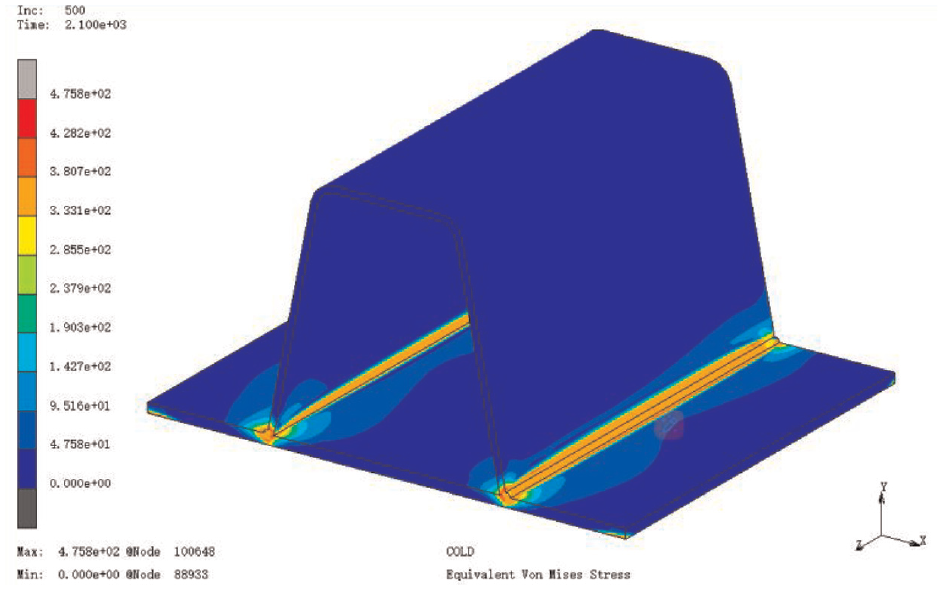
Equivalent Mises welding residual stress distribution nephogram.

Figure 4.

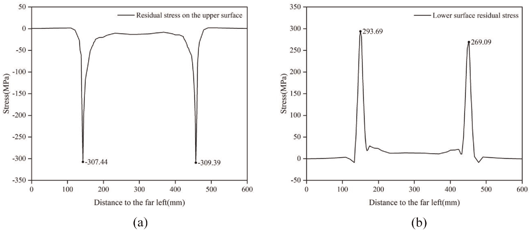
Equivalent Mises residual stress distribution of the base plate. (a) Equivalent Mises residual stress distribution on the upper surface and (b) lower surface equivalent Mises residual stress distribution.

As can be seen from Figure 4(a) and (b), the equivalent residual stress on both sides of the mother plate is symmetrically distributed, and the maximum welding residual stress on the upper and lower surfaces is close to the yield strength. The equivalent residual stress value is the largest in the weld and near-weld areas, including the position of the base plate near the weld. Among them, the equivalent residual stress of the base plate begins to drop sharply within the range of both sides of the weld at 10mm from the weld center, that is, about two times the width of the weld (5 mm). And at 16 mm from the weld center, that is, about three times the thickness of the weld width (5 mm) on both sides of the weld to the lowest value, then the stress change tends to be flat.

Residual stress analysis of base plate

In addition to the analysis of the equivalent residual stress of the mother board, it is also necessary to analyze the lateral and longitudinal residual stress of the mother board. The extraction path of the residual stress and the overall coordinates are shown in Figure 5. Figure 6 shows the transverse welding residual stress nephogram and Figure 7 shows the longitudinal welding residual stress nephogram The residual stress σx distribution diagram of the base plate along the path is shown in Figure 8(a) and (b). Figure 9(a) and (b) show the residual stress σz distribution diagram of the base plate along the path.

Figure 5.

Stress extraction path diagram.

Figure 6.

Transverse welding residual stress nephogram.

Figure 7.

Longitudinal welding residual stress nephogram.

Figure 8.

The residual stress $\mathrm{\sigma }x$ distribution diagram of the base plate along the path. (a) Distribution of residual stress σx along the path on the upper surface and (b) distribution of residual stress σx along the path on the lower surface.

Figure 9.

The residual stress $\sigma z$ distribution diagram of the base plate along the path. (a) Distribution of residual stress σz along the path on the upper surface and (b) distribution of residual stress σz along the path on the lower surface.

The base plate’s surface predominantly exhibits transverse residual stresses in a compressive state. Figure 8(a) shows that residual stress values peak at approximately 0.78 times the material’s yield strength, about 7 mm from the weld center. In the weld’s heat-affected zone, stress spans about 30 mm, with minimal stress values across the rest of the base plate. Conversely, the base plate’s underside predominantly displays transverse residual stresses in a tensile state.

Figure 8(b) indicates the peak transverse residual tensile stress directly beneath the weld center is about 0.75 times the yield strength, with an abrupt change in tensile stress over approximately 35 mm. Between two welds, the base plate exhibits a tensile stress of approximately 12 MPa, diminishing towards the center, while the sides show lower stress values with minor compressive stress near the welds.

Figure 9(a) demonstrates that the base plate surface near the weld exhibits tensile stress, flanked by compressive stress on either side. Near the weld, residual tensile stress peaks about 3 mm from the center, exceeding the material’s yield strength by approximately 1.17 times. Within 30 mm on both sides of the weld, residual tensile stress sharply declines and transitions to compressive stress around one times the rib plate thickness (12 mm) from each side. The peak of residual compressive stress is found 15 mm from the weld center, with the maximum value about 0.21 times the yield strength.

Figure 9(b) shows the base plate’s underside near the weld has a similar stress distribution to the top, with tensile stress flanked by compressive stress on both sides. The residual tensile stress near the weld is considerable, with a peak value about 3 mm from the center, around 0.77 times the yield strength. Over a 25 mm range on either side of the weld, residual tensile stress declines sharply and transitions to compressive stress approximately 8 mm from each side. The peak of residual compressive stress is about one time the rib plate thickness (12 mm) from the center, with the maximum value approximately 0.21 times the yield strength. Apart from the peak values exceeding the material’s yield strength, the remaining stress characteristics and trends closely resemble those on the top surface (Figure 10).

Figure 10.

Blind-hole method residual stress test strain gage rosettes.

Welding residual stress experiment

Basic principle of blind hole experiment

According to Kirsch ²⁰ formula, ${\epsilon }_1$ , ${\epsilon }_2$ , ${\epsilon }_3$ can be expressed as:

$$\begin{array}{c}{\epsilon }_1=A({\sigma }_1+{\sigma }_2)+B({\sigma }_1-{\sigma }_2)\cos 2\beta \hfill \\ {\epsilon }_2=A({\sigma }_1+{\sigma }_2)+B({\sigma }_1-{\sigma }_2)\cos 2(\beta +45°)\hfill \\ {\epsilon }_3=A({\sigma }_1+{\sigma }_2)+B({\sigma }_1-{\sigma }_2)\cos 2(\beta +90°)\hfill \end{array}$$

(3)

$$\beta =\frac{1}{2}{\tan }^{-1}\left(\frac{{\epsilon }_1-2{\epsilon }_2+{\epsilon }_3}{{\epsilon }_3-{\epsilon }_1}\right)$$

(4)

In the formula, ${\sigma }_1$ and ${\sigma }_2$ are the main stresses; $\beta$ main stress direction angle (abbreviated “direction angle”); A and B are strain release coefficients. The various parameters of BF-120-1 strain height rosettes are shown in Figure 10.

By writing the formula (3) as ${\sigma }_1$ , ${\sigma }_2$ for ${\epsilon }_1$ , ${\epsilon }_2$ , ${\epsilon }_3$ , the formula for calculating stress from strain can be obtained, such as:

$${\sigma }_{1,2}=\frac{1}{4A}({\epsilon }_1+{\epsilon }_3)\mp \frac{1}{4B}\sqrt{{({\epsilon }_3-{\epsilon }_1)}^2+{({\epsilon }_1+{\epsilon }_3-2{\epsilon }_2)}^2}$$

(5)

The released strain measured by the borehole can be substituted into the formula to calculate the maximum and minimum principal stresses. The stress direction is converted by the stress circle. The stress is mainly determined by the release coefficient of A and B. If the material changes within the range of linear elasticity, the coefficients A and B obtained by the calculation formula of Kirsch theory can be expressed as:

$$\begin{array}{c}A=-\frac{1+\mu }{2E}\frac{a^2}{r_1{r}_2}\hfill \\ B=-\frac{1}{E}\frac{2a^2}{r_1{r}_2}[1-\frac{1+\mu }{4}\frac{a^2(r_1^2+r_1{r}_2+r_2^2)}{r_1^2{r}_2^2}]\hfill \end{array}$$

(6)

Where $E$ and $\mu$ are the elastic modulus and Poisson’s ratio of the material; $a$ is the radius of the hole; $r_1$ and $r_2$ are the distance between the center of the circular hole and the near end and far end of the strain grid respectively.

Calibration coefficients A and B can be calibrated not only by finite element method, but also by experimental method. In the experiment, stress ${\sigma }_1$ and ${\sigma }_2$ are applied to the specimen, and then strain ${\epsilon }_1$ , ${\epsilon }_2$ and ${\epsilon }_3$ caused by drilling are tested, and then the expression of A and B can be obtained by substituting into equation (5), as shown in equation (7).

If a unidirectional stress is applied ${\sigma }_1$ =  $\sigma$ , ${\sigma }_2$  = 0. The 1# strain gauge is pasted along the direction of ${\sigma }_1$ , and formula 1 and 3 of formula (4) are substituted to obtain the expressions of the uniaxial stress calibration coefficients A and B, as shown in formula (8).

$$\begin{array}{c}A=\frac{{\epsilon }_1+{\epsilon }_3}{2({\sigma }_1+{\sigma }_2)}\hfill \\ B=\frac{\sqrt{{({\epsilon }_3-{\epsilon }_1)}^2+{({\epsilon }_1+{\epsilon }_3-2{\epsilon }_2)}^2}}{2({\sigma }_2-{\sigma }_1)}\hfill \end{array}$$

(7)

$$\begin{array}{c}A=\frac{{\epsilon }_1+{\epsilon }_3}{2\sigma }\hfill \\ B=\frac{{\epsilon }_1-{\epsilon }_3}{2\sigma }\hfill \end{array}$$

(8)

BF-120-1 strain gage rosettes is intended to be used for testing welding residual stress in this article. JD2-16E magnetic base drilling, drilling diameter and depth are 2.0 mm; Strain measurement using JM8813 static strain measurement system shown in the Table 2.

Table 2.

Strain gage rosettes specification size (mm).

Parameter	r	$r_1$	$r_2$	d	a
Dimensions	2.5	1.5	3.5	2	1

A, B coefficient finite element method calibration

Establishment of calibrated finite element model

The calibrated finite element model of A and B coefficients is shown in Figure 11. The simulated force and deformation are symmetrical structures. In order to reduce the calculation amount, 1/4 is selected for modeling. The size of the model is 50 mm × 50 mm × 10 mm, and the displacement constraints of X = 0 and Y = 0 are applied to the symmetric section, and the vertical Z-body displacement of the structure is limited. Figure 12 shows the division of units near the blind holes. The sensitive grilles are divided by 0.5 mm for accurate structural calculation

Figure 11.

Model diagram.

Figure 12.

Blind hole and nearby element division.

In this article, the drilling part is divided into eight layers by using the birth-and-death technique of Ansys Workbench 2022 to simulate the drilling process. The C3D8R type solid unit is selected by the software, and the material properties are selected according to the actual steel. The first layer is 0.25 mm, and the drilling diagram is shown in Figure 13. During calculation, the 8-layer element is killed, and the final finished state is shown in Figure 14.

Figure 13.

Drilling process diagram.

Figure 14.

Drilling completion diagram.

The finite element simulation of A and B calibration coefficients sets nine loading steps. The first step applies principal stress ${\sigma }_1$ and ${\sigma }_2$ to simulate the initial residual stress state. The stress forms of ${\sigma }_1$ and ${\sigma }_2$ are added in an equivalent way to the boundary stress, with pull as the positive direction and pressure as the negative direction. In the next few steps, the entire drilling process is simulated according to the stage of “killing” the 8-layer unit in the blind hole area.

Assumes that the stress of 1 #, 2 #, 3 # strain gauge reading respectively ${\epsilon }_1\prime$ , ${\epsilon }_2\prime$ , ${\epsilon }_3\prime$ , after the completion of the borehole readings for the ${\epsilon }_1″$ , ${\epsilon }_2″$ , ${\epsilon }_3″$ , in the initial stress ${\sigma }_1$ , ${\sigma }_2$ , released by the borehole strain ${\epsilon }_1$ , ${\epsilon }_2$ , ${\epsilon }_3$ as follows:

$$\begin{array}{c}{\epsilon }_1={\epsilon }_1″-{\epsilon }_1\prime \hfill \\ {\epsilon }_2={\epsilon }_2″-{\epsilon }_2\prime \hfill \\ {\epsilon }_3={\epsilon }_3″-{\epsilon }_3\prime \hfill \end{array}$$

(9)

Calculation of calibration coefficient in finite element

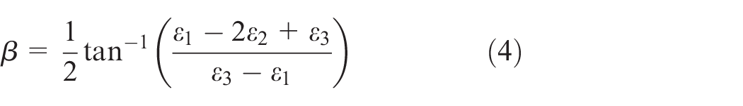
The 120° strain rosette depends on the extension or shortening of the sensitive grid to measure the strain, so the strain corresponding to the reading of the strain gauge can be extracted by the change of the length of the center line of the sensitive grid in the finite element calculation result. As shown in Figure 15, $\overline{P_{11}{P}_{12}}$ , $\overline{P_{21}{P}_{22}}$ , and $\overline{P_{31}{P}_{32}}$ are the centerline lengths of the sensitive grid of the 1#, 2#, and 3# strain gauges. The following takes 1# strain gauge as an example to introduce the extraction method of strain gauge reading in finite element calculation results.

Figure 15.

U-rib welding specimen.

If the radial displacement of $P_{11}$ and $P_{12}$ as shown in the figure is ${\delta }_{11}\prime$ and ${\delta }_{12}\prime$ after the stress is applied, then the length of the center line of the sensitive grid is ( ${\delta }_{12}\prime$ − ${\delta }_{11}\prime$ ). At this point, the strain corresponding to the strain gauge reading in the finite element calculation result can be expressed as:

$${\epsilon }_1\prime =\frac{{\delta }_{12}\prime -{\delta }_{11}\prime }{L_g}$$

(10)

In the formula, $L_g$ is the length value of the strain grid, where the value is 2 mm.

After the drilling, the radial displacements of the points $P_{11}$ and $P_{12}$ near the hole are ${\delta }_{11}″$ and ${\delta }_{12}″$ . At this moment, the relationship between the reading of the strain gauge and the finite element results is shown as follows:

$${\epsilon }_1″=\frac{{\delta }_{12}″-{\delta }_{11}″}{L_g}$$

(11)

By substituting formula (10) and formula (11) into formula (1) of formula (9), the strain ε_1 expressed by the 1# strain gauge is obtained. Similarly, the 2# and 3# strain gauges can also be calculated and extracted according to the above method.

In this paper, a finite element calibration model is established, and unidirectional stresses ${\sigma }_1$  = 100 MPa and ${\sigma }_2$  =0 Mpa are applied to the model. By calculated and extracted the required strain as, ${\epsilon }_1=$ 1.967  $\times {10}^{-5}$ , ${\epsilon }_2=$ 1.992  $\times {10}^{-5}$ , ${\epsilon }_3=$ 7.421  $\times {10}^{-4}$ ; Finally, by substituting the obtained strain into the equation (5-5), the A and B calibration coefficients of finite element calculation can be obtained, and the calculated values are $A_{\mathrm{cal}}=$ −6.126 $\times {10}^{-13}P{a}^{-1}$ and $B_{\mathrm{cal}}=-$ 1.355  $\times {10}^{-12}P{a}^{-1}$ respectively.

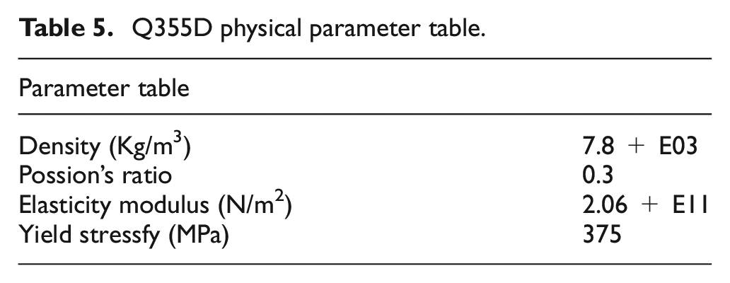
Similarly, by substituting the data in Table 5 and the elastic modulus E = 2.06 $\times {10}^{-13}$ Pa and Poisson’s ratio $v$  = 0.33 into equation (8), the theoretical values of the calibration coefficients A and B can be obtained as $A_t$  = −6.149  $\times {10}^{-13}P{a}^{-1}$ , $B_t=$ −1.409  $\times {10}^{-12}P{a}^{-1}$ respectively.

By comparing the calculated values A and B of the calibration coefficients, it can be found that the errors of the two are −0.37% and 3.83%, respectively, indicating that the strain extraction method is effective and accurate. Table 3 lists the comparison results.

Table 3.

Table of comparison and analysis between calculation value and theoretical value of calibration coefficient A and B.

Calibration coefficient	Theoretical value ( $P{a}^{-1}$ )	Finite element calculated value ( $P{a}^{-1}$ )	Deviation (%)
A	−6.149 $\times {10}^{-13}$	−6.126 $\times {10}^{-13}$	−0.37
B	−1.409 $\times {10}^{-12}$	−1.355 $\times {10}^{-12}$	3.83

Material parameters of U-rib in welding test

Table 4 shows the chemical composition table of the U-ribs selected for the test, and Table 5 shows the physical parameter table. The data comes from steel manufacturers.

Table 4.

Q355D chemical composition table (%).

C	Si	Mn	Ni	P	S	Cr	$\mathrm{C}{\mathrm{u}}^a$
0.43	0.18	0.51	0.025	0.030	0.030	0.020	0.20

Table 5.

Q355D physical parameter table.

Parameter table
Density (Kg/m3)	7.8 + E03
Possion’s ratio	0.3
Elasticity modulus (N/m2)	2.06 + E11
Yield stressfy (MPa)	375

U-rib stiffening plate welding test specimen production and experiment steps

In this experiment, Q355D low-alloy steel was selected, and the length of the member was selected as 1000 mm, before welding, the four corners of the structure are constrained in the same way as the simulated boundaries, The overall structure of U-rib is shown in Figure 15. The welding method is carbon dioxide gas shielded welding. The cross-section size of U-rib was shown in Figure 16, and the material parameters were shown in Tables 4 and 5. Key test steps are as follows:

• (1) First of all, the trapezoid rib with a good angle is welded to the steel plate, and the welding adopts a single pass welding, more than 75% welding penetration, the welding speed is maintained at 10–15 cm/min, the arc voltage is 32 V, and the arc current is 660 A. When welding, it is necessary to wait until one side of the weld is cooled to close to room temperature before welding on the other side, in order to avoid uneven distortion of the component due to temperature increase during welding.

• (2) After the specimen is welded and placed for a week, the part of the outer edge of the stiffened plate is polished first, in order to better contact the strain rosette with the surface of the steel plate.

• (3) Attach the residual stress and strain rosettes to the edge of the steel plate. According to the previous residual stress distribution, the center interval of the strain gauge is 15 mm. The layout diagram of strain rosettes and the arrangement of measuring points are shown in Figures 17 and 18.

• (4) Solder the residual stress and strain rosettes to the JM8813 static strain test system, and then connect the computer to the sensor to measure the strain using software.

• (5) Finally, drill holes in the center position of strain rosettes with a relatively stable magnetic base drill, and use JM8813 static strain test system software on the computer to measure the strain value of residual stress release after drilling, and record the data of the measurement point. The drilling diagram of magnetic drill is shown in Figure 19.

Figure 16.

U Rib section dimension diagram (mm).

Figure 17.

Strain gage rosettes layout diagram.

Figure 18.

U stiffening plate measuring point distribution diagram (unit: mm).

Figure 19.

JD2-16E magnetic seat drilling holes.

Comparison of U-rib test results with simulated values

The specific location of the measuring points is shown in Figure 20. Due to the limited test conditions and test methods, the measuring points near the weld cannot be arranged on the inside of the U-rib, so only the measuring points on the outside of the weld are encrypted, and the settings away from the weld are sparse. The comparison between the obtained test results and the simulated values is shown in Figures 21 and 22.

Figure 20.

JM8813 statical strain indicator.

Figure 21.

The residual stress $\mathrm{\sigma }x$ of the base plate along the path direction is distributed.

Figure 22.

The residual stress σz of the base plate along the path direction is distributed.

As illustrated in Figure 21, the test value at measuring point No. 2 is 9.90 MPa, significantly higher than the simulated value of 0.92 MPa. Measuring points No. 1–7 and No. 19–25 exhibit tensile stress, with test values significantly exceeding the simulated values, yet following the same trend. Measuring points Nos. 8 and 18, located near the weld’s outer side, displayed abrupt changes to compressive stress, mirroring the trend of the simulated values. Measuring points No. 9–17 on the inner side of the U rib showed compressive stress, with increasing values at both ends, consistent with the trend of the simulated values.

Figure 22 shows that the test value at measuring point No. 2 is −7.45 MPa, closely matching the simulated value of −7.37 MPa. For measuring points No. 1–7 and No. 19–25, the compressive stress test values generally exceed the simulated values, with the maximum value observed near the weld, following the same trend. Measuring points Nos. 8 and 18, located near the weld’s outer side, demonstrated abrupt shifts to tensile stress, aligning with the trend of the simulated values. Measuring points No. 9–17 on the U-rib’s inner side exhibited compressive stress, with the maximum value near the weld, consistent with the simulated values’ trend.

Simplified model for equivalent calculation of welding residual stress

The primary forms of stress on steel bridge deck are transverse and longitudinal, with the steel material surfaces near the weld seams exhibiting relatively higher levels of residual stress. Consequently, this article extracts the data on the residual stress distribution on the top surface of the base plate and employs data fitting to derive suitable fitting curves, thereby providing a foundation for practical engineering applications. The fitting curve of residual stress can be utilized as the initial stress condition in finite element models, facilitating convenient calculations using the fitted curve results in engineering software (Tables 6 and 7).

Table 6.

Table of residual stress $f_{\sigma x}(x)$ piecewise function coefficient.

Coefficient A	Value	Coefficient B	Value	Coefficient C	Value	Coefficient D	Value
$A_1$	2.07E+00	$B_1$	8.67E+04	$C_1$	−2.26E+05	$D_1$	−9.85E+02
$A_2$	−4.49E-01	$B_2$	−2.32E+03	$C_2$	4.28E+03	$D_2$	1.18E+01
$A_3$	1.25E-02	$B_3$	2.01E+01	$C_3$	−2.71E+03	$D_3$	−4.76E-02
$A_4$	−7.90E-05	$B_4$	−5.70E-02	$C_4$	5.71E-02	$D_4$	6.34E-05

Table 7.

Table of residual stress $f_{\sigma z}(x)$ piecewise function coefficient.

Coefficient E	Value	Coefficient F	Value	Coefficient G	Value
$E_1$	−6.70E+00	$F_1$	4.03E+05	$G_1$	−2.47E+02
$E_2$	−2.41E-01	$F_2$	−8.46E+03	$G_2$	8.13E-01
$E_3$	7.79E-03	$F_3$	5.90E+01	$G_3$	3.76E-03
$E_4$	−7.28E-05	$F_4$	−1.37E-01	$G_4$	−1.29E-05

This article adopts a piecewise cubic polynomial fitting method for the approximation of the residual stress curve, ensuring that the fitting coefficient R associated with the weld attains a value of 0.9 or above. Since the residual stress distribution is symmetrically distributed about the center of the stiffening plate, it is only necessary to perform curve fitting for one half of the simulated residual stress values. The $\sigma x$ residual stress diagram is simulated using four sections of fitting curves, while the $\sigma z$ residual stress is modeled with three sections of fitting curves (Figures 23 and 24).

$$\begin{array}{l}{f}_{\sigma x}\left(x\right)=\{\begin{array}{c}{A}_1+A_2\times x^1+A_3\times x^2+A_4\times x^3\\ B_1+B_2\times x^1+B_3\times x^2+B_4\times x^3\\ C_1+C_2\times x^1+C_3\times x^2+C_4\times x^3\\ D_1+D_2\times x^1+D_3\times x^2+D_4\times x^3\end{array},\\ \mathrm{when}\{\begin{array}{c}0\le x<\frac{9a}{40}\\ \frac{9a}{40}\le x<\frac{143a}{600}\\ \frac{143a}{600}\le x<\frac{11a}{40}\\ \frac{11a}{40}\le x<\frac{a}{2}\end{array}\end{array}$$

(12)

Figure 23.

The residual stress $\sigma x$ curve of the base plate along the X-axis is fitted.

Figure 24.

The residual stress $\sigma z$ curve of the base plate along the X-axis is fitted.

According to the above method, the curve segment fitting of $\sigma z$ along the base plate x direction is continued to obtain the following segment formula (Figures 25 and 26):

$$\begin{array}{l}{f}_{\sigma x}\left(x\right)=\{\begin{array}{c}{E}_1+E_2\times x^1+E_3\times x^2+E_4\times x^3\\ F_1+F_2\times x^1+F_3\times x^2+F_4\times x^3\\ G_1+G_2\times x^1+G_3\times x^2+G_4\times x^3\end{array},\\ \mathrm{when}\{\begin{array}{c}0\le x<\frac{9a}{40}\\ \frac{9a}{40}\le x<\frac{27a}{100}\\ \frac{27a}{100}\le x<\frac{a}{2}\end{array}\end{array}$$

(13)

Figure 25.

Diagram of segmental function of U-rib stiffener $\sigma x$ fitting curve.

Figure 26.

Diagram of segmental function of U-rib stiffener $\sigma z$ fitting curve.

Conclusion

This article examines residual stress generation in U-ribbed steel bridge deck during welding, focusing on changes in the base material’s residual stress pattern post-welding. A thermo-elasto-plastic finite element analysis model was used to perform numerical simulations of the welding process, extracting and summarizing residual stress changes near the weld seam. To validate the proposed numerical simulation method, the blind hole method was used to measure welding-induced residual stress, and finite element analysis calculated calibration coefficients A and B, demonstrating the method’s effectiveness. Comparing experimental measurements with numerical simulation outcomes confirmed the finite element simulation method’s accuracy and the adopted methodology’s feasibility. Based on these findings, a piecewise linear fitting approach was utilized to develop a simplified model of welding residual stress. The findings of this paper lead to the following conclusions:

• (1) Equivalent residual stresses on both sides of the base plate are symmetrically distributed, with maximum welding residual stresses on both surfaces approaching yield strength. The weld zone and its vicinity, including areas close to the weld on the base plate, exhibit the highest equivalent residual stresses.

• (2) On the top surface of the base plate, transverse residual stress is predominantly compressive, peak transverse residual compressive stress reaches about 0.78 times the material’s yield strength, with a significant stress range in the weld’s heat-affected zone extending about 30 mm, and lower stress values across the base plate. Conversely, the bottom surface’s transverse residual stress is predominantly tensile, with peak stress about 0.75 times the yield strength, directly beneath the weld center.

• (3) Near the weld, the top surface exhibits tensile stress, near the weld peaks about 3mm from the center, which is about 1.17 times the yield strength. This aligns with findings by scholars such as Ji et al. ²¹ Within 30 mm of the weld on both sides, residual tensile stress sharply decreases, peaking at 15 mm from the weld center—approximately the thickness of the rib plate (12 mm)—with the maximum compressive stress being about 0.21 times the yield strength. Similar to the top, with peak tensile stress reaching about 0.77 times the yield strength. Within 25 mm of the weld on both sides, residual tensile stress decreases sharply, transitioning to compressive stress about 8 mm from each side, where the peak compressive stress—about 0.21 times the yield strength—is observed at roughly the rib plate’s thickness (12 mm) from the center.

• (4) Calibration of coefficients A and B through finite element analysis, alongside theoretical comparisons, confirmed the method’s accuracy and validity. Applying calculated values in the blind hole experiment yielded results consistent with simulation trends, demonstrating the method’s effectiveness.

• (5) This article employs a piecewise cubic polynomial fitting method for the residual stress curve, using four segments for the $\sigma x$ stress and three for the $\sigma z$ stress, with a weld-related fitting coefficient R exceeding 0.9. The work in this paper is only applicable to 8 mm thick U-rib and 12 mm thick U-rib bridge panel. The simplified model provides the initial conditions of residual stress for mechanical calculation of U-rib of the same type. It should be noted that the work in this paper is only applicable to the U-rib bridge panel with 8 mm thick U-rib and 12 mm base plate, and the inconsistency of welding methods will affect the accuracy of the simplified curve.