Sage Journals: Discover world-class research

Abstract

During the longitudinal motion of a supercavitating vehicle, the stability control problem is complicated because of the nonlinear planing force on the tail part. The dynamic model of a supercavitating vehicle in longitude plane is nonlinear, simultaneously, the control instructions of a supercavitating vehicle may exceed the physical limits of an actuator. Therefore, designing a longitudinal stability control system for a supercavitating vehicle, not only the treatment of nonlinear planing force, but also the physical constraints of the actuator should be considered. For the longitudinal motion model of supercavitating vehicle, a cascade model is proposed, which decomposes the longitudinal motion of supercavitating vehicle into two subsystems. Sliding mode control based on RBF neural network compensation is adopted in the controller design process, and RBF neural network is exploited to approach the deviation caused by actuator saturation. The proposed control method can effectively compensate the performance degradation caused by control variable saturation, and has strong robustness.

Keywords

Supercavitating vehicle cascade model RBF network sliding mode control

Introduction

In the development process of supercavitating vehicles, mathematical modeling and control technology have always been the most critical parts. When the vehicle is enveloped in a bubble, on the one hand, the resistance encountered by the vehicle sharply decreases, making high-speed navigation possible, and on the other hand, the fluid dynamics and torque balance of the vehicle also change accordingly. These all make the dynamic modeling and control of supercavitating vehicle extremely difficult.

Therefore, studying the mathematical model of supercavitating vehicles and their longitudinal control methods has important theoretical and practical significance.

Because of the viscous resistance of the fluid, the speed of conventional underwater or surface vehicles such as torpedo, AUV, and surface ship are difficult to break the velocity limit. Supercavitating vehicle taking advantage of cavity wrapping can reduce friction resistance of surface fluid remarkably, and its speed can reach 200 m/s with proper propulsion technology. The enveloping of the cavity provides a significant speed advantage, but it also makes the dynamic model of the supercavitating vehicle significantly different from that of other conventional vehicles. A cavitator in front of the supercavitating vehicle and tail rudder at the rear of the vehicle contact with fluid. Interaction between the tail of supercavitating vehicle and cavity wall results in nonlinear planing force. The direction and amplitude of the planing force change nonlinearly with the cavity state and vehicle attitude. The cavity shape depends on the speed of the vehicle, volume of ventilation, volume of air leakage and other factors. Therefore, the dynamics, stability, control, and maneuverability of supercavitating vehicle are different from those of conventional underwater vehicle due to the above reasons. It brings some challenges to research on dynamic modeling and control system design for supercavitating vehicle. In practice, the famous supercavitating vehicle is “Storm” torpedo, it processes straight level flight ability with high speed, however, attitude control in longitudinal plane is required to further study.

In literatures, the research on dynamic modeling of supercavitating vehicle mainly focuses on longitudinal motion^1–5 and six-degree-of-freedom motion,⁶ the state variables selected in longitudinal motion are vertical displacement, longitudinal velocity, pitch angle, and pitch rate of the mass center. The state variables of the six-degree-of-freedom motion model are vertical displacement, longitudinal velocity, pitching angle, pitching rate, angle of attack, and sideslip angle. There are also a few scholars engaging in the research of lateral motion modeling and control,^4,7,8 and dynamic modeling and control of supercavitating vehicle during acceleration stage.^9,10 The longitudinal motion of supercavitating vehicle has been studied extensively, and the models researched are mainly based on those proposed in Dzielski and Kurdila,¹ the model is transformed into an error control model, and then the controller is designed. There are two kinds of longitudinal motion models, one is the model without delay effect, the other is the model with delay effect.

At present, there are mainly linear control methods and nonlinear control methods for longitudinal motion control of supercavitating vehicle. Linear control methods include linear state feedback¹ and LQR.¹¹ A state feedback control method used in Dzielski and Kurdila¹ achieves the initial state stabilization of the supercavitating vehicle. The nonlinear control methods include switching control,^12,13 sliding mode control,^14,15 linear matrix inequality control,^16,17 predictive control,^18–20 LPV control,^21,22 fuzzy control,^23,24 fault-tolerant control,²⁵ adaptive control,^26,27 and so on. In Lin et al.,¹² the longitudinal motion model of supercavitating vehicle is divided into two cases: with and without planing force model according to the critical state of planing force, and a state feedback control is adopted for the case without planing force, a switching control is adopted when the planing force is not zero. The principle of feedback control is simple, and it is easy to realize in practice. However, it is generally effective around the work benchmark. Once the work benchmark changes, feedback parameters need to be regulated again. There are sliding mode control based on upper and lower bounds estimation and globally stable sliding mode control.^14,15 Sliding mode control enables the system to track a time-varying reference signal, but the control variables generally appear chattering phenomenon. A linear matrix inequality approach can be adopted to obtain the asymptotically stable solution of the system, and the gain can make the system asymptotically stable, but the amplitude of the gain is generally large.¹⁶ Literature¹⁹ applies a model prediction method to build a prediction model, and then exploits a linear matrix inequality approach to obtain a feedback gain matrix, the predictive controller can make the longitudinal displacement of the supercavitating vehicle track the time-varying reference signal. Predictive control at each sample point, based on the state of the controlled object and the predictive model, predicts the state of the system in the future period, and solves the optimal control sequence according to a certain performance index (cost function), the first control action of the control sequence enters into the actuator, and the optimization algorithm is executed at the next sampling point. Model predictive control solves optimization problems iteratively at every time step, optimization problems are usually time-consuming, however, the action of the controller has a strong demand for real-time, therefore, the model predictive control is not suitable for the controlled plant which requires high rapidity. A linear parameter-varying (LPV) controller is also synthesized for angle rate tracking in the presence of model uncertainty.²² LPV approximates a nonlinear system to a time-varying linear system, the time-varying parameters are treated into a convex set with several time-invariant parameters as vertices, then Lyapunov function is constructed to deal with the time-varying linear system by using robust control method. LPV ensures the stability in theory. However, LPV approach does not take advantage of the structural characteristics of the system, it simply changes the time-varying parameter into an uncertain parameter set, as a result, sometimes the nonlinear control theory approach has better results with larger areas of attraction and even global attraction. In the literature above, in all the controller design process, the problem of deflection angle constraint of cavitator and tail rudder are seldom considered, most of which are verified by the simulation results that the control variable’s amplitude is in the physically acceptable range, as in literature.²⁶ In Tang et al.,²⁸ a controller is improved by linear active disturbance rejection control (LADRC) method, which provides the additional control component to reduce the rotation angle and rotation speed of the actuator. An anti-saturation compensation method is exploited to overcome the input constraints caused by the physical limitations of the control mechanism. ADRC adopts the method of “Observation + compensation” to deal with the nonlinearity and uncertainty in the control system, the external disturbance/self-disturbance is compensated before it occurs. At the same time, the nonlinear feedback method is used to improve the dynamic performance of the controller. ADRC algorithm is simple, easy to implement, high precision, fast speed, and has strong anti-disturbance ability. Therefore, for the longitudinal motion control of the supercavitating vehicle, it is necessary to ensure that the control system can track a reference signal, and the amplitude of the control variable is within the physical range of the actuator.

To meet the control objective and realize stability of the supercavitating vehicle motion, special attention is paid to longitudinal motion model. In the longitudinal motion model, the control variables only have a direct effect on the changes of vertical velocity and pitch rate, and have an indirect effect on the changes of vertical displacement and pitch angle. Therefore, the theory of cascade system is introduced into the expression of the longitudinal motion model, and the longitudinal motion model is written as a cascade form. The physical constraints of the actuator are considered in the control system, and the amplitude constraints of the control variables are represented by control limitation. The performance loss caused by actuator saturation is compensated by an auxiliary system. The deviation of the control variable with or without saturation is estimated and compensated by RBF neural network. Furthermore, a sliding mode controller is designed to make the system asymptotically stable.

In order to complete the above work, the structure of this paper is organized as follows. In section “Cascade model of longitude motion model,” longitudinal dynamic model and a cascade model of supercavitating vehicle are presented. In section “Control efficiency analysis,” control efficiency is analyzed. In section “Sliding mode anti-saturation control based on RBF neural network compensation,” sliding mode control based on RBF neural network compensation is proposed to solve the problem of actuator saturation. In section “Simulation and analysis,” simulation analysis and verification are conducted. Conclusion remarks are presented in section “Conclusion.”

Cascade model of longitude motion model

Dynamic model

The coordinates of the North East Down and the body are established in accordance with right-hand rule and anticlockwise as positive direction. As shown in Figure 1, the origin of body coordinates coincides with the geometric center of cavitator at the head of the supercavitation vehicle.

Figure 1.

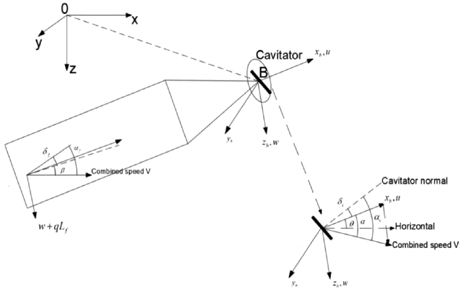
The coordinates diagram.

The depth of the head of the vehicle is $z$ in North East Down frame $O - xyz$ , the horizontal speed along the centerline is $u$ and the vertical speed of the vehicle is recorded as $w$ , the combined speed, or the forward speed, of the vehicle is:

V = \sqrt{u^{2} + w^{2}}

(1)

Since the vertical velocity $w$ is relatively small compared with $u$ , it can be approximated as $V \approx u$ .

Cavitator force

F_{cav} = \frac{1}{2} π ρ {R_{n}}^{2} V^{2} C_{x 0} (1 + σ) a_{c} = C_{l} a_{c}

(2)

α_{c} = \frac{w}{V} + δ_{c}

(3)

$F_{cav}$ is lift provided by the cavitator, $R_{n}$ is radius of the cavitator, $α_{c}$ is attack angle of the cavitator, $δ_{c}$ is deflection angle of the cavitator, $C_{l} = \frac{1}{2} ρ V^{2} π R_{n}^{2} C_{x 0} (1 + σ)$ , $C_{x 0}$ is lift coefficient of zero cavitation number, $σ$ is cavitation number.

Fin lift

In order to generate enough force and torque to balance gravity and control the supercavitating vehicle, the tail fin also provides some hydrodynamic force to produce the control torque. At present, there is no mature research result on the hydrodynamic force of fin of the supercavitating vehicle. When the vehicle is in the state of supercavitating, the fin can be regarded as a wedge-shaped cavitator with special shape in the longitudinal plane, the hydrodynamic analysis of the tail fin is similar to that of the cavitator.

F_{fin} = - n C_{l} α_{f}

(4)

$α_{f}$ is attack angle of fin, the relationship between attack angle and the deflection angle is as follows:

α_{f} = \tan^{- 1} (\frac{w}{V} + \frac{qL}{V}) + δ_{e} \approx \frac{w}{V} + \frac{qL}{V} + δ_{e}

(5)

Defines the anticlockwise direction rotation of the cavitator and tail to be positive for the deflection angle $δ_{e}$ of fin.

Planing force

The planing force is related to the depth of tail immersed in water and the angle between the body and the cavity wall. Its expression is

F_{p} = - V^{2} [1 - {(\frac{R'}{h' + R'})}^{2}] (\frac{1 + h'}{1 + 2 h'}) α

(6)

Its dimension is $m^{2} / s^{2}$ , the planing force here is divided by $m_{p} = ρ π R^{2}$ to standardized formula, $R' = (R_{c} - R) / R$ , $R_{c}$ is the cavity radius, $R$ is the vehicle radius.

w_{th} = \frac{V (R_{c} - R)}{L}

h' = {\begin{matrix} 0 | w | \leq w_{th} \\ \frac{L}{R} | \frac{w}{V} | - \frac{R_{c} - R}{R} | w | > w_{th} \end{matrix}

(7)

α = {\begin{matrix} \frac{w}{V} - \frac{{\overset{\cdot}{R}}_{c}}{V} w > 0 \\ \frac{w}{V} + \frac{{\overset{\cdot}{R}}_{c}}{V} w \leq 0 \end{matrix}

(8)

where $\overset{\cdot}{R_{c}}$ is the change rate of cavity radius.

K_{1} = \frac{L}{R_{n}} {(\frac{1.92}{σ} - 3)}^{- 1} - 1

(9)

K_{2} = {[1 - (1 - \frac{4.5 σ}{1 + σ}) K_{1}^{40 / 17}]}^{1 / 2}

(10)

R_{c} = R_{n} {(0.82 \frac{(1 + σ)}{σ})}^{1 / 2} K_{2}

(11)

{\overset{\cdot}{R}}_{c} = \frac{- \frac{20}{17} {(0.82 \frac{(1 + σ)}{σ})}^{1 / 2} V (1 - \frac{4.5 σ}{1 + σ}) K_{1}^{(23 / 17)}}{K_{2} (\frac{1.92}{σ} - 3)}

(12)

Gravity

Gravity acting on the vehicle is

G = Mg

(13)

Motion equation

According to the small-angle approximation principle, the kinematic model of the supercavitating vehicle is as follows:

\begin{matrix} \overset{\cdot}{z} = w \cos θ - V \sin θ = w - v θ \\ \overset{\cdot}{θ} = q \end{matrix}

(14)

where $z$ is depth, $w$ is vertical speed, $θ$ is pitch angle, $q$ is pitch rate, $v$ is forward speed.

The dynamic model

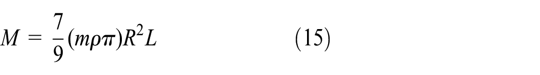
The total length of the vehicle is $L$ , the moment of inertia is $I_{yy}$ , $X_{g}$ is mass center location, $M$ is the mass of the vehicle. $ρ$ is the density of the liquid around the vehicle, $m$ is the density ratio of the vehicle itself and the ambient liquid, and $R$ denotes the radius of aft cylinder.

M = \frac{7}{9} (m ρ π) R^{2} L

(15)

I_{yy} = \frac{11}{60} (m ρ π) R^{4} L + \frac{133}{405} (m ρ π) R^{2} L^{3}

(16)

X_{g} = - \frac{17}{28} L

(17)

The translational dynamics equations described by the North east down $O - xyz$ and the rotational dynamics equations described by the body coordinate system are respectively

\begin{matrix} F_{z} = M (\overset{\cdot}{w} - x_{g} \overset{\cdot}{q} - qV) \\ I_{yy} \overset{\cdot}{q} = M_{y} + M x_{g} (\overset{\cdot}{w} - qV) \end{matrix}

(18)

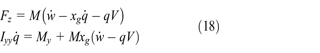
After derivation, it is

\overset{\cdot}{w} = \frac{1}{M - \frac{M^{2} x_{g}^{2}}{I_{yy}}} [(MV - \frac{M^{2} x_{g}^{2} V}{I_{yy}}) q + \frac{M M_{y} x_{g}}{I_{yy}} + F_{z}]

(19)

\begin{matrix} \overset{\cdot}{q} = \frac{M_{y}}{I_{yy}} + \frac{x_{g}}{I_{yy} - {Mx}_{g}^{2}} [(MV - \frac{V M^{2} x_{g}^{2}}{I_{yy}}) q + \frac{M M_{y} x_{g}}{I_{yy}} + F_{z}] \\ - \frac{M x_{g} V}{I_{yy}} q \end{matrix}

(20)

where $F_{z}$ , $M_{y}$ is total force and moment of the vehicle, respectively

F_{z} = F_{cav} + F_{fin} + G + F_{p} m_{p}

(21)

M_{y} = F_{fin} L - G x_{g} + F_{p} m_{p} L

(22)

$G$ is gravity of the vehicle, $G = Mg$ . Combine (19), (20), (14), we obtain

[\begin{matrix} \overset{\cdot}{z} \\ \overset{\cdot}{w} \\ \overset{\cdot}{θ} \\ \overset{\cdot}{q} \end{matrix}] = [\begin{matrix} 0 & 1 & - V & 0 \\ 0 & a_{22} & 0 & a_{24} \\ 0 & 0 & 0 & 1 \\ 0 & a_{42} & 0 & a_{44} \end{matrix}] [\begin{matrix} z \\ w \\ θ \\ q \end{matrix}] + [\begin{matrix} 0 \\ b_{2} \\ 0 \\ b_{2} \end{matrix}] δ_{c} + [\begin{matrix} 0 \\ c_{2} \\ 0 \\ 0 \end{matrix}] + [\begin{matrix} 0 \\ d_{2} \\ 0 \\ d_{4} \end{matrix}] F_{p}

(23)

It could be written as follows:

\overset{\cdot}{x} = Ax + Bu + C + D F_{p}

(24)

where $x$ is state variable, $x = {[\begin{matrix} z & w & θ & q \end{matrix}]}^{T}$ , $F_{p}$ is planing force.

Cascade model of longitude motion

Consider a system $\overset{\cdot}{x} = f (t, x)$ that can be written as

{\begin{matrix} {\overset{\cdot}{x}}_{1} = f_{1} (t, x_{1}) + g (t, x_{1}, x_{2}) x_{2} \\ {\overset{\cdot}{x}}_{2} = f_{2} (t, x_{2}) \end{matrix}

(25)

where $x_{1} \in R^{n}, x_{2} \in R^{m}, f_{1} (t, x_{1})$ is continuously differentiable in $(t, x_{1})$ . $f_{2} (t, x_{2})$ and $g (t, x_{1}, x_{2})$ are continuous in their arguments, and locally Lipschitz in $x_{2}$ and $(x_{1}, x_{2})$ respectively.

Notice that if $x_{2} = 0$ , (25) reduces to

{\overset{\cdot}{x}}_{1} = f_{1} (t, x_{1})

(26)

Therefore, it can be viewed as the system

\sum_{1} : {\dot{x}}_{1} = f_{1} (t, x_{1})

(27)

that is perturbed by the output of the system

\sum_{2} : {\dot{x}}_{2} = f_{2} (t, x_{2})

(28)

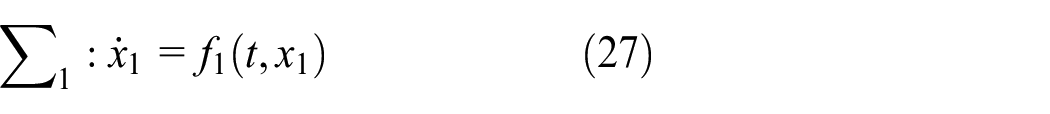
Even if systems $\sum_{1}$ and $\sum_{2}$ are both asymptotically stable, the cascade system in equation (25) is not always asymptotically stable (Lefeber et al.)²⁹.

According to the definition of cascade system, the longitudinal motion model of supercavitating vehicle can be written in cascade form. The dynamic model of the supercavitating vehicle is rewritten as the subsystem form as follow

[\begin{matrix} \overset{\cdot}{z} \\ \overset{\cdot}{θ} \end{matrix}] = A_{1} [\begin{matrix} z \\ θ \end{matrix}] + B_{1} [\begin{matrix} w \\ q \end{matrix}] \sum_{1}

(29)

Subsystem 1 is used for position control, where the state variable $(w, q)$ can be regarded as the interference of subsystem 1, where $A_{1} = [\begin{matrix} 0 & - V \\ 0 & 0 \end{matrix}]$ , $B_{1} = [\begin{matrix} 1 & 0 \\ 0 & 1 \end{matrix}]$ .

\begin{matrix} [\begin{matrix} \overset{\cdot}{w} \\ \overset{\cdot}{q} \end{matrix}] = A_{2 N} [\begin{matrix} w \\ q \end{matrix}] + B_{2 N} [\begin{matrix} δ_{c} \\ δ_{f} \end{matrix}] + G + D_{ζ} F_{p} \sum_{2} \end{matrix}

(30)

In subsystem 2, the control variable makes system 2 stable, and then makes subsystem 1 stable.

A_{2 N} = [\begin{matrix} a_{11} & a_{12} \\ a_{21} & a_{22} \end{matrix}], B_{2 N} = [\begin{matrix} b_{11} & b_{12} \\ b_{21} & b_{22} \end{matrix}], G = [\begin{matrix} g_{11} \\ g_{21} \end{matrix}], D_{ζ} = [\begin{matrix} d_{11} \\ d_{21} \end{matrix}] .

where

\begin{matrix} a_{11} = \frac{CVn (8398 L^{2} - 10692 R^{2})}{1891 m L^{3} + 8316 mL R^{2}}, \\ a_{12} = \frac{V}{1891 L^{2} + 8316 R^{2}} [\frac{7}{9} - \frac{Cn (46692 L^{2} + 10692 R^{2})}{m}] \\ a_{21} = - \frac{17820 CVn}{(1891 L^{2} + 8316 R^{2}) m}, \\ a_{22} = \frac{LV}{(1891 L^{2} + 8316 R^{2})} (\frac{17}{36} - \frac{17820 Cn}{m}) \\ b_{11} = \frac{36 C V^{2} n (233 L^{2} - 297 R^{2})}{1891 m L^{3} + 8316 mL R^{2}}, \\ b_{12} = \frac{36 C V^{2} (532 L^{2} + 297 R^{2})}{1891 m L^{3} + 8316 mL R^{2}}, \\ b_{21} = \frac{- 17820 C V^{2} n}{1891 m L^{2} + 8316 m R^{2}}, \\ b_{22} = \frac{- 27540 C V^{2}}{1891 m L^{2} + 8316 m R^{2}}, \\ c_{11} = g \\ c_{21} = 0 \\ d_{11} = \frac{36 (297 R^{2} - 233 L^{2})}{1891 m L^{2} + 8316 m R^{2}}, \\ d_{21} = \frac{17820 L}{1891 m L^{2} + 8316 m R^{2}} \end{matrix}

Control efficiency analysis

From the dynamic model of supercavitating vehicle, it can be seen that the control variables are mainly cavitator and fins. The efficiency of the control variables is analyzed, and the influence of the different deflections of the cavitator and the stern rudder on the attitude of the vehicle is analyzed under open-loop condition. The control variable of the longitudinal motion is determined by setting a fixed value of the cavitator deflection to judge the effect of the cavitator on four longitudinal states of the vehicle. Set the cavitator deflection angle as −0.001 rad when the state response is shown in Figure 2.

Figure 2.

Open-loop response with $δ_{c} = - 0.001 rad$ .

When the rudder deflection angle is 0.01 rad, the cavitator deflection angle is −0.0009 rad (Figure 3). The simulation results are

Figure 3.

Open-loop response with $δ_{c} = - 0.0009 rad$ and $δ_{e} = 0.01 rad$ .

Both deflection of cavitator and tail rudder can change the attitude of the supercavitating vehicle. Therefore, the deflection angle of the cavitator has been used as a control variable in many literatures. It can also be seen from the figure above, the proper deflection of the cavitator can adjust the attitude of the vehicle, and the attitude of the vehicle is sensitive to the deflection angle of cavitator.

Sliding mode anti-saturation control based on RBF neural network compensation

System composition

In practical, because of the limit of the actuator deflection angle, the amplitude of the control variable is usually restricted, large control amplitude is difficult to achieve. It is meaningful to design effective control algorithm under the condition of control input constraint, which is the control input saturation problem. For the anti-saturation problem, the general method is to conduct a control method based on control input saturation by constructing an auxiliary system and adopting the method of amplification of input saturation dynamic error. Many methods can be exploited in the controller design, such as sliding mode control. The control system composition block diagram is shown in Figure 4.

Figure 4.

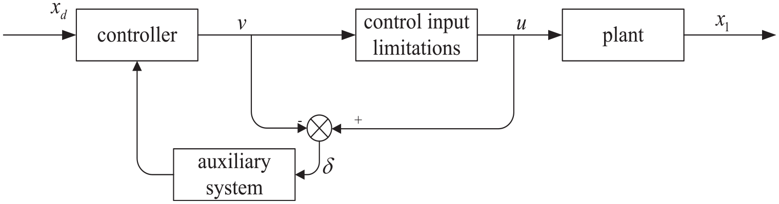
The block diagram of system.

Through designing a stable adaptive auxiliary system, and the estimation of the deviation of $v$ and $u$ can achieve control saturation compensation. In this paper, the universal approximation ability of RBF neural network is adopted to approximate $δ$ , and sliding mode control method is used to design the controller. The diagram of the closed-loop control system is shown in Figure 5.

Figure 5.

The block diagram of system with RBF neural network.

It can be seen from the graph that when the system appears actuator saturation, the output of sliding mode controller is $v$ , $v$ passes through RBF neural network, and the approximation of the difference between $v$ and $u$ is estimated by RBF, and the approximation is added to the control law of the sliding mode controller, so that the amplitude of the control law is not larger than the limit of the actuator, and the saturation of the actuator can be avoided.

RBF neural network structure

RBF neural network model is a kind of neural network structure proposed by Moody and Darken in 1988. It belongs to the type of forward neural network and can approach any continuous function with arbitrary precision, the neural network is an activation function based on radial basis function. The RBF neural network is a three-layer forward network. The first layer is the input layer composed of the source nodes, and the second layer is the hidden layer, the number of hidden units depends on the requirement. The transformation function of hidden units is a non-negative nonlinear function called RBF (radial basis function). The third layer is the output layer, which is a linear combination of the output of hidden layer neurons, the topology of RBF neural network is shown in Figure 6.

h_{j} (t) = \exp (- \frac{{‖ x (t) - c_{j} (t) ‖}^{2}}{2 b_{j}^{2}}), j = 1, \dots, n

(31)

\hat{f} (x) = {\hat{W}}^{T} h (x) + ε

where $x$ is the input of the network, $i$ is the $i^{th}$ input of the input layer of the network, $j$ is the $j^{th}$ input of the hidden layer of the network, $h = {[h_{j}]}^{T}$ is the output of the Gauss function, $W^{*}$ is the ideal weight of the network, $ε$ is the approximation error of $δ$ of the ideal neural network, $ε \leq ε_{max}$ , $\hat{δ}$ is network output. According to Figure 5, the input of the network is $x = v$ , and the output of the network is $\hat{δ} = {\hat{W}}^{T} h$ , $\hat{W}$ is the estimated weight of the neural network. If the estimated error of the weight is $\tilde{W} = \hat{W} - W^{*}$ , then the estimated error of $δ$ is $δ - \hat{δ} = - {\tilde{W}}^{T} h + ε$ .

Figure 6.

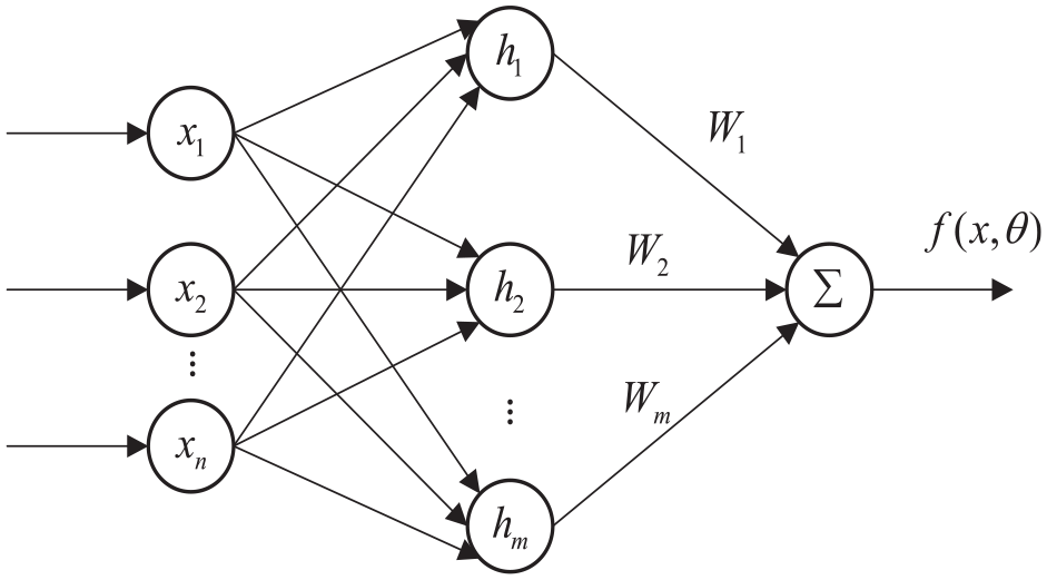
RBF neural network topology.

Sliding mode controller design

Control target is $x \to x_{d}$ , $x_{d}$ is command signal, error between command signal and actual signal is $e = x - x_{d}$ , then $\overset{\cdot}{e} = \overset{\cdot}{x} - {\overset{\cdot}{x}}_{d}$ . Sliding mode function is

s = c_{1} e_{1} + c_{2} e_{2} + {\overset{\cdot}{e}}_{1} + {\overset{\cdot}{e}}_{2}

(32)

where $c_{1} > 0$ , $c_{2} > 0$ , then

\begin{matrix} \overset{\cdot}{s} = c_{1} {\overset{\cdot}{e}}_{1} + c_{2} {\overset{\cdot}{e}}_{2} + {\overset{\cdot\cdot}{e}}_{1} + {\overset{\cdot\cdot}{e}}_{2} \\ = c_{1} {\overset{\cdot}{e}}_{1} + c_{2} {\overset{\cdot}{e}}_{2} + {\overset{\cdot\cdot}{x}}_{1} - {\overset{\cdot\cdot}{x}}_{1 d} + {\overset{\cdot\cdot}{x}}_{2} - {\overset{\cdot\cdot}{x}}_{2 d} \\ = c_{1} {\overset{\cdot}{e}}_{1} + c_{2} {\overset{\cdot}{e}}_{2} \\ + [\begin{matrix} - V x_{2} + (A_{011} + A_{021}) x_{3} + (A_{012} + A_{022}) x_{4} \\ + (B_{012} + B_{022}) u + C_{011} + C_{021} + (D_{011} + D_{021}) F_{p} \end{matrix}] \\ - {\overset{\cdot\cdot}{x}}_{1 d} - {\overset{\cdot\cdot}{x}}_{2 d} \end{matrix}

(33)

Lyapunov function is

V = \frac{1}{2} s^{2} + \frac{1}{2} γ {\tilde{W}}^{T} \tilde{W}

(34)

where $γ > 0$ , it is adaptive law.

Theorem 1. For the longitudinal motion model of supercavitating vehicle, the necessary and sufficient condition for its asymptotic stability is that the control variable is

\begin{matrix} u = \frac{1}{(B_{012} + B_{022})} \\ [\begin{matrix} - c_{1} {\overset{\cdot}{e}}_{1} - c_{2} {\overset{\cdot}{e}}_{2} + V x_{2} - (A_{011} + A_{021}) x_{3} - (A_{012} + A_{022}) x_{4} \\ + {\overset{\cdot\cdot}{x}}_{1 d} + {\overset{\cdot\cdot}{x}}_{2 d} - η sgn (s) \end{matrix}] - \hat{δ} \end{matrix}

(35)

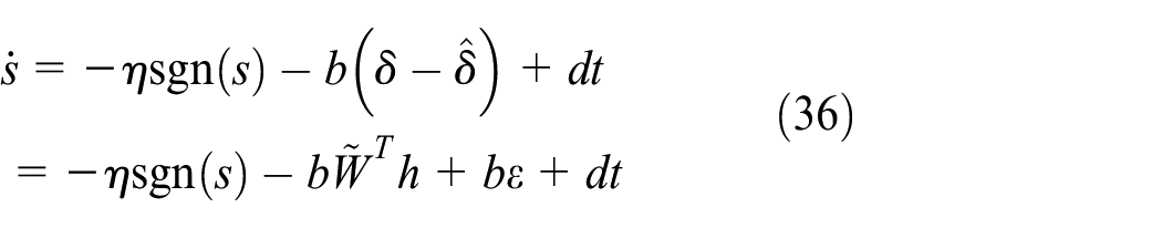
Proof. From a sliding mode switching law (33), equation (36) is obtained

\begin{matrix} \overset{\cdot}{s} = - η sgn (s) - b (δ - \hat{δ}) + dt \\ = - η sgn (s) - b {\tilde{W}}^{T} h + b ε + dt \end{matrix}

(36)

Take it into equation (34), then

\overset{\cdot}{V} = s \overset{\cdot}{s} + γ {\tilde{W}}^{T} \overset{\cdot}{\tilde{W}} = - η | s | + sdt + sb ε + {\tilde{W}}^{T} (- sbh + γ \overset{\cdot}{\hat{W}})

(37)

Take the law of adaptation as

\hat{W} = \frac{1}{γ} sbh

(38)

then

\overset{\cdot}{V} = - η | s | + s (dt + b ε) \leq 0

(39)

end.

Simulation and analysis

Simulation process

According to Figure 5, a closed-loop system is built, which consists of three closed-loops, the first loop is RBF neural network, the second loop is controller limiter to calculate the difference before and after limiter, and the outermost loop is output feedback of the system. Before the simulation, the initial conditions, the reference signal and the initial weights of the RBF neural network are set. At the beginning of the simulation, $x_{d}$ passes through a sliding mode controller, sliding mode controller outputs $v$ . A branch of $v$ is used as the RBF input, and calculates output $\hat{δ}$ through (31). At the same time, the other branch of $v$ , passes through the control input limitations, if $v$ exceeds the amplitude limit, it outputs $\pm 1.4 rad$ . If the amplitude value is not reached, then the original value output to the controlled plant (supercavitating vehicle). The attitude of the controlled plant outputs and feedbacks to the sliding mode controller with RBF neural network. At this time, $\hat{δ}$ has been calculated, and $\hat{δ}$ is the compensation value when the actuator is saturated. The next simulation step, in accordance with the above process, $\hat{δ}$ and $x_{d}$ produce system output, such a cycle, until the system is stable, the simulation is stop.

In the whole simulation process, RBF neural network calculates and updates the weight value by accepting the external input signal, which is related to whether the actuator of the system is saturated or not, and estimates the difference of actuator saturation and inputs to sliding mode controller for compensation.

The RBF neural network is constructed with a typical 1-5-1 structure. In the training process, because the sliding mode controller has been designed, it is equivalent to training the network through the data generated by each simulation step of the system, the longer the time is, the more the network is trained, the better effect of the convergence.

The output of RBF is the input of sliding mode controller, refer to formula (35), and the output $v$ of sliding mode controller is the input of RBF, as shown in Figure 5. In this way, the integration of sliding mode controller and RBF neural network is realized.

Simulation results and analysis

When the ideal reference signal is step signal, the amplitude of the deflection angle of cavitator is $\pm 1.4 rad$ , which indicates the ability of the control system to compensate for the limited control input, and the initial condition of the system is [0, 0, 0, 0], the structure of RBF network is 1-5-1, the input of network is $x = v$ , parameter of Gauss function is designed according to actual range of input of network, $c_{i} = 6 \times [\begin{matrix} - 1.0 & - 0.5 & 0 & 0.5 & 1.0 \end{matrix}]$ , $b_{j} = 5$ , the initial value of network weight is 0, $c_{1} = c_{2} = 50$ in the sliding mode control law, $γ = 10$ in the adaptive law, the saturation function is exploited to take place of the switching function, and the boundary-layer thickness is $Δ = 0.001$ . Physical parameters of vehicle refer to Dzielski and Kurdila,¹ as shown in Table 1.

Table 1.

Model parameters of supercavitating vehicle.

Symbol	Name	Value (unit)
$ρ_{v}$	Vehicle density	02000 ( $kg / m^{3}$ )
$R$	Vehicle radius	0.0508 ( $m$ )
$L$	Vehicle length	1.8 ( $m$ )
$V$	Vehicle forward speed	75 ( $m / s$ )
$m$	Density ratio ( $ρ_{v} / ρ$ )	2
$g$	Gravitational acceleration	9.81 ( $m / s^{2}$ )
$σ$	Cavitation number	0.02, 0.03
$n$	Rudder effectiveness coefficient	0.5
$C_{x 0}$	Lift coefficient	0.82
$R_{n}$	Radius of the cavitator	0.0191 ( $m$ )

Figure 7 shows the tracking effect of the control system to the reference displacement signal. For the step reference signal with an amplitude of 1, the output can track the reference signal, and the error is in the acceptable range.

Figure 7.

Step response curve.

Figure 8 is the estimation of deviation by RBF network as control amplitude is limited where the red line is the actual error caused by the saturation of the actuator. It can be seen that there is a big error in the estimation of derivation of control limit at the beginning, which then gradually convergence. After 0.5 s, it can achieve unbiased estimation.

Figure 8.

Estimation of deviation by RBF network and control input.

Figure 9 shows the tracking effect of the control system to the reference displacement signal. For the sinusoidal reference instruction signal with an amplitude of 5 m, the output can track the reference instruction signal, and the error is in acceptable range.

Figure 9.

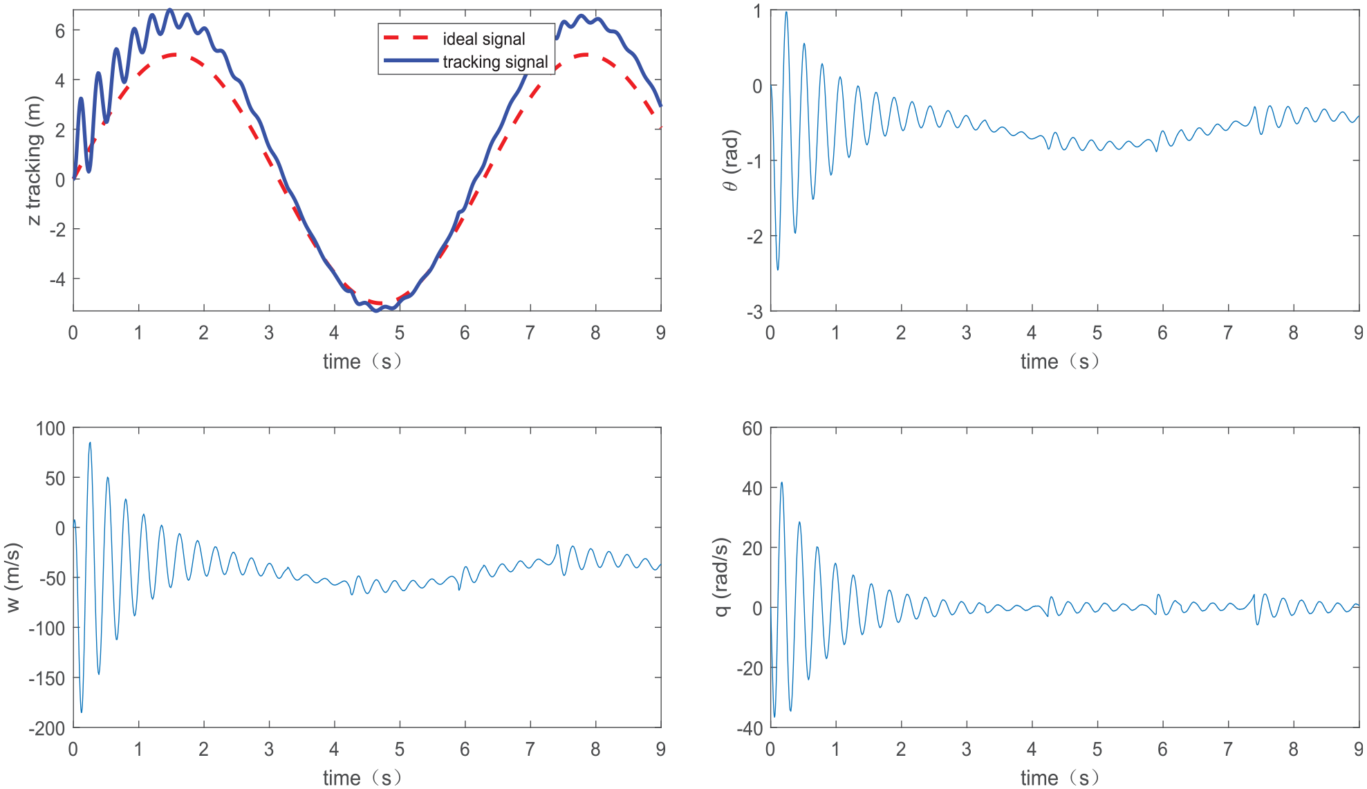
Tracking result of sinusoidal reference instruction signal.

Figure 10 shows the estimation result of the control amplitude limit deviation by RBF network. The red line shows the actual error caused by actuator saturation, then gradually convergence. If the time is long enough, unbiased estimation can be achieved. For the control input response, the red line is control input when there is no amplitude limit, while the blue line is the control input with control limit. It can be seen that when the control input exceeds the amplitude limit, the control amplitude maintains the maximum value, in this amplitude range, the control variables exceed the limit of maximum amplitude at 4, 6, and 7.5 s.

Figure 10.

Estimation result of the control amplitude limit deviation and control input.

Conclusion

In this paper, cascade model of a supercavitating vehicle is presented. Considering the control saturation phenomena in the control system. A RBF neural network is exploited to estimate the controller error between actuator and the control command. Based on the cascade system and RBF neural network, a sliding mode control is proposed to control the system and the Lyapunov function is established to prove the stability of the system. From the simulation results, when the control command exceeds the actuator limit, the RBF neural network has nonzero output and compensates error induced by the physical limitation. The system can track step reference signal and sine signal with permission accuracy.

The main advantage of this method in this paper is that it can compensate the saturation of the actuator in a limited range when the actuator is saturated, so that the sliding mode controller can guarantee the system not to be wind-up when it generates the control law, and ensures the performance of the control system. The disadvantage of this method is that it cannot guarantee global optimization, that is, the parameters of the controller need to be adjusted when the dynamic model of the supercavitating vehicle changes. At the same time, the anti-saturation compensation of the longitudinal motion of the supercavitating vehicle is only studied in this paper. The research of six-freedom maneuver control is the direction of future research.

Footnotes

Handling Editor: Sharmili Pandian

Declaration of conflicting interests

The author(s) declared no potential conflicts of interest with respect to the research, authorship, and/or publication of this article.

Funding

The author(s) disclosed receipt of the following financial support for the research, authorship, and/or publication of this article: This work was supported in part by the National Nature Science Foundation of China under Grant (51879060) and Nature Science Foundation Heilongjiang province (LH2021E044) and (LH2020E069).

ORCID iD

Shangze Chen

References

Dzielski

Kurdila

A benchmark control problem for supercavitating vehicles and an initial investigation of solutions. J Vib Control 2003; 9: 791–804.

Vanek

Bokor

Balas

. Theoretical aspects of highspeed supercavitation vehicle control. In: Proceedings of the American control conference, Minneapolis, MN, USA, 14–16 June 2006, p.6. New York: IEEE.

Nguyen

Balachandran

. Supercavitating vehicles with noncylindrical, nonsymmetric cavities: dynamics and instabilities. J Comput Nonlinear Dyn 2011; 6: 041001.

Kim

. Integrated dynamics modeling for supercavitating vehicle systems. Int J Nav Archit Ocean Eng 2015; 7: 346–363.

Baek

Cho

Han

. Practical time-delay control with adaptive gains for trajectory tracking of robot manipulators. IEEE Trans Ind Electron 2018; 65: 5682–5692.

Kirschner

Kring

Stokes

, et al. Control strategies for supercavitating vehicles. J Vib Control 2002; 8: 219–242.

Luo

Dang

, et al. Nonlinear time delay kinematic model of underwater maneuverable supercavitating vehicles. In: 2010 second international conference on intelligent human-machine systems and cybernetics, Nanjing, China, 26–28 August 2010, pp.84–88. New York: IEEE.

Huang

Luo

Dang

, et al. Spatial kinetics model of supercavitating vehicles reflecting conic-like oscillation. Math Prob Eng 2017; 2017: 1–12.

Wang

J-H

K-P

Wei

Y-J

, et al. Motion stability and control of supercavitating vehicle with variable cavitation number. J Harbin Inst Technol 2011; 18: 19–23.

10.

Chen

Cao

Wang

, et al. Acceleration stage control design for supercavitating vehicle. J Harbin Inst Technol 2016; 48: 147–153. (in Chinese)

11.

Zhang

Wei

Han

, et al. Design and comparison of LQR and a novel robust backstepping controller for supercavitating vehicles. Trans Inst Meas Control 2017; 39: 149–162.

12.

Lin

Balachandran

Abed

. Dynamics and control of supercavitating vehicle. J Dyn Syst Meas Control 2008; 130: 021003.

13.

Shao

Mesbahi

Balas

. Planing, switching, and supercavitating flight control. In: AIAA guidance, navigation, and control conference and exhibit, Austin, TX, USA, 11–14 August 2003.

14.

Zhao

. Sliding mode controller design for supercavitating vehicles. Ocean Eng 2019; 184: 173–183.

15.

Wei

, et al. Design of gain adaptive global sliding mode controller for supercavitating vehicle. J Vib Shock 2011; 30: 34–37+46.

16.

Zhang

Han

Bai

, et al. H∞ controller design using LMIs for high-speed underwater vehicles in presence of uncertainties and disturbances. Ocean Eng 2015; 104: 359–369.

17.

Zhang

Wei

, et al. Finite-time robust H∞ control for high-speed underwater vehicles subject to parametric uncertainties and disturbances. J Mar Sci Technol 2017; 22: 201–218.

18.

Han

Guan

. Predictive control of a supercavitating vehicle based on time-delay characteristics. IEEE Access 2021; 9: 13499–13512.

19.

Han

Guo

. Robust predictive control of a supercavitating vehicle based on time-delay characteristics and parameter uncertainty. Ocean Eng 2021; 237: 109627.

20.

Hui

Zhang

Wang

. Model predictive control design for supercavitating vehicles with control efforts restriction. 2011 international conference on electric information and control engineering, Wuhan, China, 15–17 April 2011, pp.5098–5101. New York: IEEE.

21.

Mao

Wang

. Nonlinear control design for a supercavitating vehicle. IEEE Trans Control Syst Technol 2009; 17: 816–832.

22.

Vanek

Balas

Arndt

REA

. Linear, parameter-varying control of a supercavitating vehicle. Control Eng Pract 2010; 18: 1003–1012.

23.

Mardani

Danesh

Karimi

. Fuzzy/neuro-fuzzy depth and pitch regulating control of a supercavitating vehicle. In: 2011 19th Iranian conference on electrical engineering, Tehran, Iran, 17–19 May 2011.

24.

Zhang

Wang

Liu

. Fast position tracking control of PMSM under high frequency and variable load. Int J Comput Appl Technol 2021; 67: 214–223.

25.

Bai

Biggs

Zhang

, et al. Adaptive fault-tolerant control for longitudinal motion of supercavitating vehicles. Eur J Control 2021; 57: 263–272.

26.

Mao

Wang

. Adaptive control design for a supercavitating vehicle model based on fin force parameter estimation. J Vib Control 2015; 21: 1220–1233.

27.

Yang

Mingyong

Xiaojian

, et al. Global approximation based adaptive RBF neural network control for supercavitating vehicles. J Syst Eng Electron 2018; 29: 797–804.

28.

Tang

Zhao

Wang

, et al. Improved genetic algorithm based optimization design of active disturbance rejection controller. Shangdong Sci 2016; 29: 1–8.

29.

Lefeber

Pettersen

Nijmeijer

. Tracking control of an underactuated ship[J]. IEEE transactions on control systems technology: A publication of the IEEE Control Systems Society, 2003; 11(1): 52–61.

Anti-windup design for supercavitating vehicle based on sliding mode control combined with RBF network

Abstract

Keywords

Introduction

Cascade model of longitude motion model

Dynamic model

Cavitator force

Fin lift

Planing force

Gravity

Motion equation

The dynamic model

Cascade model of longitude motion

Control efficiency analysis

Sliding mode anti-saturation control based on RBF neural network compensation

System composition

RBF neural network structure

Sliding mode controller design

Simulation and analysis

Simulation process

Simulation results and analysis

Conclusion

Footnotes

Declaration of conflicting interests

Funding

ORCID iD

References