Sage Journals: Discover world-class research

Abstract

The performance of model predictive control strategies for hybrid electric vehicles (HEVs) highly depends on the accuracy of future speed predictions. This paper proposes improved prediction models for deterministic model predictive control (DMPC) and stochastic model predictive control (SMPC), respectively. For DMPC, the neural network-based predictor is first introduced and taken as the benchmark predictor. A novel deterministic predictor considering historical prediction errors is proposed, which relies on the assumption that the offset between the prediction and measurement at current instant is a good estimate of the offset in the short future. Based on the proposed deterministic predictor, a stochastic predictor that considers the distribution law of historical data at different locations is further proposed for SMPC. Simulation results show that the controller using the proposed deterministic prediction model improves fuel economy by 2.89%, and the controller using the proposed stochastic prediction model improves fuel economy by 4.5% compared with the benchmark.

Keywords

Energy management dynamic programming model predictive control stochastic prediction model hybrid electric vehicle

Introduction

In the next 50 years, the world’s population will grow from 6 to 10 billion, and the number of cars will increase from 700 million to 2.5 billion.¹ If all these vehicles continue to be driven by internal combustion engines, the oil resources consumed, the amount of exhaust gas emitted, and the environmental pollution problems that follow will be unimaginable.² These factors force us to rapidly develop alternative energy-driven vehicles. It is against this background that new energy vehicles have come into people’s attention. Broadly speaking, new energy vehicles include electric vehicles (EVs), hybrid electric vehicles (HEVs), and fuel cell vehicles (FCEVs).^3,4 However, there are still unbroken technical bottlenecks at this stage, whether it is conventional batteries used in electric vehicles or fuel cells in fuel cell vehicles. Therefore, as a transitional model, HEVs will occupy more and more market shares and develop toward diversification and high performance. On the other hand, the performance of HEVs also depends on the control strategy. Therefore, an effective energy management strategy is crucial to exploit the energy saving potential of HEVs.

A large amount of research has been conducted on energy management strategies (EMS).^5–7 The rule-based control strategy is the easiest and most widely used control strategy. As the design of this strategy is based entirely on expert experience, the best performance usually can only be achieved under specific road conditions. The performance may drop significantly when the road condition changes.⁸ The dynamic programming (DP) algorithm based on Bellman’s optimality principle is widely used in the energy management of HEVs because it can obtain the theoretical global optimal solution.⁹ However, the global optimal solution can be obtained by DP only when the complete road conditions are known, which is impossible in practical applications. And the computational burden of DP increases exponentially with the increase of number of variables, which cannot be deployed in real-time applications. Despite these shortcomings, DP still has great practical value, it can be used as a benchmark to revise the parameters of other control strategies, or used to compare with other control strategies to verify the gap between other control strategies and optimal strategy.^10,11 Another important class of control strategies is based on convex optimization, which has great value in real-time applications due to its short computational method. In DP, the model of the problem can be nonlinear, non-convex, and mixed integer. However, the convex optimization problem has strict requirements on the description form of the problem, and any problem must be approximated as a convex optimization problem, so only the approximate optimal problem can be obtained.^12–14 Besides convex optimization, another commonly used real-time control strategy is Equivalent Consumption Minimization Strategy (ECMS).^15–17 The performance of ECMS has a lot to do with the choice of equivalent factor. A suitable equivalent factor can make the performance of the control strategy approach that of DP.¹⁸ However, in practical applications, the selection of equivalent factors is still a difficult problem,¹⁹ the table-based strategies are still the most widely used. In addition, ECMS does not take into account future road conditions, which also limits its performance.

Another type that is considered to have great application potential in the energy management of new energy vehicles is model predictive control (MPC).^7,20,21 MPC can achieve a balance between performance and computational burden. Compared with EMCS, its performance is significantly improved, and the computational burden is much smaller than that of DP. Therefore, it is considered to be the most valuable control strategy in actual deployment.^22–24 So far, MPC has been widely studied by enterprises and scholars, and a series of research results have been achieved. It has been widely used in the energy management of many different types of new energy vehicles, such as FCVs, HEVs, and EVs.²⁵ Depending on whether the uncertainty of future driving information is taken into account, MPC can be further divided into two categories: deterministic MPC and stochastic MPC. In deterministic MPC, a deterministic predictor for predicting the exact trajectory of future vehicle speed or demand torque is required, which is usually difficult and the prediction performance can only be guaranteed in a short prediction horizon. After the predicted trajectory is obtained through the predictor, some optimization algorithms, such as DP algorithm, quadratic programming (QP) algorithm, or nonlinear programming algorithms, are used to solve the optimal control strategy corresponding to the predicted trajectory. Then the first control command of the control strategy is taken as the optimal control action at the current moment, and this process is repeated in each MPC update cycle.²⁶

In stochastic MPC (SMPC), the purpose of the predictor is not to predict the exact trajectory of future driving information, but the probability distribution of vehicle speed or demand torque. The goal of the SMPC controller is to minimize the expectation of the cumulative coast function in the prediction horizon, which is usually solved by stochastic dynamic programming (SDP). The computational burden of SDP also grows exponentially with the number of variables, so the optimal control strategy is usually saved in the form of a table. In practical deployment, online computation is replaced by looking up the table.²⁷ The performance of DMPC and SMPC both depends on the design of the controller and the accuracy of the prediction model.²⁸ If the accuracy of the prediction model cannot be guaranteed, even the optimal controller may obtain a poor control action, so a predictor that accurately reflects the changes of future driving information is the basis of a high-performance MPC. A variety of speed predictive models already exist for deterministic MPC, including exponential decay models,²⁹ autoregressive moving average (ARMA) method,³⁰ neural network-based models, Markov models, etc.³¹ Some methods of using the information during driving to correct the prediction model in real time have also been proposed, such as using the prediction error of the previous instant to correct the prediction error of the future.³² Some paper proposes a novel robust coordinated decision-making technique via robust multiagent reinforcement learning to coordinate the longitudinal and lateral driving decisions of an automated vehicle while ensuring policy robustness against observational uncertain-ties.³³ A strategy incorporates active disturbance rejection current compensation (ADRCC) to achieve a speed difference of zero at two ends of the half-shaft as the tracking control target, and compensating current is superimposed on the original given current of the motor controller to investigate the electromechanical coupling dynamics and vibration characteristics of the system under impact conditions.³⁴ And an article aims to identify robust objective evaluation criteria for the nonlinear combined longitudinal and lateral dynamics of a vehicle.³⁵ For stochastic MPC, most of the existing prediction models are based on Markov chains (MC). The prediction accuracy of MC-based predictors is completely dependent on historical data and is usually only valid for specific road conditions. And these prediction models are based on the assumption that the transfer process of vehicle speed conforms to the Markov property, but this is not necessarily true in the actual driving process. Except for Markov chain-based predictors, there are few studies on other stochastic prediction models, and most of the studies on SMPC focus on the design of control strategies. However, the performance of SMPC is limited by the predictors, and more precise prediction models can further mine the potential of the controller.

The further improve the performance of MPC, this paper proposes a novel deterministic speed predictor for DMCP and a stochastic speed predictor for SMPC. The main contributions are as follows: (1) An improved deterministic predictor is proposed, which takes into account the error of historical prediction; (2) An improved stochastic predictor combining the deterministic predictor and the stochastic term is proposed, which takes into account the distributional randomness of historical data; (3) A comprehensive analysis is performed through simulations, the application potential of proposed predictors is verified.

The rest of this paper is structured as follows: section “Problem formulation” introduces the mathematical model of HEV and driving scenario. sections “Deterministic prediction and DMPC” and “Stochastic prediction and SMPC” reports the DMCP and SMPC strategies, respectively. Then section “Simulations and discussions” presents the simulation results and analysis. Section “Conclusion” is the main conclusions of this paper.

Problem formulation

In this section, the driving scenario is introduced and the mathematical model of the Parallel Hybrid Electric Vehicles (PHEVs) is established. Then, the optimal control problem is described and formulated in the MPC form.

Driving scenario

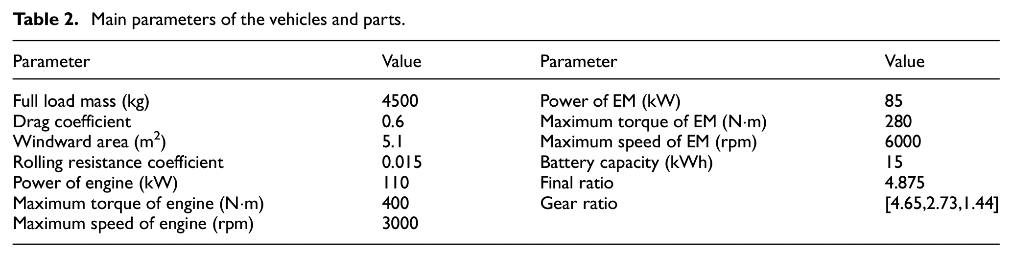
The research object of this paper is electric trucks driving a fixed route. A bus route in Xi’an, China, is taken as an example, as shown in Figure 1. Other information is uncertain, it depends on traffic conditions and can be regarded as stochastic. For this, speed profiles are obtained from 50 driving tests, as shown in Figure 2. The relevant information statistics of the daily route are shown in Table 1. The parameters of the vehicle and parts are shown in Table 2. Since the route is fixed, historical data can be effectively utilized to design control strategies. MPC requires prediction of future road information, and is currently divided into two types: deterministic prediction and stochastic prediction. This section describes the optimal control problem in discrete space for DMPC and SMPC, respectively. How to solve these problems will be discussed in detail in sections “Deterministic prediction and DMPC” and “Stochastic prediction and SMPC.”

Figure 1.

A driving route and corresponding altitude in Xi’an, China. In the top plot, location A and B denotes the start and end position, respectively. The bottom plot shows the profile of altitude from A to B.

Figure 2.

The speed profiles of historical driving tests.

Table 1.

Statistical information of the fixed driving route.

Parameter	Value
Length of route (km)	35.5
Average speed (km/h)	36.5
Maximum speed (km/h)	100.3
Average acceleration (m/s²)	0.608
Average deceleration (m/s²)	0.348
Maximum acceleration (m/s²)	4.2
Maximum deceleration (m/s²)	4.47

Table 2.

Main parameters of the vehicles and parts.

Parameter	Value	Parameter	Value
Full load mass (kg)	4500	Power of EM (kW)	85
Drag coefficient	0.6	Maximum torque of EM (N·m)	280
Windward area (m²)	5.1	Maximum speed of EM (rpm)	6000
Rolling resistance coefficient	0.015	Battery capacity (kWh)	15
Power of engine (kW)	110	Final ratio	4.875
Maximum torque of engine (N·m)	400	Gear ratio	[4.65,2.73,1.44]
Maximum speed of engine (rpm)	3000

PHEV model

The structure of the PHEV is shown is Figure 3, which is composed of an engine, an electric machine (EM), a clutch CL, and a gearbox.

Figure 3.

Mechanical structure of the HEV powertrain. The engine, EM, and the gearbox are connected in series on a shaft. The engine and EM are connected through the clutch CL.

According to Newton’s laws, the longitudinal dynamics of the vehicle can be described by Du et al.³⁶

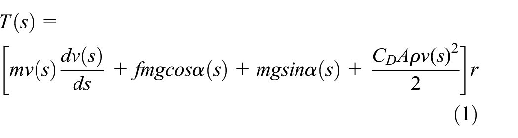
\begin{matrix} T (s) = \\ [mv (s) \frac{dv (s)}{ds} + fmgcos α (s) + mgsin α (s) + \frac{C_{D} A ρ v {(s)}^{2}}{2}] r \end{matrix}

(1)

where, T denotes the demand torque of the wheels; m denotes the mass of the vehicle; f is the rolling resistance coefficient; C_D is the air resistance coefficient; A is the windward area; g is the acceleration of gravity; α is the slope; v denotes the velocity of the vehicle.

Dynamic model (1) is built on the distance domain, in order to remove the nonlinearity, define

E = \frac{1}{2} v^{2}

(2)

where, E is kinetic energy of a unit mass.

The derivative of equation (2) can be obtained by

\frac{dE}{ds} = \frac{d v^{2}}{2 ds} = v \frac{dv}{ds}

(3)

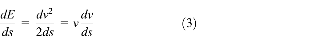
So, the kinetic equation (1) can be rewritten as:

\begin{matrix} T (s) = \\ [mv (s) \frac{dv (s)}{ds} + fmgcos α (s) + mgsin α (s) + C_{d} A_{f} ρ E (s)] r \end{matrix}

(4)

During driving, both the engine and the EM can provide driving force to the vehicle through the gearbox. When the CL is disengaged, the vehicle is fully driven by the EM. The state of the CL is represented by σ_c.

σ_{c} (s) \in {0, 1}

(5)

where, 0 and 1 denote the clutch is disengaged and engaged, respectively.

Further, the control action corresponding is denoted by

δ_{c} (s) \in {- 1, 0, 1}

(6)

So, the dynamics of CL is expressed by

σ_{c} (s^{+}) = σ_{c} (s) + δ_{c} (s)

(7)

Assuming that the operation state of the engine is the same as that of the clutch and ignore the on/off process of the engine, that is, when the clutch is disengaged, the engine is off; when the clutch is engaged, the engine is on. So, the torque of the engine can be described as

T_{e} (s) = {\begin{matrix} 0, σ_{c} (s) = 0 \\ \frac{T (s)}{f_{d} i_{g} (gear (s))} - T_{m} (s), σ_{c} (s) = 1 \end{matrix}

(8)

where, T_e and T_m denotes the output torque of the engine and EM, respectively; f_d and i_g(gear) denotes the gear ratio of the differential and gearbox, respectively; $gear \in {1, 2, 3, 4}$ denotes the gear of the gearbox.

Further, the shifting process of the gearbox is modeled by

gear (s^{+}) = gear (s) + shift (s)

(9)

where, $shift (s) \in {- 1, 0, 1}$ represent the three shift commands of downshift, unchanged, and upshift, respectively.

When the clutch is disengaged, the speed of the engine is zero, and when the clutch is engaged, the speed of the engine is equal to that of EM, that is,

ω_{e} (s) = σ_{c} (s) ω_{m} (s)

(10)

where, ω_e and ω_m denote the speed of the engine and EM, respectively.

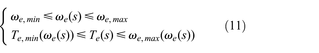
The PHEV adopts a diesel engine with a displacement of 2.5 L. The fuel consumption rate of the engine is denoted by m_f(s), as a nonlinear function of the speed and torque, which is shown in Figure 4. The constraints of the engine are as follows:

{\begin{matrix} ω_{e, \min} \leq ω_{e} (s) \leq ω_{e, \max} \\ T_{e, \min} (ω_{e} (s)) \leq T_{e} (s) \leq ω_{e, \max} (ω_{e} (s)) \end{matrix}

(11)

Figure 4.

Fuel consumption rate of the diesel engine versus torque and speed (unit: g/kWh).

The efficiency of EM is also modeled by a nonlinear function of speed and torque, which is shown in Figure 5. Define equation (2) to represent the power of EM, where P_d denotes the dissipated power of EM.

P_{m} (s) = T_{m} (s) ω_{m} (s) + P_{d} (T_{m} (s), ω_{m} (s))

(12)

Figure 5.

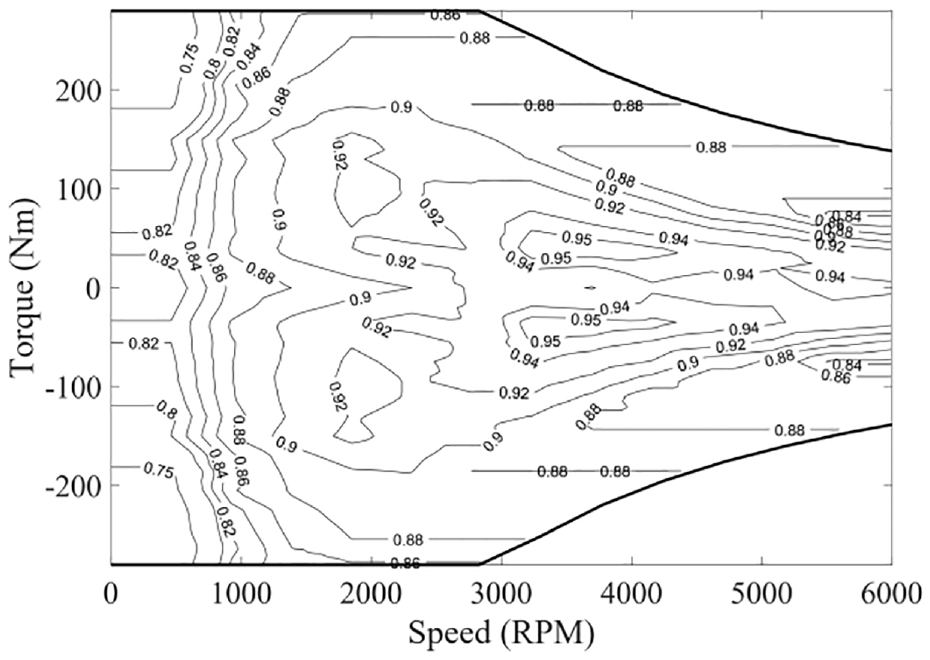
Efficiency of EM versus torque and speed.

The battery model adopts the equivalent circuit model. The $SOC$ of the battery is the ratio of the remaining capacity to the total capacity of the battery. The calculation formula of $SOC$ is as follows:

SOC = \frac{Q - \int_{0}^{t} i_{b} dt}{Q}

(13)

where, $Q$ is the rated capacity of the battery; $i_{b}$ is the charge and discharge current of the battery.

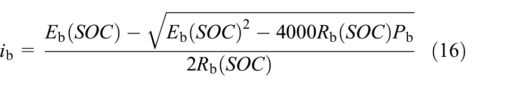
Battery charge and discharge power is

P_{b} = i_{b} U_{b}

(14)

where, $P_{b}$ is the charging or discharging power of the battery; $U_{b}$ is the terminal voltage of the battery, which can be obtained from the following formula:

U_{b} = E_{b} - i_{b} R_{b}

(15)

Among them, $E_{b}$ and $R_{b}$ are the electromotive force and internal resistance of the battery, The relation formula of battery circuit current is

i_{b} = \frac{E_{b} (SOC) - \sqrt{E_{b} {(SOC)}^{2} - 4000 R_{b} (SOC) P_{b}}}{2 R_{b} (SOC)}

(16)

Assuming that EM is the only electricity-consuming device in the vehicle, so P_bat = P_m. The power and SOC of battery also be constrained by

{\begin{matrix} | P_{bat} | \leq P_{B, \max} \\ SO C_{\min} \leq SOC \leq SO C_{\max} \end{matrix}

(17)

MPC problem description

In DMPC problem, the gear of gearbox, demand torque, and the SOC of battery are taken as the state variables; torque of EM, the state of CL, and shift action are taken as the control variables. In SMPC problem, the kinetic energy is taken as the stochastic variable considering the uncertainty of future traffic conditions. The order of state, control, and stochastic variables can be correspond to $u = [T_{m}, δ_{c}, shift]$ , $ω = E$ , and $x = [gear, σ_{c}, T, SOC]$ , respectively.

From a mathematical point of view, the MPC problem is to use a series of discrete control actions to optimize the performance indictors of vehicle driving within a certain time range. The performance indicators include fuel consumption and shift times.

For DMPC, the cost function in a sampling interval can be described as

J_{D} (x_{k}, u_{k}) = [T_{k} ω_{e}, k m_{f} (x_{k}, u_{k}) + β_{1} | shif t_{k} | + β_{2} | δ_{c}, k |] Δ s

(18)

For SMPC, the cost function is

\begin{matrix} J_{S} (x_{k}, u_{k}, ω_{k}) = \\ [T_{k} ω_{e}, k m_{f} (x_{k}, u_{k}, ω_{k}) + β_{1} | δ_{c}, k | + β_{2} | δ_{c}, k |] Δ s \end{matrix}

(19)

where, β₁ is a positive weight factor, which is used to limit the frequent shifting of the vehicle; β₂ is the penalty factor to prevent frequent start/stop of the engine; δ_s denotes the discrete interval of distance.

The objective of DMPC is to minimize the total cost in prediction horizon, which is described as

\underset{u_{k}}{minimize} \sum_{k = i}^{i + H_{p}} J (x_{k}, u_{k})

(20)

where, i is the index over entire driving process; k denotes the index over the prediction horizon.

Considering the uncertainty of future vehicle speed, the goal of SMPC is to minimize the expect cost in prediction horizon, which is described as

\underset{u_{k}}{minimize} E_{ω_{k + 1} ~ \tilde{f} (ω_{k}, k)} \sum_{k = i}^{i + H_{p}} J_{S} (x_{k}, u_{k}, ω_{k})

(21)

where, $\tilde{f} (ω_{k}, k)$ denotes the probability distribution of ω_k₊₁.

Both SMPC and DMPC need to satisfy a series of constraints, which is detailed as

ω_{e, \min} \leq ω_{e, k} \leq ω_{e, \max}

(22a)

T_{e, \min} (ω_{e}, k) \leq T_{e, k} \leq ω_{e, \max} (ω_{e}, k)

(22b)

ω_{m, \min} \leq ω_{m, k} \leq ω_{m, \max}

(22c)

T_{m, \min} (ω_{m}, k) \leq T_{m, k} \leq ω_{m, \max} (ω_{m}, k)

(22d)

| P_{bat, k} | \leq P_{b, \max}

(22e)

SO C_{\min} \leq SO C_{k} \leq SO C_{\max}

(22f)

Deterministic prediction and DMPC

This section reports a DMPC scheme for the PHEV. First, two deterministic speed predictors are introduced. Then, the solution for DMPC is introduced.

Since the historical data is continuous, which needs to be discretized before introducing the predictive models. Without loss of generality, the set $Ω = {{\hat{v}}_{y, k} | y \in {1, \dots, W}, k \in {1, \dots, L}}$ to represent the historical measurements, where ${\hat{v}}_{y, k}$ denotes the velocity measured at position k at the driving test y. Stochastic variable v is discretized as ${v^{1}, v^{2}, \dots, v^{8}}$ , where $v^{i} < v^{i + 1}, \forall i \in {1, \dots, s - 1}$ . Define $v^{0} = 2 inf {v, v \in Ω} - v^{1}, v^{s + 1} = 2 sup {v, v \in Ω} - v^{8}$ . Let $V_{i} = {v \in R : \frac{v^{i - 1} + v^{i}}{2} < v \leq \frac{v^{i} + v^{i + 1}}{2}}$ denote the interval corresponding to the state $v^{i}$ , for all $i \in {1, 2, \dots, s}$ . The processing of stochastic variable v will be used in both DMPC and SMPC.

ANN based predictor

Artificial neural network (ANN) has relatively strong nonlinear mapping ability, and can find the law of data. So, it has been widely used in driving information prediction. Here, the radial basis function (RBF) neural network are used to predict the future velocity, which consists of input layer, hidden layer, and output layer. In this study, the Gaussian function are chosen to active the neurons in the hidden layer, which is described as

f (X) = \exp (\frac{- | | X - c | |^{2}}{2 σ^{2}})

(23)

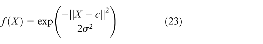
where, c and σ denote the neural net center and the spread width, respectively.

The input of the RBF is the trajectory of historical data, and the output is the predicted trajectory, which can be described as

[v_{N, k + 1}, \dots, v_{N, k + H_{p}}] = f (v_{k - H_{q + 1}, \dots,} v_{k})

(24)

where, H_q denotes the dimension of input vector; H_p denotes the length of prediction horizon; $v_{N, k}$ denotes the prediction value of speed.

An improved ANN based predictor

The accuracy of most predictive models relies primarily on historical data. In practical applications, the prediction error in the past short period indicates the gap between the prediction model and the actual situation, which can be effectively used to improve the prediction error. A reasonable assumption is that the offset between the prediction and measurement at current step is a good estimate of the offset in the short future. Based on this, an improved predictor is defined as

v_{D, k + 1} = {\begin{matrix} v_{N, k + 1} + λ (v_{k} - v_{D, k}), k = i \\ v_{N, k + 1} + λ (v_{D, k} - v_{N, k}), \\ k \in {i + 1, \dots, i + H_{p}} \end{matrix}

(25)

where, $v_{D, k}$ denotes the improved prediction value; $v_{k}$ denotes the measurement at step k; $v_{N, k}$ denotes the prediction value obtained from the ANN predictor described in equation (24); $0 \leq λ \leq 1$ models the damping of the influence of the current measurement in the future.

The improved predictor is based on the assumption that the offset between the measurement and the prediction has an impact on future prediction and that the impact will decay over time. It is clear that λ describes how the difference between $v_{D, k}$ and $v_{N, k}$ changes from one step to another.

λ = \frac{v_{D, k + 1} - v_{N, k + 1}}{v_{D, k} - v_{N, k}}, k \in {i + 1, \dots, i + H_{p}}

(26)

An example of prediction process is shown in Figure 6 to show the difference between equations (24) and (25). It can be seen that the offset between the two predicted trajectories will become smaller and smaller, and eventually coincide. The rate of decay depends on the value λ. The predictive trajectory of the vehicle speed according to equation (25) is denoted as

V_{D} = [v_{D, k}, v_{D, k + 1}, \dots, v_{D, k + H_{p}}]

(27)

Figure 6.

An example of the predicted trajectories, where Δ denotes the offset between measurement and prediction at step i. The blue and red lines denote the predicted trajectories generated by equations (21) and (22), respectively. It can be seen that Δ gradually decays in the prediction horizon, and the two predicted trajectories gradually overlap.

Dynamic programming for DMPC

The optimal problem described in section “MPC problem description” is nonlinear and mix-integer optimization problem. It is usually challenging to solve such problems in limited time. But the main contribution of this study is the novel predictors, we do not care the computation burden of the optimal policy. In this case, dynamic programming (DP) is the best option to test the performance of predictors.

First, a cost-to-go function $Φ_{D}^{π}$ is defined to represent the cost from current step to the end of prediction horizon according policy π, which can be detailed as

Φ_{D}^{π} (x_{i}, u_{i}) = \sum_{k = i}^{i + H_{p}} J_{D} (x_{k}, u_{k})

(28)

where, $u_{i}$ is the control action taken at state $x_{i}$ according to policy π.

So, the task of the optimal control problem is to get the minimum cost described in equation (28) and the corresponding control action, which can be described as

π^{*} (x_{i}) = \arg min_{u_{i}} Φ_{D}^{π} (x_{i}, u_{i})

(29)

where, $π^{*}$ denotes the optimal policy.

According to Bellman principle, equation (29) can be solved recursively

Φ_{D}^{π^{*}} (x_{i}, u_{i}) = min_{u_{i}} {Φ_{D}^{π^{*}} (x_{i + 1}, u_{i + 1}) + J (x_{i}, u_{i})}

(30)

Suppose the cost at the end of prediction horizon is 0, that is, $Φ_{D} (x_{i + H_{p}}, v_{i + H_{p}}) = 0$ . In each MPC update, after obtaining the optimal policy $π^{*}$ , its first value $π^{*} (x_{i})$ is used as the control action at current position.

Stochastic prediction and SMPC

The fundamental principle of SMPC is similar to that of DMPC, the main difference is that the strategy obtained by SMPC is statistically optimal. This section introduces a stochastic predictor and the solution method of SMPC.

A novel stochastic predictor

A novel stochastic predictor is proposed based on the deterministic predictor in Section “an improved ANN based predictor” First we need to model the uncertainty of future, which is usually difficult. In this study, we try to add a random term to the prediction model using the distribution of historical data along the driving route. The improved predictor is defined as

v_{S, k} = v_{D, k} + σ_{k} μ

(31)

where, $v_{S, k}$ denotes the improved predictive value; $v_{D, k}$ denotes the predictive value obtained from equation (25); µ is the random variable obeying the normal distribution N(0,1); σ_k is the standard deviation of the distribution of v at position k, which is calculated from historical data

{\begin{matrix} σ_{k} = \sqrt{\frac{1}{W} \sum_{l = 1}^{W} {(\hat{v} (y, k) - {\bar{v}}_{k})}^{2}} \\ {\bar{v}}_{k} = \frac{1}{w} \sum_{y = 1}^{w} {\hat{v}}_{y, k} \end{matrix}

(32)

The motivation of equation (31) is to better utilize the velocity distribution law at different locations. The predictive result of traditional predictors only depends on the previous measurements, while the prediction result of equation (31) depends not only on the previous measurements, but also on the historical measurements of position k along the route.

Stochastic dynamic programming for SMPC

Stochastic dynamic programming is a general algorithm to solve SMPC problem. Unlike DMPC, the goal of SMPC is to minimize the expectation of the cumulative cost in the prediction horizon.

Define equation (33) to represent the expectation of the cumulative cost in the prediction horizon.

Φ_{S}^{π} (x_{i}, u_{i}, w_{i}) = E_{w_{k + 1 ~ \tilde{f} (w_{k}, k)}} \sum_{k = i}^{i + H_{p}} J_{s} (x_{k}, u_{k}, w_{k})

(33)

where, $u_{i}$ denotes the control action for a given state and stochastic variables $(x_{i}, w_{i})$ according polity π.

The task of SMPC is to find the minimum of equation (33) and corresponding optimal policy $π^{*}$ , that is,

π^{*} (x_{i}, w_{i}) = \arg min_{u_{i}} Φ_{S}^{π} (x_{i}, u_{i}, w_{i})

(34)

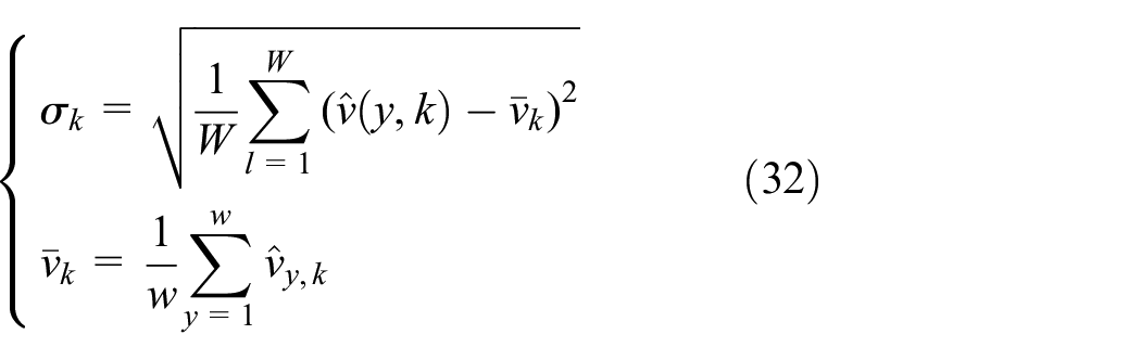
Considering the existence of the stochastic variable, the cost function at the next step can be regarded as conditional probability. For the stochastic predictor described in equation (31), the minimum expected cost function can be expressed as:

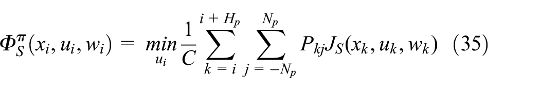
Φ_{S}^{π} (x_{i}, u_{i}, w_{i}) = \min_{u_{i}} \frac{1}{C} \sum_{k = i}^{i + H_{p}} \sum_{j = - N_{p}}^{N_{p}} P_{kj} J_{S} (x_{k}, u_{k}, w_{k})

(35)

where, 2N_p₊₁ is the number of available state of v. In order to unify the discrete space of v, let 2N_p₊₁ = w; P_kj is the possibility of transition from $v_{k}$ to $v_{k + 1} = v_{D, k + 1} + j σ_{k + 1}$ , which can be expressed as:

{\begin{matrix} P_{kj} = \frac{1}{\sqrt{2 π σ_{k}^{2}}} e^{- \frac{1}{2} \frac{{(v_{j} - v_{D, k})}^{2}}{σ_{k}^{2}}} = \frac{1}{σ_{k} \sqrt{2 π}} e^{- \frac{1}{2} j} \\ v_{j} = v_{D, k} + j σ_{k} \end{matrix}

(36)

The constant C normalizes the overall probability to 1.

C = \sum_{j = - N_{p}}^{N_{p}} \frac{1}{σ} \frac{1}{\sqrt{2 π}} e^{- \frac{1}{2} j}

(37)

Another difference between SMPC and DMPC is that online computation is not required. After the optimal policy $π^{*}$ is obtained, the set $(x_{i}, w_{i}, u_{i})$ are stored in the table. In real deployment, the optimal control action is obtained by looking up the table instead of online calculation.

Simulations and discussions

A comprehensive comparative analysis of the controllers using the proposed predictors is conducted by simulations in this section. DP is employed as the benchmark in this study. For ease of description, these control strategies are named as follows.

DMPC: DMPC with ANN based predictor.

DMPC: DMPC with the improved deterministic predictor described in equation (22).

SMPC: SMPC with the stochastic predictor described in equation (28).

DP: Dynamic programming, which is used as the benchmark assuming that the profile of speed is completely known. It is a global optimization algorithm which can obtain the optimal policy.

Parameters

The simulations was preformed on a personal computer (Intel i7-11800H at 2.3 GHz and RAM 16 GB), using MATLAB 2021a. Since the purpose of the simulation is to compare the performance of the predictors, computational burden is not taken into account. A small quantization resolution is chosen for continuous variables. The main parameters related to simulations are shown in Table 3.

Table 3.

Parameters of simulations.

Parameter	Value
Prediction horizon	100 m
Sampling interval	10 m
Quantization of the torque	5 N·m
Quantization of SOC	0.01
Quantization of v	1 km/h

Results and discussions

Table 4 summaries the results and cost benefit of the controller using proposed predictors. Compared with DMPC, I-DMPC has the 2.98% lower cost, SMPC has the 4.5% lower cost. This indicates that the improved predictors proposed in this paper can improve the performance of the controllers.

Table 4.

Results of simulation.

Strategy	DMPC	I-DMPC	SMPC	DP
Cost	3.11	3.02	2.97	2.93
Economy improvement		2.98%	4.5%	5.79%

One of the driving tests is chosen to compare the performance of the proposed predictors. The speed profile and the trajectory of gear shift during driving are shown in Figure 7. The top plot shows the velocity along the route. Remaining plots show the profiles of gear for different controllers. From the gear shifting trajectories of DMPC and I-DMPC, it can be seen that the shifting frequency of I-DMPC is significantly lower than that of DMPC in a short distance. For example, when the driving distance is between 10 and 12 km, due to frequent changes of vehicle speed, DMPC frequently switches between 3-rd and 4-th gears within a short distance, which will increase the wear of the clutch and reduce the driving comfort. Although I-DMPC has a high number of shifts between the driving distances of 10–15 km, the distance between two shifts longer than that of DMPC, and there is no frequent shift of shift of gears within a short distance. When the driving distance is between 10 and 11 km, DP mostly works in 4-th gear, while SMPC and I-DMPC switch between 2-nd, 3-rd, and 4-th gear, and DMPC switches between 3-rd and 4-th gear. This shows that the performance of the controllers using the predictors proposed in this paper still has a certain gap compared with DP in low-speed and complex road conditions. In high-speed route sections (e.g., 15–25 km), SMPC and DP always work in 4-th gear, and DMPC and I-DMPC switch between 3-rd and 4-th gear. This shows that the performance of SMPC at high speed is close to that of DP, but the performance of DMPC and I-DMPC at high speed still has a certain gap with DP.

Figure 7.

The driving test and the corresponding simulation results. The top plot shows the velocity along the route. Remaining plots show the profiles of gear for different controllers. It can be seen that the shifting frequency of SMPC is lower than DMPC and I-DMPC. In high-speed conditions (15–25 km), SMPC always works in 4-th gear, which is closest to DP.

The trajectories of engine state of different controllers are shown in Figure 8. As can be seen, all four controllers prefer to keep the engine running under high-speed road conditions. This is because the operating points of the engine corresponding to the high-speed road conditions are usually in the high-efficiency operation range, and the performance of the controllers in high-speed road conditions is close to that of DP. Compared with SMPC and I-DMPC, DMPC has more engine switching times, but the fuel consumption is not reduced. This shows that the performance of the predictive model used by DMPC is poor, resulting in frequent engine state-stop switching without reducing fuel consumption. Compared with SMPC and I-DMPC, DP also has more number of engine state-stop switching, but the total cost is also the least. Since DP represents the global optimal strategy, this shows that there is a contradiction between the minimum number of engine state-stop switching and the lowest fuel consumption, and the optimality cannot be achieved at the same time. In practical applications, the appropriate penalty factor for engine state-stop switching should be determined according to specific needs.

Figure 8.

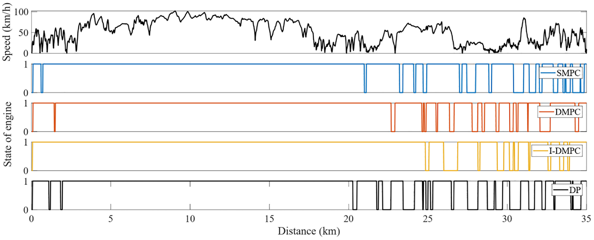
Trajectories of engine state of different controllers. The top plot shows the velocity along the route. Remaining plots show the profiles of engine state of different controllers.

The SOC trajectories of different controllers during the driving test are shown in Figure 9. It can be seen that the trajectory of SMPC is closest to DP. This shows that considering the distribution law of historical vehicle speed at different locations can effectively improve the performance of the predictor. The SOC trajectory of DMPC is at the top at 0–20 km, which shows that the control strategies using the prediction models proposed in this paper prefer to use battery energy for driving than DMPC when the electric power is sufficient, which can save fuel consumption. The SOC trajectory of I-DMPC at 0–10 km is at the bottom, which shows that I-DMPC prefers to use battery energy than DP and SMPC. However, the driving cost of I-DMPC is higher than that of DP and SMPC, which means that from the perspective of the minimum cost of the entire route, even when the battery is sufficient, the proportion of battery energy to total energy should be kept within an appropriate range. Using too much or too little energy from the battery will drive the control strategy away from the global optimum.

Figure 9.

Trajectories of SOC of different control strategies during the driving test. It can be seen that the trajectory of SMPC is closest to DP.

The operating points of the engine of different controllers are shown in Figure 10. It can be seen that the sets of operation pointes of SMPC are the closest to DP and concentrated in the efficient area. Operation points of I-DMPC are also denser than DMPC. Engine of DMPC operates in more dispersed area, which results in their poorer performance.

Figure 10.

Operating points of engine during the driving test. The sets of operation points of DP are densest. Operation points of SMPC are closest to DP. DMPC operates in the largest area, which results higher cost.

Conclusion

To improve the performance of MPC energy management strategies of PHEVs, this paper develops a deterministic predictor for DMPC and a stochastic predictor for SMPC. For DMPC, the neural network-based predictor is first introduced and taken as the benchmark predictor. A novel deterministic predictor considering historical prediction errors is proposed, which relies on the assumption that the offset between the prediction and measurement at current instant is a good estimate of the offset in the short future. Based on the proposed deterministic predictor, a stochastic predictor that considers the distribution law of historical data at different locations is further proposed.

Simulation results show that the controller using the proposed deterministic predictor improves fuel economy by 2.98% compared with the benchmark. The controller using the proposed stochastic predictor improves fuel economy by 4.5% compared with the benchmark.

The proposed two strategies can be used as a high-level controller providing the control commands for underlying controller such as electronic control units of the engine and the powertrain. Future work will focus on two aspects: (1) Generalizing the proposed control strategies to the eco-driving problem of arbitrary routes; (2) Implementing proposed control strategies in a truck and testing the performance in real traffic.

Footnotes

Handling Editor: Chenhui Liang

Declaration of conflicting interests

The author(s) declared no potential conflicts of interest with respect to the research, authorship, and/or publication of this article.

Funding

The author(s) disclosed receipt of the following financial support for the research, authorship, and/or publication of this article: This work was supported by the National Natural Science Foundation of China (U1937203), State Key Laboratory for Mechanical Behavior of Materials (1991DA105206), Young Talent Fund of Association for Science and Technology in Shaanxi, China (20240432), and Shaanxi Province Science and Technology Activities for Overseas Students Selected Funding Project (2023-007).

ORCID iDs

Jingzhou Gao

Wei Du

References

Agamloh

von Jouanne

Yokochi

. An overview of electric machine trends in modern electric vehicles. Machines 2020; 8: 20.

Hannan

Azidin

Mohamed

. Hybrid electric vehicles and their challenges: a review. Renew Sustain Energy Rev 2014; 29: 135–150.

Chan

. The state of the art of electric, hybrid, and fuel cell vehicles. Proc IEEE 2007; 95: 704–718.

Han

Tang

, et al. Powertrain design and control in electrified vehicles: a critical review. IEEE Trans Transp Electrif 2021; 7: 1990–2009.

Jiang

Egardt

, et al. Advanced power-source integration in hybrid electric vehicles: multicriteria optimization approach. IEEE Trans Ind Electron 2015; 62: 7847–7858.

Huang

Wang

Khajepour

, et al. Model predictive control power management strategies for HEVs: a review. J Power Sources 2017; 341: 91–106.

Ali

Moulik

. On the role of intelligent power management strategies for electrified vehicles: a review of predictive and cognitive methods. IEEE Trans Transp Electrif 2022; 8: 368–383.

Zhao

Jin

, et al. Parameter optimization of rule-based control strategy for multi-mode hybrid electric vehicle. Proc Inst Mech Eng D J Automob Eng 2020; 234: 2706–2716.

Lin

Peng

Grizzle

, et al. Power management strategy for a parallel hybrid electric truck. IEEE Trans Control Syst Technol 2003; 11: 839–849.

10.

Sciarretta

Back

Guzzella

. Optimal control of parallel hybrid electric vehicles. IEEE Trans Control Syst Technol 2004; 12: 352–363.

11.

Maino

Misul

Musa

, et al. Optimal mesh discretization of the dynamic programming for hybrid electric vehicles. Appl Energy 2021; 292: 116920.

12.

Murgovski

Johannesson

, et al. Optimal dimensioning and power management of a fuel cell/battery hybrid bus via convex programming. IEEE/ASME Trans Mechatron 2015; 20: 457–468.

13.

Choi

M-E

Kim

S-W

Seo

S-W

. Energy management optimization in a battery/supercapacitor hybrid energy storage system. IEEE Trans Smart Grid 2012; 3: 463–472.

14.

Ghandriz

Jacobson

Murgovski

, et al. Real-time predictive energy management of hybrid electric heavy vehicles by sequential programming. IEEE Trans Vehicular Technol 2021; 70: 4113–4128.

15.

Serrao

Onori

Rizzoni

. ECMs as a realization of Pontryagin’s minimum principle for HEV control. In: 2009 proceedings of the American control conference, St Louis, MO, USA, 10–12 June 2009, vols 1–9, pp. 3964–3969. New York: IEEE.

16.

Kim

Cha

Peng

. Optimal control of hybrid electric vehicles based on Pontryagin’s minimum principle. IEEE Trans Control Syst Technol 2011; 19: 1279–1287.

17.

Tang

Rizzoni

Onori

. Energy management strategy for HEVs including battery life optimization. IEEE Trans Transp Electrif 2015; 1: 211–222.

18.

Pisu

Rizzoni

. A comparative study of supervisory control strategies for hybrid electric vehicles. IEEE Trans Control Syst Technol 2007; 15: 506–518.

19.

Zeng

Zhang

, et al. Optimization-oriented adaptive equivalent consumption minimization strategy based on short-term demand power prediction for fuel cell hybrid vehicle. Energy 2021; 227: 120305.

20.

Tate

Grizzle

Peng

. SP-SDP for fuel consumption and tailpipe emissions minimization in an EVT hybrid. IEEE Trans Control Syst Technol 2010; 18: 673–687.

21.

Zeng

Wang

. A parallel hybrid electric vehicle energy management strategy using stochastic model predictive control with road grade preview. IEEE Trans Control Syst Technol 2015; 23: 2416–2423.

22.

Sun

Moura

, et al. Velocity predictors for predictive energy management in hybrid electric vehicles. IEEE Trans Control Syst Technol 2015; 23: 1197–1204.

23.

Guo

Yang

. Predictive energy management for dual-motor BEVs considering temperature-dependent traction inverter loss. IEEE Trans Transp Electrif 2022; 8: 1501–1515.

24.

Zhang

Huang

Chen

, et al. A novel learning-based model predictive control strategy for plug-in hybrid electric vehicle. IEEE Trans Transp Electrif 2022; 8: 23–35.

25.

Greenwell

Vahidi

. Predictive control of voltage and current in a fuel cell-ultracapacitor hybrid. IEEE Trans Ind Electron 2010; 57: 1954–1963.

26.

Borhan

Vahidi

Phillips

, et al. MPC-based energy management of a power-split hybrid electric vehicle. IEEE Trans Control Syst Technol 2012; 20: 593–603.

27.

Liu

Wang

, et al. Hybrid electric vehicle downshifting strategy based on stochastic dynamic programming during regenerative braking process. IEEE Trans Veh Technol 2018; 67: 4716–4727.

28.

Liu

Gao

, et al. Prediction of vehicle driving conditions with incorporation of stochastic forecasting and machine learning and a case study in energy management of plug-in hybrid electric vehicles. Mech Syst Signal Process 2021; 158: 107765.

29.

Borhan

Vahidi

Phillips

, et al. Predictive energy management of a power-split hybrid electric vehicle. In: Proceedings of the American Control Conference, 2009, St Louis, MO, USA, 10–12 June 2009, vols 1–9, pp. 3970+. New York: IEEE.

30.

Amini

Kargarian

Karabasoglu

. ARIMA-based decoupled time series forecasting of electric vehicle charging demand for stochastic power system operation. Electr Power Syst Res 2016; 140: 378–390.

31.

Moura

Fathy

Callaway

, et al. A stochastic optimal control approach for power management in plug-in hybrid electric vehicles. IEEE Trans Control Syst Technol 2011; 19: 545–555.

32.

Gross

Wittwer

Diehl

. Stochastic model predictive control of photovoltaic battery systems using a probabilistic forecast model. Eur J Control 2020; 56: 254–264.

33.

Chen

. Robust multiagent reinforcement learning toward coordinated decision-making of automated vehicles. SAE Int J Veh Dyn Stab NVH 2023; 7: 475–488.

34.

Hou

Yang

, et al. Active vibration control of electric drive system in electric vehicles based on active disturbance rejection current compensation under impact conditions. SAE Int J Veh Dyn Stab NVH 2023; 7: 513–531.

35.

Raabe

Fontana

Neubeck

, et al. Contribution to the objective evaluation of combined longitudinal and lateral vehicle dynamics in nonlinear driving range. SAE Int J Veh Dyn Stab NVH 2023; 7: 533–554.

36.

Murgovski

, et al. Stochastic model predictive energy management of electric trucks in connected traffic. IEEE Trans Veh Technol 2022; 99: 1–13.

Deterministic and stochastic model predictive energy management of hybrid electric vehicles using two improved speed predictors

Abstract

Keywords

Introduction

Problem formulation

Driving scenario

PHEV model

MPC problem description

Deterministic prediction and DMPC

ANN based predictor

An improved ANN based predictor

Dynamic programming for DMPC

Stochastic prediction and SMPC

A novel stochastic predictor

Stochastic dynamic programming for SMPC

Simulations and discussions

Parameters

Results and discussions

Conclusion

Footnotes

Declaration of conflicting interests

Funding

ORCID iDs

References