
Abstract
The suspension system plays a critical role in automobiles, ensuring the safety and comfort of vehicle occupants. However, extended usage, varying road conditions, external forces, and heavy loads can result in damage and faults within the internal components of the suspension system. To mitigate the occurrence of suspension system failures, the development of an effective fault diagnosis system for suspension components becomes imperative. Traditional fault diagnosis techniques often heavily rely on human expertise, which comes with certain limitations. In response, researchers have embraced intelligent fault diagnosis techniques, with transfer learning-based fault diagnosis emerging as a highly effective approach. By leveraging transfer learning, it becomes possible to extract and select fault-specific features for classification purposes. Deep learning-based methods, with their capacity to extract significant features and essential information from raw data, offer notable advantages. Despite these advantages, the implementation of deep learning-based fault diagnosis in suspension systems remains relatively unexplored and limited. In this article, a deep transfer learning architecture specifically designed for fault diagnosis in suspension systems is proposed. The approach involves employing 12 pre-trained networks and tuning them to identify the optimal model for fault diagnosis. Time domain vibration signals obtained from suspension systems under seven fault conditions and one good condition are transformed into spectrogram images. These images are then pre-processed and used as input for the pre-trained networks in fault classification. The results demonstrate that among the 12 pre-trained networks, AlexNet outperforms the others in terms of classification accuracy while requiring the least amount of training time. Therefore, AlexNet network in conjunction with the spectrogram images of time domain vibration signals for applications in suspension system fault diagnosis is highly recommend.
Keywords
Introduction
Urbanization and population growth have made transportation an integral aspect of people’s daily lives. Individuals rely on different modes of transportation, including air travel, water transport, and road transport. Among these options, road transport is favored by a vast majority. 1 Road transport encompasses various modes such as motorcycles, passenger cars, and public transportation systems like buses and railways. Among these, passenger cars are favored for their speed, convenience, safety, and comfort, making them the preferred choice for travel. In the era of urbanization, despite changing market dynamics, the sales of passenger cars have witnessed an annual increase of 18%.
When selecting a car as the primary mode of road transport, safety and comfort are the primary considerations. It is worth noting that road transport is often regarded as one of the most hazardous means of commuting. The combination of high speeds and heavy weights (ranging from 10 to 40 tons) of objects being transported contributes to the perceived dangers. The main cause of major road accidents can be attributed to the loss of directional stability or the reduction in road grip between the wheels and the road surface. 2 The stability of a vehicle, both during turns (lateral direction) and while moving straight (longitudinal direction), relies on the road grip it maintains. The grip between tires and road is directly influenced by the performance of suspension components and dampers. Any degradation in the performance of these elements can have significant consequences. The deterioration of suspension performance can result in a 12% increase in braking time and a 30% increase in braking distance. These effects, in turn, have a direct impact on the ride comfort experienced by occupants and can also affect the overall lifespan of the vehicle’s body. 3 During road transportation, automobiles encounter various disturbances, such as uneven road surfaces, centrifugal force during cornering, and acceleration and braking forces. These disturbances can cause discomfort to both the occupants and the driver, ultimately impacting the maneuverability of the vehicle. To mitigate the resulting vibrations, a passive suspension system is employed, consisting of hydraulic shock absorbers, lower arm tie rod, stabilizer bar, and coil springs that dissipate energy in terms of heat.
The suspension system plays a crucial role in ensuring safety and providing comfort in modern automobiles. While active and semi-active suspensions have gained significant attention in the past decade, research on passive suspension systems has been limited. The dominance of passive suspension systems in the automobile industry can be attributed to their high reliability, simple structure, and cost-effectiveness. Despite advancements in technology, passive suspension systems continue to be the preferred choice due to their reliable performance, straightforward design, and economic feasibility.4–6 Suspension system components are susceptible to various faults that arise from prolonged operation under different road conditions and loads. Factors such as wear, manufacturing defects, fatigue, misalignment, external damage, improper fitment, corrosion, and variations in wheel pressure contribute to the manifestation of faults in the suspension system. Consequently, internal components such as Damper with spring (strut), ball joint, and lower arm bush are prone to failure. The presences of these faults significantly impact the overall operation of the suspension system, raising concerns regarding safety and comfort. To mitigate the risk of fatal accidents and sudden breakdowns, it becomes essential to identify faults in the suspension system. Traditional fault diagnosis methods either they use model-based approach or data driven approach. In order to perform model-based fault diagnosis one has to have domain expertise in order to derive the faults from mathematical model or Finite elements the performance of these fault diagnosis using model-based approach relays on human expertise. Hence, data driven approach is been used widely. The approach involves a series of steps, including data acquisition, feature extraction, feature selection, and classification. In the initial step of data acquisition, various signals such as vibration, pressure, temperature, strain, speed, and acoustic are gathered. Among these, vibration signals are widely utilized in fault diagnosis systems for mechanical systems, as they exhibit intrinsic characteristics that reflect the condition of the machinery. Table 1 provides list of state of art fault diagnosis method used in the suspension system.
State of art fault diagnosis in suspension system.

From Table 1, one can identify the following research gaps: traditional methods lack studies involving multiple-component fault diagnosis. Moreover, the performance of state-of-the-art fault diagnosis using a model-based approach heavily depends on domain expertise to derive mathematical models, and these experiments are typically conducted in controlled environments. Lastly, there is a notable absence of research exploring the potential of machine learning in the domain of suspension system fault diagnosis. This research gap emphasizes the need for more efficient and automated approaches; hence, the focus has shifted to a machine learning approach.
In Machine learning approach to extract useful information from these signals, a range of features is employed, including statistical features, wavelet features, and histogram features. Moreover, optimization and dimensionality reduction techniques, such as feature clustering methods, genetic algorithms (GA), particle swam optimization (PSO), simulated annealing (SA), and principal component analysis (PCA), are applied to select the significant features from the available set. These methods aid in the selection of key features that provide valuable insights for fault diagnosis and ensure the safety, reliability, and comfort of the vehicle.9,14 Finally, using those significant features and machine learning algorithm, the fault classification of the system is carried out. In general decision trees, Self organizing map, K Nearest network, Support vector machines (SVM), neural networks (NN), Naïve Bayes are the widely used machine learning algorithm for fault classification of mechanical systems.15,16
The effectiveness of a specific fault diagnosis technique heavily relies on the type of features extracted from the acquired signals. Choosing the suitable extraction method for a particular dataset necessitates prior domain knowledge and a comprehensive understanding. Moreover, conventional feature extraction methods hinder the exploration of novel features as they heavily rely on existing features and evaluation criteria. Additionally, the techniques of feature extraction are highly sensitive to variations in the mechanical characteristics of a system. Considerable time and effort have been dedicated to identifying suitable feature extraction techniques for various fault diagnosis applications. Complex mathematical modeling and challenging feature extraction have posed significant challenges for conventional fault diagnosis techniques. Therefore, it is both meaningful and timely to develop an autonomous fault diagnosis technique that eliminates the need for domain expertise. This technique would automatically adapt the process of feature engineering (extraction and selection) on the acquired signals and adjust to changes in the mechanical characteristics of a system that occur during dynamic operation.
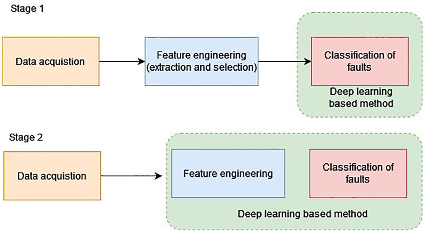
In recent times, the progress in computational devices and the abundance of data resulting from the adoption of “Industry 4.0” and “Internet of Things (IoT)” have garnered considerable interest from researchers. The field of artificial intelligence (AI) has experienced a surge in popularity in the realm of big data processing, opening up new avenues for fault diagnosis exploration. Modern intelligent fault diagnosis techniques are rooted in AI principles, particularly leveraging deep learning, which was introduced by Hinton et al. in the scientific community. Deep learning, also known as deep neural networks (DNN), employs a hierarchical structure with multiple neural layers to extract information from input data. This “deep” architecture allows for gradual extraction of raw data information, enabling the discovery of intricate dataset structures and automatic acquisition of significant features. Deep learning models find wide application in various domains such as NLP (natural language processing), face/object detection, pattern recognition, and robotics, owing to their ability to autonomously learn features and enhance non-linear regression. The utilization of deep neural networks (DNN) with their self-learning capabilities for fault diagnosis in mechanical systems is of great significance and holds immense potential. The process of fault diagnosis in mechanical systems, using deep learning, consists of two stages that rely on the intricate feature learning capabilities of DNN, as illustrated in Figure 1.
Deep learning stages in application of mechanical systems.
The two stages of deep learning application:
In recent years, researchers have been incorporating DNN into fault diagnosis, focusing on either classification or feature selection. The initial approach involved extracting acquired signal features using various techniques to train DNN models and evaluate their effectiveness following traditional fault diagnosis methods. This approach has been reported on by several authors, such as Lu et al., who proposed using a deep belief network to diagnose bearing and gearbox states using statistical features extracted from frequency, time, and time-frequency domains signals. 17 Similarly, Chen et al. proposed a model for detecting faults in gearboxes using a convolutional neural network (CNN) that incorporates frequency and time domain features. 18 During this stage of fault diagnosis, deep neural networks were initially explored as alternatives to traditional methods, but the full potential of DNN feature learning capabilities had not yet been fully realized (Figure 1 (Stage 1)).
During this stage, researchers adopted a combined approach that involved both feature extraction and classification of vibration data, whether in the form of raw signals or stored as images. This technique eliminated the need for domain expertise and reduced the time required for manual computations. The literature discussing this combined approach is discussed below. In their study, Grezmak et al. performed condition monitoring of roller bearings using deep convolutional neural networks on image data obtained from high-speed videos. They employed a CNN model for feature extraction and recognition of fault patterns. 19 Similarly, Zhao et al. utilized a convolutional long short-term memory (C-LSTM) network for tool condition monitoring. 20 Recently, Sai et al., adopted several pre-trained networks to classify various suspension faults using radar plots. 21 Furthermore, various optimization algorithms are present to enhance the performance of the networks. 22 The feature learning capability of DNNs has enabled the process of intelligent fault diagnosis to become more reliable and effective (Figure 1 (Stage 2)).
A convolutional neural network (CNN) is an advanced deep learning model employed for extracting and comprehending intrinsic features from image data. It has found extensive applications in analyzing unstructured data, including natural language processing and image detection. However, its utilization in diagnosing faults within mechanical systems, particularly in the context of suspension system fault diagnosis, has been relatively limited. Table 2 presents examples of fault diagnosis studies in mechanical systems that utilize a deep neural network approach.
Literatures on mechanical system using deep learning approach.

In this particular investigation, the effectiveness of 12 pre-trained networks in diagnosing the condition of a suspension system is assessed. Spectrogram images, generated from vibration signals, were employed for this purpose. To fine-tune the hyperparameters, including the train-test split ratio, batch size, optimizer (solver), and learning rate, random search optimization techniques is employed on these pre-trained networks. Subsequently, the results obtained were thoroughly analyzed and organized in a table to determine the most suitable network for detecting faults within the suspension system.
The present study was aimed to detect faults in various suspension components, specifically focusing on the worn-out ball joint in the tie rod and lower arm, strut mount failure, strut wear, low tire pressure, worn-out lower arm bush, and external strut damage. Vibration signals were acquired for these faulty components, along with a sample representing a good condition. Subsequently, these vibration signals were utilized to generate spectrogram images, which served as inputs for 12 pre-trained neural networks, namely AlexNet, VGG19, ResNet-50, ResNet101, DenseNet201, MobileNetV2, GoogLeNet, InceptionV3, InceptionResNetV2, Xception, VGG-16, and ShuffleNet. In order to enhance the efficiency of the pre-trained networks, various adjustments were implemented on hyperparameters such as batch size, solver, learning rate, and train-test split ratio. These modifications were evaluated to assess the performance of the pre-trained networks. Finally, the most efficient pre-trained network was chosen for real-time application for suspension fault diagnosis. Thus, the proposed method introduces the following innovations, addressing the earlier mentioned research gap and enhancing the fault diagnosis using a machine learning approach:
Deep learning utilization: This study advocates for the adoption of deep learning over traditional fault diagnosis methods, reducing human involvement in the feature engineering process. Deep learning improves automatic feature extraction, saving time, and enhancing fault diagnosis accuracy.
Multi-fault diagnosis: In contrast to studies concentrating on single component failures, this method identifies multiple faults online using only a single vibration sensor.
Pretrained network for suspension faults: This method pioneers the application of a pretrained network to identify multiple faults in the suspension system.
Spectrogram images for pretrained network: The paper suggests incorporating spectrogram images as inputs for the pretrained network.
This innovative approach advances fault detection by utilizing both temporal and frequency domain information, thereby increasing the model’s robustness.
Experimental studies
This section focuses on the test setup used in the study, the method of data collection, and the types of suspension faults examined. The test setup employed a quarter-car model to simulate the actual operation of a suspension system. To collect vibration signals from the test setup, an accelerometer was securely attached to the control arm of the McPherson suspension system using an adhesive technique. The procedure for acquiring vibration signals for different fault conditions involved replacing healthy suspension components with faulty ones, while ensuring that the remaining components remained in a sound state. A total of eight different classes of signals were collected, encompassing seven fault conditions and one signal representing a good condition. The complete methodology for diagnosing faults in the suspension system is illustrated in Figure 2.

Fault diagnosis methodology of suspension system using CNN.
Experimental setup
For this study, unused left-hand suspension system taken from a Hyundai i10 car is utilized to fabricate the experimental setup. Figure 3 shows the test setup designed for this study, which consists of the McPherson suspension system along with the driving mechanism and load mechanism. The main objective of this test setup was to gather vibration signals for various faults in the suspension components while the car was moving on a smooth surface at a consistent speed. The structure was constructed in such a way that the driving mechanism (motor and transmission system) would rotate the wheel at a consistent speed, assisted by two supporting idler rollers. To minimize undesired excitation or vibration transmitted to the system, the torque from the motor was transmitted to the wheel through a constant velocity joint (CV) and belt drives. To vary the force acting on the suspension system, a loader mechanism consisting of an idler roller, guide pillar, and a hydraulic jack was used. The hydraulic jack could lift the idler roller against the suspension system with the support of the guide pillars. Additionally, the hydraulic jack was equipped with a pressure gauge to indicate the force acting on the suspension system. In this particular study, a no load condition is considered, that is idler rollers are merely touching the tire without any additional load is being applied so that there is no physical movement is seen in pressure gauge provided.
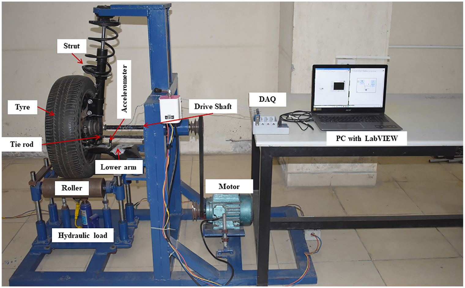
Experimental setup of McPherson suspension system.
Data acquisition
Data acquisition involves the conversion of analog information from the surrounding environment into digital values that can be processed, analyzed, and stored on a computer. In this particular study, the diagnosis of suspension system faults was conducted by utilizing an accelerometer, specifically a piezoelectric sensor. The accelerometer was affixed to the lower arm of the suspension system using an adhesive method. To facilitate the conversion from analog to digital, the analog vibration signals underwent conditioning and were then transformed into digital format using the NI9234 DAQ system. This system received input from the accelerometer’s output via a USB chassis. The digital values obtained were acquired and stored in the computer using the NI LabVIEW software. During the signal collection process, certain parameters were configured. The sampling length was set to 10,000 steps, while the frequency was set to 25 kHz. Additionally, the data collection process was conducted for no load conditions, with each fault condition consisting of 100 instances.
Faults in suspension system
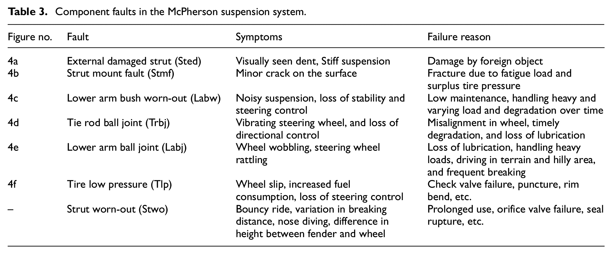
The suspension system plays a crucial role in ensuring the safety and comfort of vehicle occupants. It comprises several components, including the strut (consisting of a damper and coil spring), lower arm, tie rod, strut mount, and knuckle, which work together to form a cohesive suspension system. During normal driving conditions, the suspension system is exposed to dynamic loads that occur throughout its operation. Various factors can contribute to the development of faults within the suspension components. These include extended usage, insufficient maintenance, improper tire pressure, and the gradual degradation of internal components over time. When faults manifest in the suspension system, they diminish its overall performance, resulting in reduced reliability and comfort for the occupants. A visual representation of the faults present in the suspension components can be seen in Figure 4. Table 3 provides a concise overview of the different types of faults that can occur within these components.
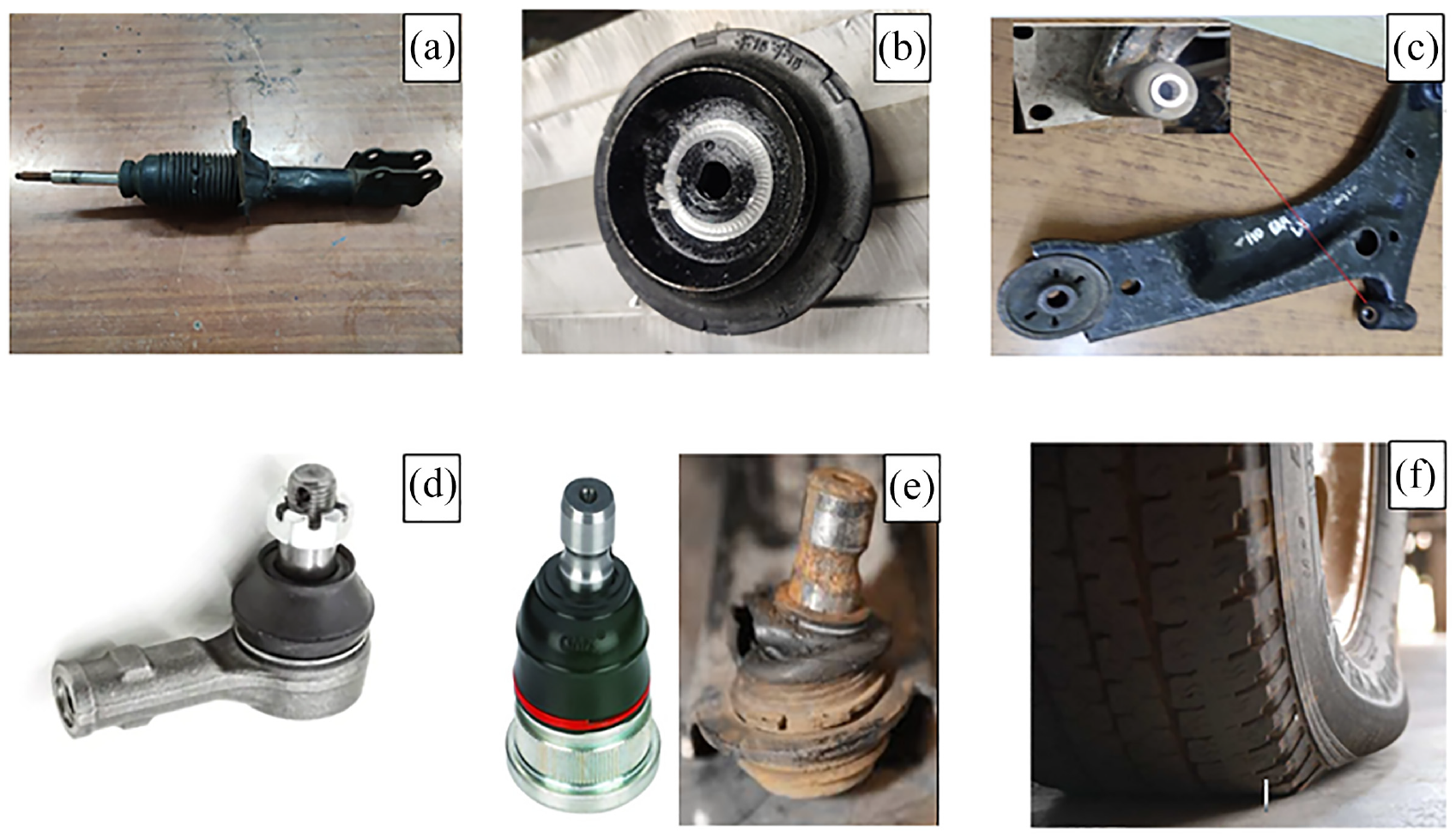
Various faults in the suspension system: (a) external damaged strut (Sted), (b) strut mount fault (Stmf), (c) lower arm bush worn-out (Labw), (d) tie rod ball joint (Trbj), (e) lower arm ball joint (Lanj), and (f) tire low pressure (Tlp).
Component faults in the McPherson suspension system.
Description of convolutional neural networks (CNN)
CNN, which stands for Convolutional Neural Network, is a powerful machine learning technique based on deep learning algorithms. It excels at analyzing input images by assigning importance (weights and biases) to various features and successfully distinguishing between them. The CNN architecture comprises three primary layer groups: the input layer, convolution layer, pooling layer, and fully connected layer. Figure 5 illustrates a fundamental form of CNN architecture. The function of each layer in the CNN architecture is described below:
(a) The first layer, known as the input layer, receives the image input in the form of pixel values.
(b) The convolution layer calculates the output of neurons connected to the input layer by performing the dot product between the weights and the input volume. The rectified linear unit (ReLU) activation function is then applied to enhance the activation output obtained from the previous layer. 26
(c) The pooling layer performs down sampling on the inputs, reducing their spatial dimensionality. This process helps to decrease the number of parameters while retaining the activation function.
(d) The fully connected layer, also known as the dense layer, is employed to capture intricate relationships between features by performing a dot product and applying an activation function such as softmax or sigmoid. It is commonly used for classification tasks, contributing to the overall classification performance of the neural network.
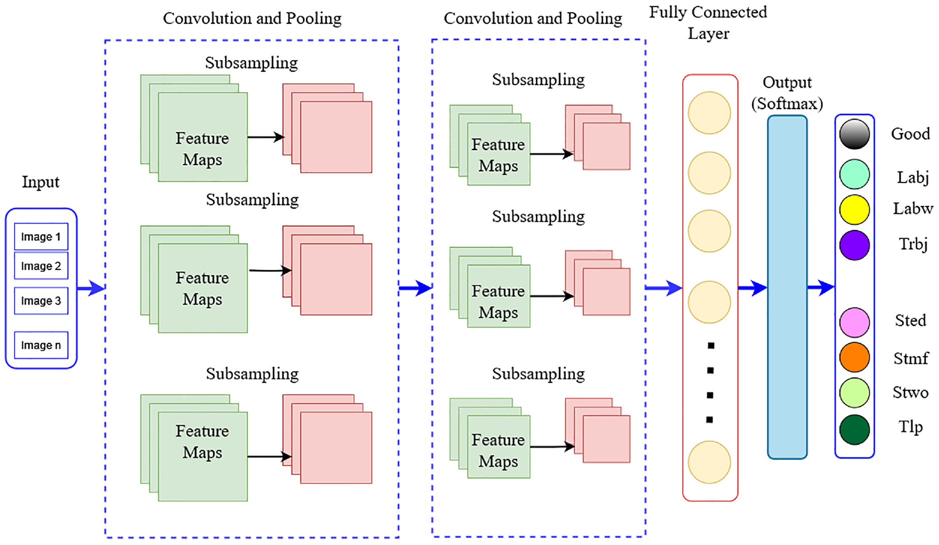
General architecture of convolutional neural networks.
Convolutional neural networks (CNNs) utilize convolutional and down sampling techniques to transform the initial input layer into class scores for regression and classification purposes. Thus, it is important to know that the designing the overall architecture of a CNN alone is insufficient. Developing and refining these models can be time-consuming. Therefore, it is necessary to carefully examine each layer’s hyper parameters and connectivity to gain a comprehensive understanding of how they function. Hence, in the following section, discusses about preprocessing techniques and hyper parameter tuning process.
Fault diagnosis in suspension system using pre-trained networks
The following section discusses the utilization of pre-trained networks in the current study for diagnosing faults in suspension systems. Initially, the acquired vibration signals are converted into images, which are then subjected to pre-processing and resizing to either 224 × 224 or 227 × 227, depending on the requirements of the chosen pre-trained network. The study incorporates 12 pre-trained networks, namely AlexNet, GoogLeNet, VGG-16, VGG-19, ResNet-50, ResNet-101, DenseNet-201, MobileNetV2, InceptionV3, InceptionResNetV2, Xception, and ShuffleNet. These networks are employed to classify the images and determine the condition of the suspension system. Transfer learning is applied in this research, where the initial weights of the networks, trained on the ImageNet dataset, are utilized. To adapt the networks to a specific dataset, the final output layers are replaced with new layers that correspond to the desired number of user-defined classes. Figure 6 presents an overview of the complete workflow for fault diagnosis in suspension systems using pre-trained networks.
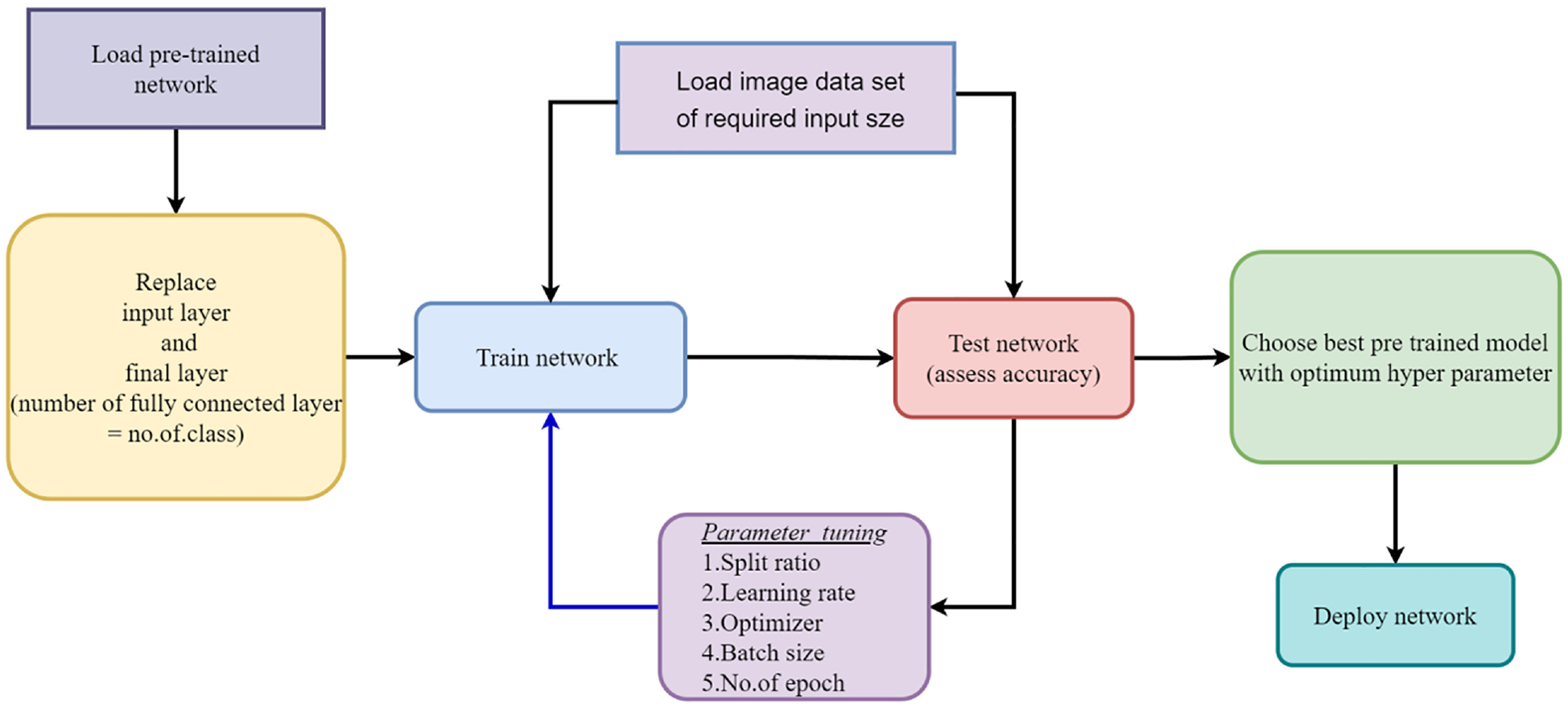
Workflow in using pre-trained networks.
Dataset preparation and pre-processing
In this study, spectrogram images generated from the vibration signals indicating suspension component faults are utilized. This technique offers a comprehensive representation of both time and frequency domain information within a signal. Converting the input signal into a spectrogram image allows the pre-trained network to capture details of both time and frequency information that may not be apparent in the raw data or spatial domain representation. Also, by representing data in the frequency domain, the model becomes less susceptible to noise and variations present in the time domain. Additionally, the process of converting the vibration signal into spectrogram images brings added advantages of dimensionality reduction. Consequently, this process significantly enhances the model’s performance in fault detection by enabling it to focus on the essential frequency components related to faults while disregarding transient noise. This helps to reduce computational complexity and memory requirements, making the pre-trained network more efficient during both training and inference.
From the collected signals, a dataset consisting of spectrogram images depicting suspension system faults was created. This dataset encompassed eight distinct classes of images, specifically: LABJ, TRBJ, LABW, STMF, STED, LTP, STWO, and good condition. In total, 800 images were generated, with 100 images per class, utilizing the acquired vibration signals. To ensure compatibility with the chosen pretrained network employed in the study, the images were resized to dimensions of 224 × 224, 227 × 227, or 299 × 299. This resizing process aimed to harmonize the image sizes with the requirements of the pretrained network. Figure 7 showcases an illustration of the spectrogram images of different class considered in the study.
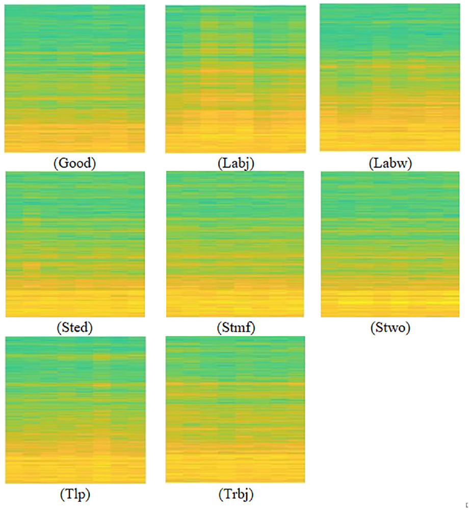
Spectrogram image for various suspension faults conditions.
AlexNet
The AlexNet pretrained network is an intricate convolutional neural network (CNN) composed of eight layers, initially devised for image classification tasks. It was introduced by Krizhevsky et al. in 2012 and emerged victorious in the ImageNet Large Scale Visual Recognition Challenge in the same year. 30 The architecture of AlexNet encompasses five convolutional layers and three fully connected layers. It employs a Rectified Linear Unit (ReLU) activation function and incorporates dropout regularization to mitigate the risk of over fitting. When provided with an input image of dimensions 227 × 227 × 3, the network produces a 1000-dimensional vector as output, which indicates the probabilities of the image belonging to each of the 1000 classes present in the ImageNet dataset.
GoogLeNet
The GoogLeNet pretrained network, commonly referred to as Inception-v1, is a sophisticated convolutional neural network developed by Google in 2014. It was introduced by Szegedy et al. and emerged triumphant in the ImageNet Large Scale Visual Recognition Challenge that same year. 31 The distinguishing feature of the GoogLeNet architecture lies in its utilization of Inception modules, which efficiently capture features at various spatial scales while minimizing the computational burden on the network. An Inception module comprises multiple parallel convolutional layers with different filter sizes and pooling operations, which are subsequently concatenated to create a comprehensive, multi-scale feature representation. The network also incorporates global average pooling to reduce the number of parameters and prevent over fitting. When provided with an input image of dimensions 224 × 224 × 3, the GoogLeNet pretrained network produces a 1000-dimensional vector as output, indicating the probabilities of the image belonging to each of the 1000 classes encompassed in the ImageNet dataset.
ResNet 50
ResNet, short for Residual Neural Network, is an advanced deep neural network that was meticulously crafted by Microsoft Research in 2015. 32 It falls under the category of convolutional neural networks (CNNs) and stands out due to its inclusion of residual blocks, which effectively address the vanishing gradient problem and enable the construction of significantly deeper neural networks. ResNet has gained substantial popularity as a pre-trained network architecture extensively employed in a multitude of computer vision tasks. With an impressive 152 layers, it has achieved remarkable performance on esteemed benchmark datasets, including ImageNet. The ResNet architecture encompasses multiple residual blocks, wherein the input signal traverses through a convolutional layer, followed by a batch normalization layer and an activation function. This output is then combined with the previous layer’s output, ensuring the preservation and utilization of essential information throughout the network’s depth.
ResNet101
ResNet-101, an extension of the original ResNet network, is a deep convolutional neural network architecture renowned for its exceptional performance across diverse computer vision tasks. Its introduction by He et al. in 2015 marked a significant milestone. 32 The “101” in its name signifies the impressive depth of the network, boasting a staggering total of 101 layers. The defining characteristic of ResNet-101 lies in its incorporation of residual blocks, which serve as fundamental building blocks within the architecture. These blocks encompass multiple convolutional layers, along with essential components like batch normalization and non-linear activation functions such as ReLU. The pivotal innovation of ResNet-101 lies in the introduction of residual connections also referred to as skip connections. These connections facilitate the learning of residual mappings within the network. By allowing the flow of gradients to circumvent layers, these connections effectively address the challenge of vanishing gradients encountered in deep networks. ResNet-101 capitalizes on these residual connections to capture and comprehend residual information, which signifies the disparity between the desired output and the input at each layer. By propagating this residual information, the network adeptly trains deeper architectures without experiencing performance degradation.
VGG-16
The VGG-16 pretrained network, an intricate deep convolutional neural network, was crafted by the esteemed Visual Geometry Group at the University of Oxford. Introduced by Simonyan and Zisserman in 2014, it achieved remarkable accuracy in the renowned ImageNet Large Scale Visual Recognition Challenge. 33 The VGG-16 architecture comprises 13 convolutional layers and three fully connected layers. Diverging from the approach of AlexNet, VGG-16 employs a compact 3 × 3 filter size across all convolutional layers, facilitating a deeper architecture while maintaining a relatively low parameter count. The network also incorporates the Rectified Linear Unit (ReLU) activation function and integrates dropout regularization techniques. Given an input image sized at 224 × 224 × 3, the VGG-16 network generates a 1000-dimensional vector as output, denoting the probabilities of the image belonging to each of the 1000 classes encompassed within the ImageNet dataset. The VGG-16 pretrained network has found widespread adoption as a foundational architecture for transfer learning in an array of computer vision tasks.
VGG-19
VGG19, similar to its predecessor VGG16, is a profound convolutional neural network that has made noteworthy contributions to the field of computer vision. Developed by the distinguished Visual Geometry Group at the University of Oxford, VGG19 elevates the VGG16 architecture to new heights with a total of 19 layers. Introduced by Simonyan and Zisserman in 2014, VGG19 attained commendable accuracy in the esteemed ImageNet Large Scale Visual Recognition Challenge. The architecture of VGG19 comprises 16 convolutional layers, complemented by three fully connected layers. Just like VGG16, VGG19 embraces the utilization of a compact 3 × 3 filter size in all convolutional layers, affording the network greater depth while maintaining a commendably restrained parameter count. VGG19 employs the rectified linear unit (ReLU) activation function and integrates dropout regularization, augmenting the network’s capacity to acquire knowledge and generalize effectively. In typical usage scenarios, VGG19 expects an input image size of 224 × 224 × 3 and produces a 1000-dimensional vector as output, denoting the probabilities of the image belonging to each of the 1000 classes encompassed within the ImageNet dataset. By employing smaller filters, VGG19 adeptly captures intricate details and learns discerning features across diverse object categories. Consequently, VGG19 has emerged as an invaluable tool in numerous tasks, including image classification, object detection, and semantic segmentation.
Mobilenetv2
MobileNetV2, exquisite convolutional neural network architecture, has garnered notable acclaim in the area of computer vision applications, particularly in environments constrained by resources, such as mobile and embedded devices. It was developed by the team in Google, strives to strike a delicate balance between model size, computational efficiency, and exceptional accuracy. MobileNetV2 presents a lightweight yet formidable solution for an array of computer vision tasks. At its core, MobileNetV2 places great emphasis on efficiency as a defining characteristic. It achieves this by employing depth wise separable convolutions, which disassemble the conventional convolutional operation into distinct depth wise and point wise convolutions. This clever approach effectively diminishes the computational burden by reducing the number of parameters and overall model complexity. Through the integration of this efficient convolutional operation, MobileNetV2 triumphs in attaining remarkable accuracy while preserving a compact model size. Such qualities render it remarkably suitable for seamless deployment on devices with limited resources.
Densenet201
DenseNet-201, a remarkable deep convolutional neural network architecture, has garnered attention for its exceptional performance in computer vision tasks. Introduced by Huang et al. 34 in 2017, DenseNet-201 represents a significant advancement in feature learning and representation capabilities. A distinguishing feature of DenseNet-201 lies in its dense connectivity pattern. Where, direct connections are established between all layers, forming a densely connected block. This dense connectivity facilitates seamless information flow and gradient propagation, fostering the development of more discriminative and expressive representations. Notably, DenseNet-201 effectively addresses the vanishing gradient problem by incorporating short paths between layers, ensuring efficient gradient propagation. This architectural innovation not only eases the optimization process also, improve the network to tackle the degradation issues typically associated with deep models. Overall, DenseNet-201 presents a powerful solution that enhances feature learning, gradient propagation, and network optimization, leading to superior performance in various computer vision tasks.
ShuffleNet
ShuffleNet, a convolutional neural network introduced by Zhang et al. 35 in 2018, presents a ground breaking approach to reduce computation complexity while preserving competitive levels of accuracy. One remarkable feature of ShuffleNet lies in its utilization of channel shuffling. By rearranging feature maps across channels, ShuffleNet enhances information flow and fosters cross-channel interactions, effectively augmenting the network representational capacity. This shuffling operation brings about a significant reduction in computational costs when compared to conventional convolutional neural networks, rendering ShuffleNet exceptionally efficient for resource-constrained environments. The boost in efficiency is accomplished through a combination of point wise group convolutions and depth wise separable convolutions. These operations minimize the number of parameters and computational requirements while retaining the ability to capture intricate features and patterns. By striking a balance between model size and accuracy, ShuffleNet presents a splendid solution for deployment on devices with limited resources.
Inception v3
Inception V3, a profound convolutional neural network architecture introduced by Szegedy et al. in 2015, has revolutionized the field of computer vision. Renowned for its remarkable performance in image classification tasks, Inception V3 has become a widely adopted model for diverse computer vision applications. One key element of Inception V3 is its distinctive inception module. This module incorporates parallel convolutional branches with varying filter sizes, enabling the network to capture both local and global features across different scales. This multi-scale approach empowers Inception V3 to extract diverse and discriminative features from input images, resulting in unparalleled classification accuracy.
Inception V3 also integrates auxiliary classifiers strategically positioned within the network to address the vanishing gradient problem during training. By incorporating these auxiliary classifiers, Inception V3 facilitates the propagation of gradients through different paths, ensuring more effective and stable gradient flow during backpropagation. Furthermore, Inception V3 leverages advanced architectural techniques like batch normalization and factorized convolution. Batch normalization plays a crucial role in reducing internal covariate shift, stabilizing the training process, and enhancing generalization. On the other hand, factorized convolution reduces computational costs by decomposing standard convolutions into smaller operations, reducing both the number of parameters and the overall complexity of the model. These architectural enhancements collectively contribute to the superior classification accuracy achieved by Inception V3.
InceptionresnetV2
Inception-ResNet-v2, an advanced convolutional neural network architecture introduced by Szegedy et al. in 2016, represents a powerful fusion of the Inception module and ResNet. This hybrid model has garnered remarkable achievements across diverse computer vision tasks, including image classification, object detection, and semantic segmentation. A key innovation of Inception-ResNet-v2 lays in its integration of residual connections within the inception modules. These connections facilitate efficient gradient flow, mitigating the challenges posed by the vanishing gradient problem and enabling smoother training of deep networks. By combining the multi-scale feature extraction capability of the Inception module with the skip connections of ResNet, Inception-ResNet-v2 enhances both representation capacity and optimization efficiency. Inception-ResNet-v2 also employs other cutting-edge architectural techniques such as batch normalization and factorized convolutions. These techniques contribute to improved training stability, faster convergence, and reduced computational complexity. Additionally, the incorporation of bottleneck layers further enhances efficiency by reducing the number of parameters and computational requirements.
Xception
Xception, a deep convolutional neural network architecture introduced by François Chollet in 2016, stands as a remarkable innovation in image classification and computer vision tasks. The term “Xception” derives from “Extreme Inception,” signifying its heightened version of the Inception module. Xception pushes the boundaries by incorporating depth wise separable convolutions. The key breakthrough of Xception lies in its utilization of depth wise separable convolutions, effectively dividing the conventional convolution operation into separate depth-wise and point-wise convolutions. This pioneering approach significantly reduces computational complexity and parameter count while preserving the extraction of meaningful features. By decoupling spatial and cross-channel filtering, Xception achieves superior efficiency and offers a computationally lightweight alternative to traditional convolutional neural networks. Table 4 summarize the characteristic features of chosen pre-trained network.
Characteristic features of pre-trained networks.

Results and discussion
In this current study, the performance of the well-established 12 pre-trained networks such as such as AlexNet, GoogLeNet, VGG-16, VGG19, ResNet-50, ResNet101, DenseNet201, MobileNetV2, InceptionV3, InceptionResNetV2, Xception, and ShuffleNet for suspension system fault diagnosis is evaluated. The experiment conducted by varying four hypermeters. They are Split ratio, solver (optimizer), Learning rate, and batch size. The experiments were conducted using the deep learning toolbox application in the MatLab 2019B software. The detailed experimental study is explained as follows.
Effect of train-test split ratio
In the current study, the dataset consisting of 100 images for each fault condition was divided into two parts: training data and testing data. Typically, the training data is allocated to be more than 60% of the given dataset, while the remaining portion is used to evaluate the performance of the trained model. To ensure consistent evaluation, we experimented with five different train-test split ratios. During these experiments, the parameters such as solver, batch size, and learning rate were kept constant. Specifically, we used sgdm as the solver, while the batch size and learning rate were set to 10 and 0.0001, respectively. Table 5 provides an overview of the performance of various pre-trained networks for different train-test split ratios. Inside the brackets in Table 5, one can find the shortest training time for each pre-trained network, along with the corresponding maximum classification accuracy.
Performance of pre-trained network for different train-test split ratio.

The minimum time taken to train the model with maximum accuracy is indicated within the brackets.
From Table 5, one can observe that the performance of the pre-trained networks varies depending on the chosen train-test split ratio. It is evident from the table that most of the pre-trained networks achieve the highest accuracy when the split ratio is set to 0.85, except for vgg16 and VGG19 networks. For the given dataset, VGG16 and vGG19 networks achieve the maximum classification accuracy at split ratios of 0.8 and 0.75, respectively. Therefore, for further parameter tuning, the split ratio that corresponds to the highest classification accuracy with the least training time for the model is used. Additionally, it is worth noting that among all the pre-trained networks, AlexNet requires the least amount of time to train the models.
Effect of solver
Solvers (optimizers) are the algorithms utilized to fine-tune the parameters, including weights and biases, of a neural network. The primary goal of these algorithms is to optimize the network’s performance by minimizing the loss value during the training process. In this particular study, systematic approach to explore the effectiveness of different optimizers, namely Root Mean Square Propagation (RMSprop), Stochastic Gradient Descent (SGDM), and Adaptive Moment Estimation (Adam), was used to evaluate the model performance. To maintain consistency in the experimentation, several parameters are kept unchanged, including the learning rate, batch size, and epoch values. Specifically, the values are set to 0.0001, 10, and 10 for learning rate, batch size, and epoch respectively. Additionally, the train-test split ratio was determined based on a previous experiment that yielded the highest accuracy for the specific network configuration. The outcomes of the pretrained network for each optimizer variation were recorded and are presented in Table 6. Notably, from the Table 6, it is evident that, apart from ShuffleNet, all other networks exhibited commendable performance when paired with the SGDM optimizer. This particular combination resulted in the highest classification accuracy while requiring less training time. Hence for further parameter tuning Sgdm is used as optimizer except ShuffleNet.
Performance of pre-trained network for various solvers.
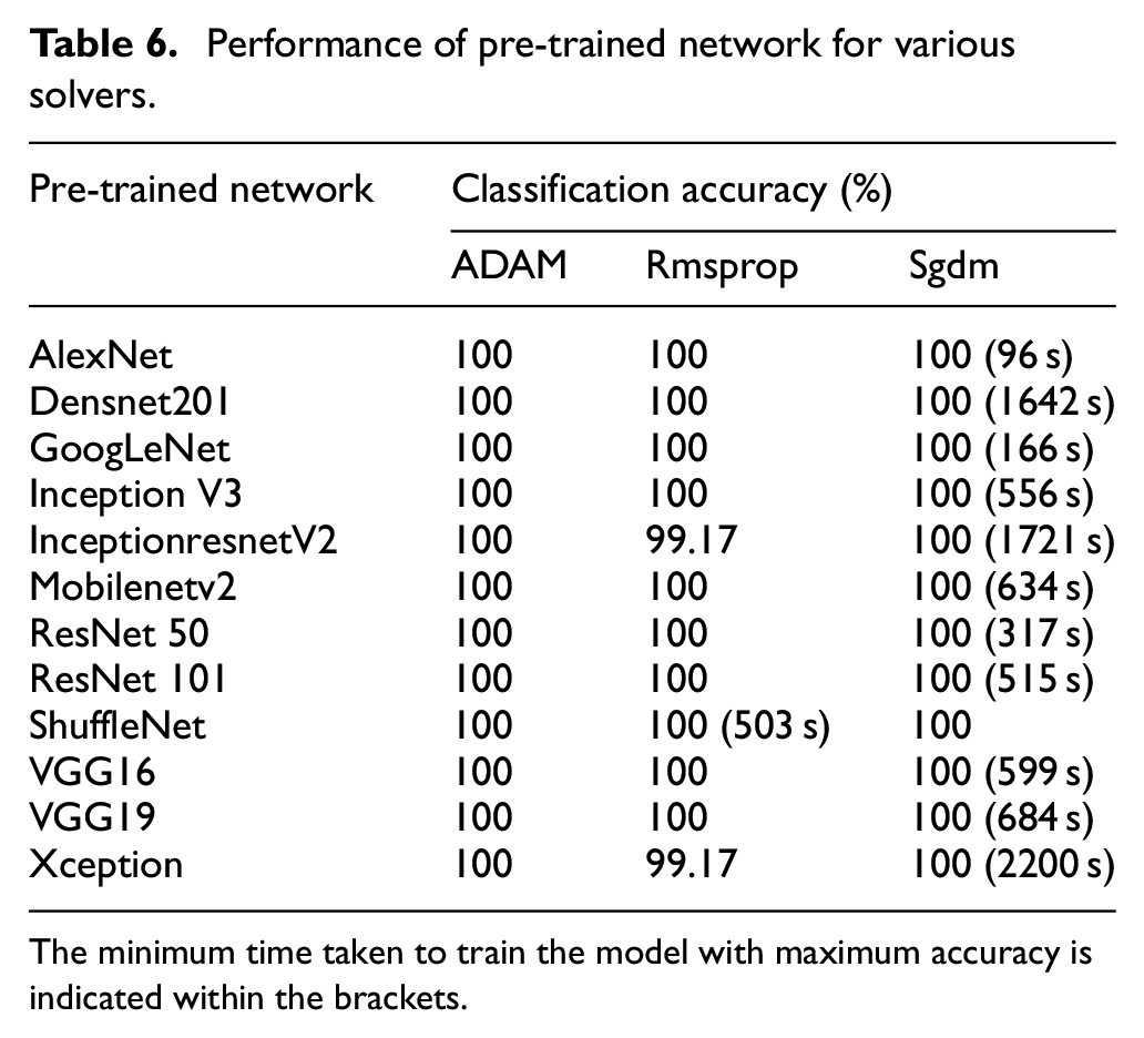
The minimum time taken to train the model with maximum accuracy is indicated within the brackets.
Effect of learning rate
The learning rate serves as a crucial hyper parameter that governs the rate at which model parameters, such as weights and biases, are updated during the training process. Selecting an appropriate learning rate is vital to achieve optimal model performance. If the learning rate is set too high, the model learns quickly. However, may overlook important nuances in the data. Conversely, a low learning rate prolongs computational time. In this study, the performance of the pre trained model was evaluated for different learning rates: 0.001, 0.0001, and 0.0003. During this evaluation, the parameters for the pretrained networks, including the train-test ratio and optimizer, were fixed based on the results of previous experiments. Additionally, the default values for batch size and epoch were maintained. Table 7 presents the performance of the pretrained models for the varying learning rates, considering the tuned values of the train-test split ratio and optimizer, along with the default batch size and epoch.
Performance of pre-trained network for different learning rates.
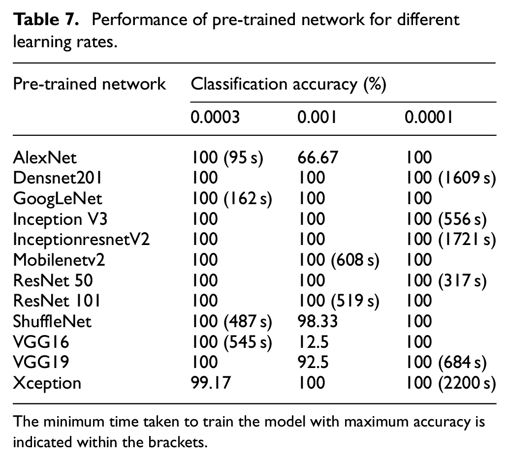
The minimum time taken to train the model with maximum accuracy is indicated within the brackets.
By examining Table 7, it becomes evident that the majority of pretrained networks considered, achieves optimal classification accuracy and minimizes training time when the learning rate is set to 0.0001. Notably, networks such as AlexNet, GoogLeNet, ShuffleNet, and VGG16 demonstrate maximum accuracy when the learning rate is adjusted to 0.0003. On the other hand, MobileNet V2 and ResNet 101 exhibit strong performance when the learning rate is set to its maximum value of 0.001.
Effect of batch size
Batch size refers to the number of samples processed in a training network before updating the model’s weights. The choice of batch size is a critical factor as it directly impacts training time and memory consumption. A larger batch size accelerates training by processing more samples in each iteration However, it requires more memory resources. Conversely, a smaller batch size lengthens the training process. Thus, it is crucial to optimize the batch size for a specific model. In the present study, we evaluated four different batch sizes (10, 16, 24, and 32) while considering the best-performing hyperparameters determined from the experimental results mentioned in previous sections. The value of remaining hyperparameter epoch is kept fixed based on previous experiment, Table 8 showcase the performance of pretrained models for each batch size, shedding light on their respective outcomes.
Performance of pre-trained network for different batch size.

The minimum time taken to train the model with maximum accuracy is indicated within the brackets.
Effect of epoch
An epoch represents a complete iteration of the training dataset being processed by the model. During training, the dataset is divided into smaller batches, and after each batch is processed, the model updates its weights and biases using an optimizer and calculates the loss. Once all the batches have been processed, one epoch is completed. The duration required to minimize the losses depends on the complexity of the pretrained network and its initial parameter values. Selecting an appropriate epoch value is essential to achieve optimal model performance. If the epoch value is set too low, the model may fail to capture intricate patterns, leading to under fitting. Conversely, if the epoch value is excessively high, the model may over fit to the specific dataset, losing its ability to generalize to new data. Additionally, a higher epoch value prolongs the training time. Hence, determining the optimal number of epochs for each pretrained model is crucial for a given dataset. In the present study, epoch values of 10, 20, and 30 were considered, and the corresponding performance of the pretrained networks for these values was recorded and is presented in Table 9.
Performance of pre-trained network for different epoch.
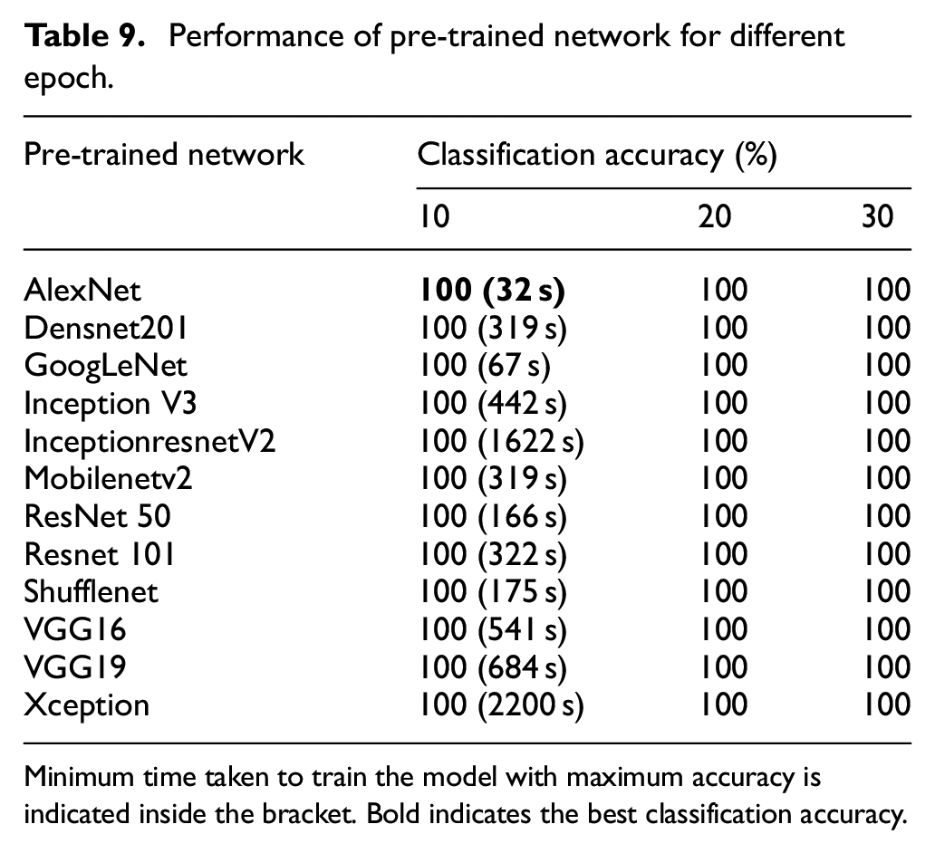
Minimum time taken to train the model with maximum accuracy is indicated inside the bracket. Bold indicates the best classification accuracy.
Performance comparison of pre-trained models
From the experimental results conducted earlier, the multiple hyper parameters values that optimize the performance of the pre-trained models were identified. The hyper parameters that maximize the model performance are provided in Table 10. The output for the tuned hyper parameter of the pretrained network was presented in Table 11 performance of pre-trained networks with chosen hyper parameters are depicted.
Optimal hyper parameters for pre-trained network.

Bold indicates the optimal hyperparameter setting.
Performance of pre-trained network for optimum hyper parameter value.

Analyzing Table 11 reveals that, among the 12 networks, AlexNet demonstrates the highest accuracy, achieving this feat with a minimal training time of 32 s. Following closely, GoogLeNet and ResNet50 exhibit maximum classification accuracy, accomplishing efficient model training within 67 and 166 s, respectively. Figure 8 visually charts the training progress of the AlexNet model, while Figure 9 presents the corresponding loss plot of AlexNet model. Furthermore, the proposed AlexNet pretrained model, configured with a 0.85 split ratio, Sgdm optimizer, a learning rate of 0.0003, a batch size of 32 and 10 epochs effectively classifies faults using spectrogram images generated from vibration signals. This approach was tested on signals acquired from the experimental setup showcasing its applicability in real-time conditions. To maximize the potential of machine learning and deep learning in real-world scenarios frequent model updates tailored to the environment and road conditions are essential. In this context, the proposed pretrained model with its capability for automated feature engineering and reduced computational resource requirements proves advantageous in dynamic real-time conditions.

Training process of AlexNet network with optimal hyper parameter.
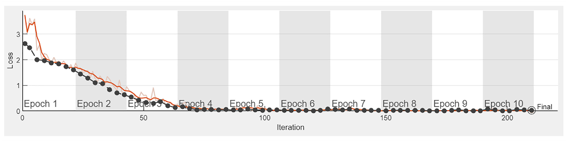
Loss plot of AlexNet network with optimal hyper parameter.
The training progress is depicted in Figure 8, indicating that the training process attained saturation after the fifth epoch. This saturation indicates that the AlexNet network has been effectively trained on the given suspension system dataset. The confusion matrices demonstrate the performance of a specific model or algorithm at the class level as shown in Figure 10. The diagonal elements of the matrices represent correctly classified instances, while the adjacent elements to the diagonal indicate misclassifications within their corresponding classes. From Figure 10, the confusion matrix of the AlexNet model reveals that the trained model can classify suspension component faults with 100% accuracy. It can be observed that all 15 test samples from each class were classified correctly. Therefore, it is recommended to use the model built with AlexNet for diagnosing faults in suspension systems using spectrogram images, as it shows promising results for the given dataset.

AlexNet network Confusion matrix.
Conclusion
This paper investigates the use of 12 pre-trained deep learning models to diagnose faults in suspension systems by utilizing spectrogram images derived from acquired vibration signals. The study specifically focuses on seven fault conditions: worn-out lower arm ball joint, worn-out tie rod ball joint, worn-out lower arm bush, strut mount failure, external strut damage, worn-out strut, and low tire pressure. A reference image representing a good condition is also included. These pre-trained networks are equipped with convolutional neural network (CNN) layers, which employ a hybrid approach encompassing feature extraction, feature selection, and fault classification. This forms an end-to-end deep learning framework. The results demonstrate that these pre-trained networks effectively process spectrogram images and yield highly accurate classification results. By carefully adjusting various hyperparameters such as learning rate, batch size, epoch, train-test split ratio, and optimizer, optimal settings were identified for all the networks. Comparative studies revealed that among the considered networks, AlexNet exhibited superior performance. It demonstrated efficient training, requiring minimal time, while achieving a fault classification accuracy of 100%. Therefore, for real-time applications involving fault diagnosis in suspension systems using spectrogram images from vibration signals, this study recommends the utilization of AlexNet due to its exceptional performance and accuracy.
Footnotes
Handling Editor: Sharmili Pandian
Declaration of conflicting interests
The author(s) declared no potential conflicts of interest with respect to the research, authorship, and/or publication of this article.
Funding
The author(s) received no financial support for the research, authorship, and/or publication of this article.
Data availability
The data used to support the findings of this study are included within the article and further data or information can be obtained from the corresponding author upon request.