Sage Journals: Discover world-class research

Abstract

TBM tunnel surrounding rock classification is a key indicator for supporting decision-making and ensuring safe construction. And predicting the surrounding rock type accurately in advance is of great significance for TBM intelligent construction. This paper established the surrounding rock classification model based on support vector machine (LIBSVM), including preprocesses historical tunneling parameters, extracts data information that can accurately reflect the relationship between rock and machine, analyzes the correlation between different parameters and surrounding rock categories, and obtains highly relevant parameters. Based on the long short-term memory (LSTM), the prediction model of total thrust, cutter head torque, gripper pressure, cutter head rotate speed, and propulsion speed are established, which is the strongly correlated parameters with surrounding rock. Combining the parameter prediction model with the surrounding rock classification algorithm, the LSTM-SVM tunnel surrounding rock classification prediction model is established. The results showed that the coefficient of determination of the total thrust model, the cutter head torque, the gripper pressure, the cutter head speed, and the propulsion speed were 0.9825, 0.9396, 0.9974, 0.9843, and 0.9636. The overall prediction accuracy of the surrounding rock category can reach 86.0686%, which can provide a certain reference for predicting the surrounding rock condition in a short distance.

Keywords

Tunneling parameters surrounding rock classification LSTM-SVM surrounding rock class prediction TBM

Introduction

TBM is a kind of large-scale digital tunneling equipment, which is widely used in subways, water conservancy, highways, railways tunnel construction.^1–3 In the process of TBM construction, the type of surrounding rock is the key index of surrounding rock stability evaluation and tunneling performance prediction.^4,5 Predicting the surrounding rock classes accurately within a short distance is very helpful for the workers to formulate corresponding supporting measures in time. Moreover, the workers can conduct operation adjustment and preparation in time according to the judgment of geological conditions ahead. Therefore, it is of great significance to improve the TBM construction safety and effectiveness.

The traditional tunnel surrounding rock class is based on the data obtained from the current rock mass property test or various parameters through calculation, which cannot be directly predicted. At present, in terms of the research on the prediction of related properties of surrounding rocks of TBM tunnel at home and abroad, Liu et al. established an empirical model for TBM performance prediction of hard rock based on HC multiple regression analysis. According to the engineering data of different tunnels.^6,7 Jamshidi established regression analysis prediction model of TBM cutting depth and surrounding rock brittleness index by using multiple regression analysis.⁸ Yagiz et al. respectively adopted intelligent methods such as fuzzy recognition, neural network, and particle swarm optimization to establish the prediction model of TBM excavation rate and rock brittleness index.⁹ Qiu et al. proposed an advanced classification method of surrounding rock class based on TSP203 system and genetic support vector machine.¹⁰ Gao et al. used three circulatory neural networks to predict TBM boring parameters.¹¹ Wang et al. combined with large number of tunneling data, obtained that the cutter head torque has a significant correlation with the surrounding rock class, cutter head speed, and propulsion speed. Based on this, the prediction model of cutter head torque NSVR was established.¹² Zheng et al. used particle swarm optimization algorithm to optimize the support vector machine algorithm, and established a prediction model of tunneling load based on operation parameters.¹³ Yu et al. has applied a novel semi-supervised method to establish the rock mass type prediction model ahead of the tunnel face.¹⁴ Xu et al. predicted TBM operational indicators using various statistical, ensemble, and deep neural network machine learning methods, and compared the merits and demerits between different method.¹⁵ Fu and Zhang put forward a spatio-temporal approach to forecast TBM’s penetration rate based on deep learning model.¹⁶ Wang et al. proposed a parameters prediction framework for TBM thrust, torque, and net advance rate based on machine learning method.¹⁷ Huo et al. established an advance prediction model of the rock mass category (RMC) with 99% prediction accuracy.¹⁸ Feng et al. introduced Field Penetration Index to quantify TBM performance using big data and deep learning.¹⁹ Kilic et al. used SMOTE method to identify TBM lithology through operational parameters, respectively.²⁰ And Heydari et al. investigated the relationship between various TBM operational factors.²¹

In conclusion, these researches mainly focus on the prediction of single rock mass indicator and tunneling load during TBM tunneling. While relatively few studies on the prediction of surrounding rock class. Traditional research of surrounding rock classification is based on the characteristics of rock mass, whose prediction accuracy and timeliness are poor as the difficulty in obtaining related indexes and limited samples. The TBM operational parameters of TBM during construction process are affected by the types of surrounding rocks, which are all strictly sequential over time. Therefore, it is a time-efficient and accurate method for surrounding rock classification through TBM operational parameters. In terms of the parameter prediction using engineering data, most studies are focused on the selection and optimization of operational parameters. There are few researches on TBM operational parameters and surrounding rock classification prediction. Most of sample sets are small and some data are experimental data rather than actual engineering data. While a large number of sample data are required for machine learning method to establish a more accurate prediction model. So, it may be feasible that predicting the type of surrounding rocks based on the predicted TBM operational parameters by means of machine learning method.

In this paper, combined with the historical excavation data of TBM, the statistical analysis is carried out to obtain the characteristic parameters. Based on the support vector machine algorithm in machine learning LIBSVM, the surrounding rock classification is realized. Then, based on the long-term and short-term memory network, the characteristic parameter prediction model is established, and combined with the surrounding rock classification algorithm, the LSTM-SVM short-distance surrounding rock class prediction model is established to realize the prediction of the surrounding rock class model of TBM tunnel in the tunneling process.

Methodology

The primary objective of the paper is to establish an intelligent prediction model for TBM tunnel surrounding rock classification based on the corresponding relationship between the operating parameters and rock classification. Figure 1 shows a flow chart of the prediction process formulated for the study. The process is divided into five steps: (1) collecting the original TBM data from TBM acquisition system for each tunnel ring, including all monitoring information during TBM operation. (2) Pre-processing the data to ensure clear and consistent results, including extracting the operating parameters in stable tunneling state, calculating the mean and variance of the data, and analyzing the correlation between data. (3) Establish the surrounding rock classification model according to TBM operating parameters sample set and rock mass class labels. (4) Establish the tunneling parameters prediction model based on the TBM operating parameters sample set. (5) Establish the surrounding rock class prediction model combing the surrounding rock classification model with tunneling parameters prediction model. Conducting five steps can achieve real-time prediction for the surrounding rock classification.

Figure 1.

Flow chart for prediction of TBM surrounding rock class

Establishment of the database

Geological conditions project overview

The data in this paper came from the main tunnel construction project with a total length of 19.87 km. An open TBM is used with excavated diameter of 7.0 m. The construction section of the project contains class II, class III, class IV, and class V surrounding rocks. The lithology of the surrounding rock is mainly tuff and tuff breccia, which are all hard rocks. The various surrounding rocks data provides a good data base for subsequent research. Based on the Basic Quality method, the exposed surrounding rocks of each ring are classified and matched with the tunneling parameters. The proportion of the collected surrounding rock class data is shown in Figure 2, where class II rock accounts for the largest proportion with 57.1%, and class IV takes up the minimum with 2.78%.

Figure 2.

Proportion of surrounding rock class data.

Engineering data preprocessing

The original data only the data collected in the stably advancing status can represent the interaction between rock and TBM machine. While the collected data in the abnormal tunneling conditions has a negative impact on the establishment of classification model. Therefore, in order to ensure the accuracy of the model training, the data filtration should be carried out before modeling, which including filtering data in non-tunneling status, filtering data in start-up and shut-down status, and filtering data in abnormal tunneling status.

(1) Filtering data in non-tunneling status

In the process of TBM construction, gripper change in step, surrounding rock support, cutter replacement, and machine maintenance all should be conducted with no advancement of TBM. Therefore, it is necessary to remove the data in these statuses, which is valueless for the analysis of the surrounding rock class. Then, filtering is carried out according to the binary discriminant function proposed by Wang et al.¹²

f (x) = {\begin{matrix} 1, (x > 0) \\ 0, (x \leq 0) \end{matrix}

(1)

D = f (F) \cdot f (v) \cdot f (T) \cdot f (n)

(2)

Status = {\begin{matrix} Normal, (D = 1) \\ Abnormal, (D = 0) \end{matrix}

(3)

Where, f is a binary discriminant function, D values in 0 or 1, $F$ is the total thrust of TBM, $v$ is the advance speed, $T$ is the torque of cutterhead, and $n$ is the rotate speed of cutterhead.

(2) Filtering data in start-up and shut-down status

The normal tunneling of TBM consists of start-up status, stable tunneling status, and shut-down status. Start-up and shut-down status contain acceleration and deceleration stages in each TBM operating cycle. These unstable data should be eliminated which may cause interference to the classification prediction of surrounding rocks. The data in start-up and shut-down status are culled according to the following rules: if the interval time between two breakpoints is less than 300 s, all data between two breakpoints are culled; if the interval between two breakpoints is more than 300 s, the data within 200 s after the start-up point and within 60 s before the stop point are eliminated. The curves of advance speed change with time a certain period before and after elimination processing is shown in Figure 3.

(3) Filtering data in abnormal tunneling status

Figure 3.

Diagram of propulsion velocity over time: (a) before filtering and (b) after filtering.

Filtering data in abnormal tunneling status is conducted according to the abnormal value of penetration. The penetration in normal tunneling status is mainly distributed between 0 and 32.7 mm/r. the penetration data is divided into groups according to the size, where the size distribution and cumulative percentage are shown in Figure 4.

Figure 4.

Distribution of penetration data.

It can be seen from Figure 4 that the average value in the tunneling status is 6.95 mm/r, which basically presents normal distribution. The data with penetration less than 13 mm/r account for over 97%, and the maximum penetration is 32.7 mm /r, which is obviously abnormal. Therefore, the data with penetration above 13 should be filtered.

Correlation analysis between operating parameters and surrounding rock classes

The data set recorded by TBM includes hundreds of types of data, many of which have no relation with TBM tunnel and geological parameters. These data should be excluded to reduce computation and improve accuracy of surrounding rock classification model. Therefore, it’s necessary to select the operating parameters closely related to the surrounding rock classes from the data set. So, the correlation direction and degree between different boring parameters and surrounding rock classes are discussed, and the parameters with high correlation are selected as data samples of the classification model.

The correlation coefficient is a quantity representing the degree of linear correlation between variables, which is represented by $r$ . The variation range of $r$ is [0, 1], where the value of $r$ and its corresponding correlation degree is shown in Table 1.

Table 1.

Variation range of correlation coefficient and its meaning.

Variation range of r	Correlation degree
<0.2	No linear correlation
0.2–0.4	Weak correlation
0.4–0.6	Moderate correlation
0.6–0.8	Strong correlation
0.8–1	Highly strong correlation

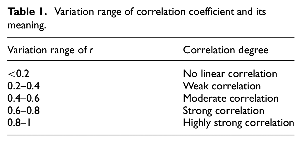
In this paper, Pearson correlation coefficient is selected to calculate the relationship between parameters and surrounding rock classes.

r = \frac{N \sum x_{i} y_{i} - \sum x_{i} \sum y_{i}}{\sqrt{N \sum {x_{i}}^{2} - {(\sum x_{i})}^{2}} \sqrt{N \sum {y_{i}}^{2} - {(\sum y_{i})}^{2}}}

(4)

Where, $x_{i}$ is the $i^{th}$ observation value of variable $X$ , and $y_{i}$ is the $i^{th}$ observation value of variable $Y$ .

The detailed characteristics of TBM operating parameters are analyzed based on Pearson correlation coefficient, and the correlation between TBM operating parameters and the surrounding rocks of Class II, III, IV, and V is obtained. The parameters above with strong correlation are shown in Table 2.

Table 2.

Correlation analysis between different parameters and surrounding rock classes.

TBM operating parameters	Correlation coefficient	Correlation degree
Gripper pressure	0.8085	Highly strong correlation
Propulsion speed	0.6250	Strong correlation
Total thrust	0.9075	Highly strong correlation
Cutter head speed	0.7850	Strong correlation
Cutter head torque	0.8843	Highly strong correlation

Surrounding rock classification model based on LIBSVM

Classifier selection

In order to realize the classification of surrounding rock more accurately, it is necessary to select the classifier with high performance. Firstly, the classifier needs to perform well in a certain number of training sets and avoid overfitting to the greatest extent. Secondly, the classifier should have the ability to classify samples in a non-linear manner when dealing with geological data in different alternate surrounding rock classes. SVM has strong generalization ability and high robustness, which is selected from many machine learning methods.^20–22 The LIBSVM is used to deal with multi-classification problems by means of voting. Its basic idea is to construct N(N−1)/2 class two classifiers out of N categories, and identify test samples using voting method. Compared with other multi-class support vector machine algorithms, LIBSVM has the advantages of fewer sub-classifiers and shorter training time.

Feature extraction and selection

Extracting and selecting appropriate feature parameters from the original parameters not only reduces the computational overhead, it also significantly improves the performance of the classifier, both of which are significant for an accurate identification of the surrounding rock class. In order to accurately reflect the condition of the surrounding rock, the time per revolution of the cutterhead is used as the time window. The cutterhead rotate speed range from 1 to 7.7 rpm, so the time window is set as 60 s, which is the lowest value of the rotation speed. It indicates that every 60 pieces of feature parameters in the time domain are taken as a sample to construct feature vector. Based on the analysis of the correlation and change rule of operating parameters and surrounding rock classes, feature vectors [x₁, x₂, x₃, x₄, x₅] is finally selected as the input vector for training and test, where denotes the average total propulsive force, the average cutter head torque, the average gripper pressure, the average cutter head rotation speed, and the average propulsion speed, respectively.

Surrounding rock class prediction model based on LSTM-SVM

LSTM method

TBM operating parameters change with time and are non-stationary time series. And because the output of traditional machine learning methods such as support vector regression or random forest is only determined by the current input without the help of previous learning information, they are also not suitable for real-time prediction of TBM tunneling parameters.¹¹ These traditional regressions models cannot act as real-time predictors in a practical sense, because they only reflect the mapping relationship between current parameters and input parameters, which is close to function fitting and cannot provide prediction values of operating parameters based on in situ data in the next period. In recent years, due to the rapid development of neural network, a variety of deep learning algorithms (such as recurrent neural network and convolution neural network) have been produced. Among them, recurrent neural network, namely RNN, can add a variety of gate operations to improve the training ability and efficiency. It is one of the most powerful tools to predict non-stationary time series, and the prediction effect is far better than the traditional machine learning method.

Recurrent neural network (RNN) has a cyclic structure, in which the previous output of hidden nodes is used to generate the response of the current input, so it is usually used to process the prediction task where the input samples are time series. Its source is to characterize the relationship between the current output of a sequence and the previous information. From the network structure, the recurrent neural network will remember the previous information and use the $t$ previous information to affect the output of the subsequent nodes. The nodes between the hidden layers are connected. The input of the hidden layer includes not only the output of the input layer, also includes the output of the hidden layer at the previous moment. Let ${\vec{h}}_{t} = {({h_{t}}^{(1)}, . . ., {h_{t}}^{(J)})}^{T}$ be the hidden output at time $t$ . Then, for the current input $x_{t + 1}$ , the output calculation formula of the $j^{th}$ hidden node is shown in (6):

\begin{matrix} h_{t + 1}^{(j)} = \tanh ((\sum_{i = 1}^{I} U^{(ji)} \cdot x_{t + 1}^{(i)}) + (\sum_{a = 1}^{I} U^{(ja)} \cdot h_{t}^{(a)})), \\ j = 1, 2, \dots, J . \end{matrix}

(5)

\tanh (x) = \frac{e^{x} - e^{- x}}{e^{x} + e^{- x}}

(6)

Where, $U^{(ji)}$ is the weight between the current input $x_{t + 1}^{(i)}$ and the hidden layer output $h_{t + 1}^{(j)}$ , and $W^{(ja)}$ is the weight between the current hidden output $h_{t + 1}^{(j)}$ and the previous hidden output $h_{t}^{(a)}$ . The output calculation formula of the $k^{th}$ fully connected node is shown in (7):

q_{t + 1}^{(k)} = \tanh (\sum_{k = 1}^{J} V^{(ki)} \cdot h_{t + 1}^{(j)}), k = 1, 2, \dots, K .

(7)

Where, $V^{(kj)}$ is the weight between the current hidden output $h_{t + 1}^{(j)}$ and the current output $q_{t + 1}^{(k)}$ . In general, Back Propagation Through Time (BPTT) algorithm is used to train the traditional RNN. But when the network is used for a long input sequence, because the gradient is always shrinking or increasing along the time back propagation, the training will be affected by gradient disappearance and gradient explosion. To improve the capabilities and training efficiency of traditional RNNs, gate operations can be imposed on hidden nodes, such as long short-term memory (LSTM) networks.

Long-term memory unit LSTM (Long Short-Term Memory)²³ combines three kinds of gate operations in its hidden node, including input gate, forget gate, and output gate, whose unit structure is shown in Figure 5. Its state is divided into two vectors: short-term state $h_{(t)}$ and long-term state $c_{(t)}$ . As the long-term state $c_{(t)}$ runs through the network from left to right, it first passes a forget threshold, discards some memories, and then adds some new memories through some additional operations. The output of $c_{(t)}$ is directly output without any operation. So, some memories are discarded and some memories are added at each time iteration. In addition, after additional operations, the long-term state is copied and passed into the tanh function, and then the result is filtered by the output threshold, so the short-term state $h_{(t)}$ is generated. And the working principle of the new memory is: first, the current input vector $x_{(t)}$ and the previous short-term state $h_{(t - 1)}$ are input to four different fully connected layers. The main layer is the layer whose output is $g_{(t)}$ . Its basic function is to analyze the current input $x_{(t)}$ and the previous short-term state $h_{(t - 1)}$ . However, there is only this layer in the basic unit, which directly outputs $y_{(t)}$ and $h_{(t)}$ . In contrast, LSTM units do not output directly, but store part of the output in a long-term state. The other three layers are threshold controllers, whose output ranges from 0 to 1 by using of logical activation functions. As shown in the Figure 5, their output is input into the element intelligent multiplication operation. So if the output is 0, then the threshold is closed; if the output is 1, then the threshold is opened. In particular, forget threshold (controlled by $f_{(t)}$ ) determines which long-term states should be discarded; input threshold (controlled by $i_{(t)}$ ) determines which parts of $g_{(t)}$ will be added to the long-term state; output threshold (controlled by $o_{(t)}$ ) determines which long-term states should be read and output ( $h_{(t)}$ and $y_{(t)}$ ) at this time iteration.

Figure 5.

Basic cell structure of LSTM.

Formulas (8–13) summarize how to calculate the long term state, short term state, and output of a unit in a single instance at each time iteration.

i_{(t)} = σ (W_{xi}^{T} \cdot x_{(t)} + W_{hi}^{T} \cdot h_{(t - 1)} + b_{i})

(8)

f_{(t)} = σ (W_{xf}^{T} \cdot x_{(t)} + W_{hf}^{T} \cdot h_{(t - 1)} + b_{f})

(9)

o_{(t)} = σ (W_{xo}^{T} \cdot x_{(t)} + W_{ho}^{T} \cdot h_{(t - 1)} + b_{o})

(10)

g_{(t)} = \tanh (W_{xg}^{T} \cdot x_{(t)} + W_{hg}^{T} \cdot h_{(t - 1)} + b_{g})

(11)

c_{(t)} = f_{(t)} \otimes c_{(t - 1)} + i_{(t)} \otimes g_{(t)}

(12)

y_{(t)} = h_{(t)} 2 = o_{(t)} \otimes \tanh (c_{(t)})

(13)

Where, $W_{xi}$ , $W_{xf}$ , $W_{xo}$ , $W_{xg}$ are the weight matrix of each layer connected to the input vector $x_{(t)}$ ; $W_{hi}$ , $W_{hf}$ , $W_{ho}$ , $W_{hg}$ are the weights matrix of each layer connected to the previous short-term state $h_{(t - 1)}$ ; $b_{i}$ , $b_{f}$ , $b_{o}$ , $b_{g}$ are the deviation coefficients of each layer.

Data preprocessing and model evaluation indexes

By performing feature extraction on the original tunneling data of each parameter, the new sample sequence is established as 38,400. Then, the sequence is divided into two time-continuous subsequences: the first 90% and the last 10%. The former is used to train the prediction model and the latter is used as a test set. Secondly, in order to improve the prediction accuracy, reduce the training time of the model, and avoid the influence of the different dimensions of each data on the LSTM network model, the Z-score method is used to standardize the data vector based on the time series data of tunneling parameters. The input data vector is normalized to a standardized sequence with a mean of 0 and a standard deviation of 1. The standardized expression as shown in (14):

x_{n} = \frac{x_{i} - μ}{σ}

(14)

Where, $x_{n}$ represents the standardized data in training set and test set, $x_{i}$ represents the original data in test set and training set, μ is the mean of all sample data, and σ is the standard deviation of all sample data.

Regression (prediction) model has many evaluation indexes, which can directly reflect the accuracy of prediction results. Based on the research of a large number of time series prediction, Root Mean Square Error (RMSE), Mean Absolute Percentage Error (MAPE), and Coefficient of Determination (R²) are chosen as the evaluation indexes of the accuracy of prediction results.

(1) Root Mean Square Error:

RMSE = \sqrt{\frac{\sum_{i = 1}^{N} {(y_{i} - {\tilde{y}}_{i})}^{2}}{N}}

(15)

(2) Mean Absolute Percentage Error:

M A P E = \frac{1}{N} \sum_{i = 1}^{N} | \frac{y_{i} - {\tilde{y}}_{i}}{y_{i}} | \times 100 %

(16)

(3) Coefficient of Determination:

R^{2} = 1 - \frac{\sum_{i = 1}^{N} {(y_{i} - {\tilde{y}}_{i})}^{2}}{\sum_{i = 1}^{N} {(y_{i} - \bar{y})}^{2}}

(17)

Where, N represents the number of prediction samples, $y_{i}$ , ${\tilde{y}}_{i}$ , and $\bar{y}$ represent the real value, prediction value, and average of real value of various parameters. Among the three evaluation indexes, the model with larger $R^{2}$ is preferred, followed by the model with smaller MAPE and RMSE.

Prediction model of operating parameters

Predicting the five TBM tunneling parameters should be conducted before establishing the surrounding rock prediction model. Parameter prediction model based on LSTM network includes: input layer, LSTM layer with 288 nodes, fully connected layer and output layer with 1 node (logistic regression layer). The network uses the Adam optimization algorithm to optimize the loss function, which is different from the stochastic gradient descent algorithm (SGD) used in the traditional BP neural network. It combines the characteristics of adaptive optimization algorithm (AdaGrad) that is sensitive to sparse matrix information and RMSprop algorithm that has good convergence to the unstable objective function, while adding a momentum term to avoid the search direction swings, speed up the convergence. Adam optimization algorithm also has the advantages of simple adjustment of super parameters such as learning rate and suitable for large-scale data and application. In the network model, the number of iterations, the gradient threshold, and the initial learning rate is set as 250, 1, and 0.005, respectively. Moreover, the learning rate decline cycle and decline factor is set as 125 and 0.2 respectively. The whole process of training is shown in Figure 6.

Figure 6.

LSTM network flowchart for parameter prediction.

Before establishing the prediction model, it is necessary to transform the data of the training set. The historical operating parameters of a certain time step is taken as the input variables, and the parameter value of the next time step is taken as the output variables. It indicates that the previous boring parameter data ${x_{t - τ + 1}, x_{t - τ + 2}, . . ., x_{t - 1}, x_{t}}$ is used to predict the next time $x_{t + 1}$ data. This method is called sliding window method, where the number of steps in the past time is called window width $τ$ . The width of the sliding window is the basis of prediction model. The five characteristic parameters total thrust, cutterhead torque, shoe support pressure, cutterhead rotate speed, and advance speed are expressed as x⁽¹⁾, x⁽²⁾, x⁽³⁾, x⁽⁴⁾, x⁽⁵⁾, respectively. Taking the total thrust x⁽¹⁾ as an example, when the sequence is ${x_{1}^{(1)}, x_{2}^{(1)}, \dots, x_{34560}^{(1)}}$ , assume the training window width τ = 5, and the training samples for the LSTM network predictor f are formed as follows:

\begin{matrix} ({x_{1}^{(1)}, x_{2}^{(1)}, \dots, x_{5}^{(1)}}, x_{6}^{(1)}); \\ ({x_{2}^{(1)}, x_{3}^{(1)}, \dots, x_{6}^{(1)}}, x_{7}^{(1)}); \\ ⋮ \\ ({x_{34555}^{(1)}, x_{34556}^{(1)}, \dots, x_{34559}^{(1)}}, x_{34560}^{(1)}) \end{matrix}

(18)

It means that when a time-continuous sequence of five operating parameter data are input to the trained LSTM-based predictor f, the five operating parameter value in the next time $f (x_{t - 4}, x_{t - 3}, \dots, x_{t - 1}, x_{t}) = {\hat{x}}_{t + 1}^{(1)}$ can be generated. And the optimal window width is different for different training objects. In general, the larger the input window width is, the more information it contains and the higher the prediction accuracy is. But the data used for training and prediction in this paper is the TBM operating parameters which are strongly related to the surrounding rock properties. It has certain non-replication on the natural geological distribution. The historical data that far away from the real-time tunneling point may be greatly different from the data under the current surrounding rock condition, even negatively affecting the accuracy of prediction. So, when establishing a five-parameter prediction model, the influence of different window widths on the prediction accuracy of the model should be analyzed separately, and the optimal number of input parameters should be selected to improve the prediction accuracy.

Experiment results

Establishment of the database

Because the surrounding rock classification model takes every 60 data in the time domain as a sample and its mean value or standard deviation is taken as the feature for recognition, the direct prediction of 60 data in the next minute cannot reflect the characteristics of the sample well, which will increase the error of prediction result. To solve this problem, the characteristics of each sample should be predicted directly. First of all, preprocess the data, take every 60 s as a sample, extract its mean value and other features, and re-establish the sample set for training and testing. Taking the total thrust as an example, Figure 7 is the original effective thrust data, and Figure 8 is the new sample set established after feature extraction. It can be seen from figures that the sample set after feature extraction can reflect the change rule of total thrust with time, without changing its characteristics in time domain. Therefore, the new sample set can also reflect the change rule of surrounding rock class. It’s effectively to improve the prediction accuracy of surrounding rock class by using the feature values of operating parameters to directly identify the feature values of the next stage.

Figure 7.

Original boring data of total thrust.

Figure 8.

Total thrust boring data after feature extraction.

Training based on LIBSVM model

Four thousand sets of feature vectors [x₁, x₂, x₃, x₄, x₅] of different surrounding rock classes are extracted from the original operating parameters, where each class have 1000 sets. The values 1, 2, 3, and 4 are used to define the output of the four classes of surrounding rocks: II, III, IV, and V, respectively. In order to uniform the variation range of each feature value in the feature vector, all feature values are normalized and linearly transformed into [−1, +1]. Then, 4000 sets of feature vectors and corresponding surrounding rock classes construct the sample set. According to the recommended ratio widely used in machine learning research, the sample set is randomly divided into two groups with a ratio of 6:4.

The LIBSVM model is used to train and test the sample set. According to the design experience and recognition results, the radial basis function is selected as the kernel function of LIBSVM. In addition, the kernel function parameters γ and penalty coefficient $c$ in the array of [2⁻¹⁰, 2^−9.5, 2⁻⁹, …, 2⁹, 2^9.5, 2¹⁰] are selected to train the model respectively. A 10-fold cross-validation is conducted by continuously adjusting the model parameters (support vectors and relaxation variables) to ensure the optimal classification performance of the model. Figure 9 shows the cross-validation results of LIBSVM with different hyperparameters. The areas with high accuracy are concentrated in the lower right corner, where γ takes [4, −10], c takes [−4, 10]. When the kernel parameter and penalty coefficient are 0.1768 and 5.6569 respectively, the recognition accuracy of cross-validation results using training sets is up to 100%. High penalty parameters can improve the accuracy of the training set, but will lead to the over-learning state and cannot obtain ideal test result. Therefore, the final kernel function parameter is determined to be 0.1768, the penalty coefficient is 0.35. And the training accuracy of the test is 98.25% using this set of parameters.

Figure 9.

Ten-fold cross-validation results of LIBSVM (using training set).

The classification test results of the model are shown in Figure 10, in which 1–400 are class II, 401–800 are Class III, 801–1200 are class IV, and 1201–1600 are Class V. Table 3 shows the identification results of the LIBSVM model. The overall recognition accuracy reaches 92%, which can better classify the surrounding rock of the TBM tunnel.

Figure 10.

Recognition results of test set classification.

Table 3.

The classification test results of LIBSVM (confusion matrix).

Predicted	Class II	Class III	Class IV	Class V
Actual
Class II	400	0	0	0
Class III	10	390	0	0
Class IV	0	75	282	43
Class V	0	0	0	400

Training of the prediction models for each feature parameter

Establishment and verification of the total thrust prediction model

In order to investigate the influence of input window width on the prediction accuracy for the total thrust prediction model, the total thrust prediction model with different input window width has been established. The size of the input window is set as 1, 3, 5, 10, 30, respectively. The total thrust data training set is input into the model. The loss function of the training step is calculated after completing the forward propagation process. Then, the weight parameters are updated by the Adam optimizer until the training ends to output the network model. The test set data is input into the network for model prediction, and the optimal value is selected as the input window of the total thrust prediction model through the prediction results and model evaluation indexes. The test is carried out based on above settings, and the predicted results of the model are shown in Figure 11. The influence of window width on total thrust prediction error is shown in Table 4.

Figure 11.

Test accuracy of the total thrust prediction model with different window widths.

Table 4.

Influence of window width on total thrust prediction error.

Window width	1	3	5	10	30
Evaluation index
RMSE	738.9435	736.0125	741.5324	740.8444	751.5910
MAPE	3.1007	3.0960	3.1352	3.1514	3.1878
R ²	0.8614	0.8616	0.8572	0.8597	0.8571

As can be seen from Figure 11, R² first increases and then decreases with the increase of the input window width of the model, and the prediction accuracy is the highest when the window width is 3, reaching 0.8616. With the increase of the input window width of the model, MAPE decreases first and then increases, and the smallest error is 3.1007% when the window width is 3. The RMSE rule is the same as the above two indexes. Comprehensively considering the three evaluation indicators, the input window width of the total thrust prediction model is selected to be 3.

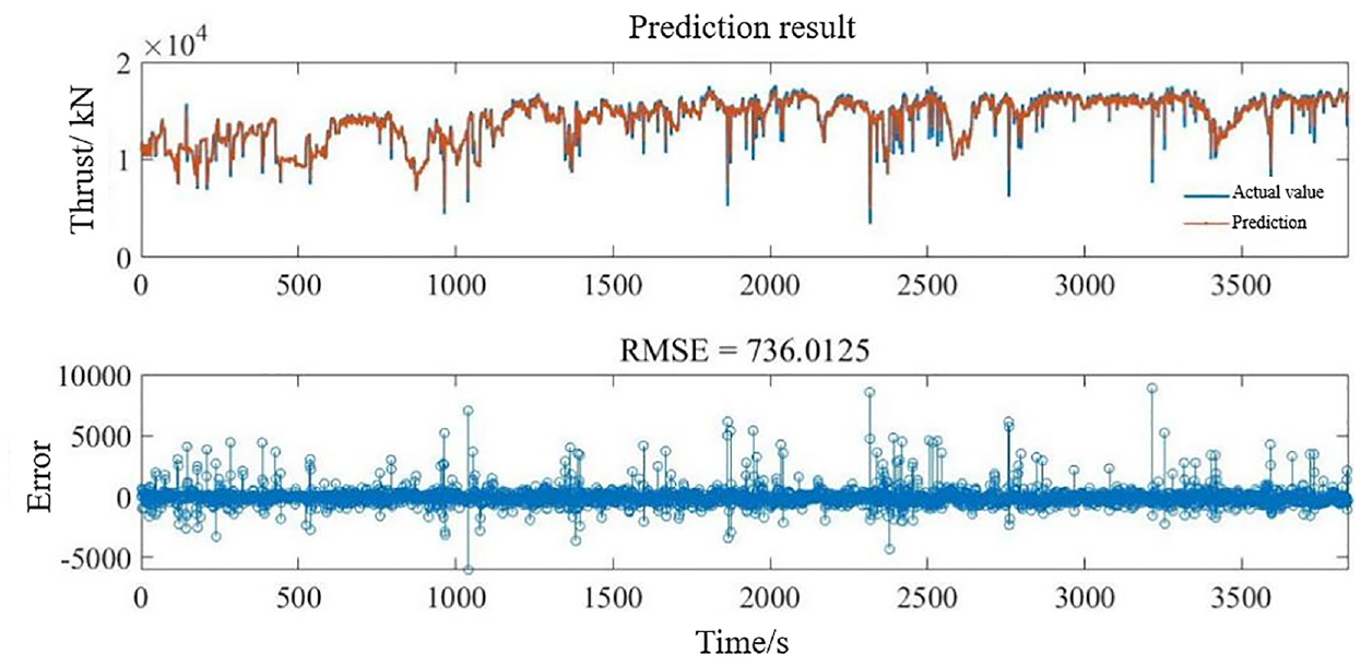
In order to study the overall prediction effect and stability of the model, 3840 sample size test set is used to test the model, and sample is input, where the sliding window width is 3. In indicates that ${x_{t - 2}^{(1)}, x_{t - 1}^{(1)}, x_{t}^{(1)}} (3 \leq t \leq 3839)$ is used to predict the $x_{t}^{(1)} (4 \leq t \leq 3840)$ data, then compare it with the actual value to obtain the prediction effect and accuracy, as shown in Figure 12.

Figure 12.

Prediction result of total thrust.

Figure 12 shows the comparison and error between the predicted data and the actual data of the total thrust test set, where the determination coefficient, MAPE, and RMSE is 0.8616, 3.1352%, and 736.0125. It can be seen from Figure 12 that the prediction error at the time of thrust value mutation point is relatively large. It may be caused by geological conditions, artificial operation, and other objective reasons. Moreover, the large total thrust value may result in parameters fluctuate greatly in a certain period of time to obtain inaccurate prediction. Overall, the predicted value is roughly the same as the actual value.

Establishment and verification of other parameter prediction models

The other four parameters are modeled and optimized by the above method. The influence of the input window width of each parameter prediction model on the prediction accuracy is shown in Figure 13, and influence of window width on prediction error is shown in Table 5. The optimal input window width and test accuracy of test set for each parameter are shown in the table, and the prediction effect is good.

Figure 13.

Test accuracy of each parameter prediction model with different window width: (a) cutter head torque, (b) gripper pressure, (c) cutter head speed, and (d) propulsion speed.

Table 5.

Test results of other parameters prediction model.

Window width	Cutter head torque	Gripper pressure	Cutter head speed	Propulsion speed
Evaluation index
Optimal input window width	3	10	10	3
RMSE	263.9842	1.0001	0.0646	5.5500
MAPE	7.9510	0.1122	0.3318	9.6900
R ²	0.9531	0.9982	0.9955	0.9678

Test of LSTM-SVM surrounding rock class prediction model

After the prediction model of five parameter characteristics is established, the prediction of surrounding rock class can be carried out. The data within the length of pile 2 + 500.0 to pile 2 + 710.0 were selected for testing because the surrounding rocks under this length includes class II, Class III, and Class IV. Among them, 2 + 500.0–2 + 610.0 + 635.0 is class II, 2 + 610.0–2 + 635.0 is class IV, and 2 + 635.0–2 + 710.0 is class III. It can verify the accuracy of the model as maximum as possible. According to the prediction process, firstly, extract the characteristics of the five kinds of boring parameters under the mileage, and then input them into the model according to their respective window widths for prediction. The prediction results are shown in Figure 14. Among them, the determination coefficient of the total thrust model is 0.9825, the cutterhead torque is 0.9396, the gripper pressure is 0.9974, the cutterhead rotate speed is 0.9843, and the advance speed is 0.9636. And the prediction effects are all good.

Figure 14.

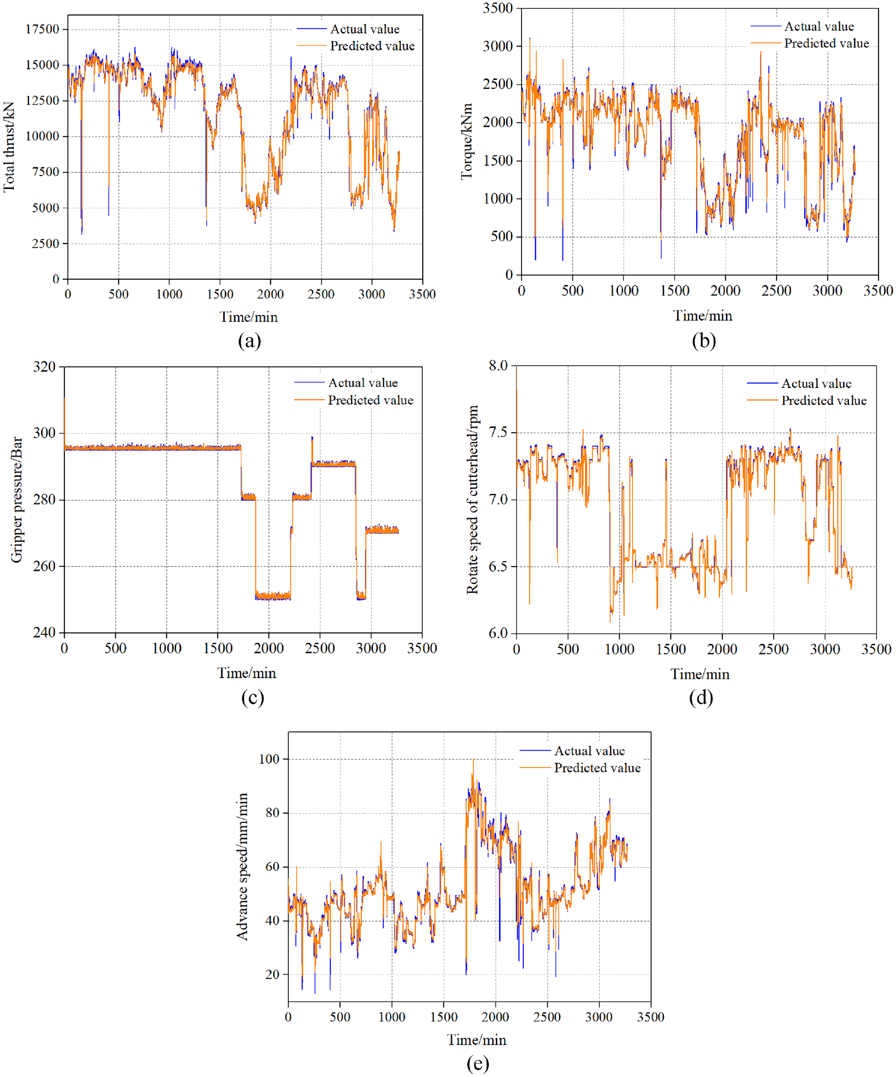
The prediction of five parameters: (a) total thrust, (b) cutter head torque, (c) gripper pressure, (d) cutter head speed, and (e) propulsion speed.

The surrounding rock is classified according to the prediction results of parameter feature values, and the results are shown in Figure 15(a). It can be seen that the overall prediction accuracy of the surrounding rock class prediction model can reach 86.0686%, which can provide reference for the prediction of the surrounding rock condition in the next stage. In order to further determine the source of the error, the actual value under this mileage is also substituted into the model for recognition. The result is shown in Figure 15(b), and the recognition accuracy is 87.0178%, which is similar to the prediction accuracy. Table 6 shows the identification prediction results of the surrounding rock classification using actual operating parameters. Therefore, the main error of the prediction model is the recognition error of the classification model, instead of the prediction effect of each parameter.

Figure 15.

The prediction results of the surrounding rock classification: (a) predicted operating parameters and (b) actual operating parameters.

Table 6.

The prediction results of the surrounding rock classification using actual operating parameters. (confusion matrix).

Predicted	Class II	Class III	Class IV	Class V	Total
Actual
Class II	1582	138	25	18	1763
Class III	9	1085	219	1	1314
Class IV	0	0	175	14	189

Conclusions

In this study, an intelligent prediction method for the surrounding rock classification model was proposed based on the TBM operating parameters. The prediction process consists of four steps: firstly, total thrust, cutterhead torque, gripper pressure, cutterhead rotate speed, and cutterhead advance speed are selected from the original data of TBM, through eliminating non-boring state and abnormal segment data and analyzing the correlation between each parameter and surrounding rock class. The feature vector of classification model is established, which is composed of the mean value of five operating parameters in each 60 s time window. Secondly, the LIBSVM is used for train and test of the classification model by means of 10-fold cross-verification method. The results show that the optimal penalty coefficient is 0.35, kernel parameter is 0.1768, the training accuracy of using this set of parameters is 98.25%, the accuracy of the test set is 92%. High accuracy of the test proves that the performance of LIBSVM algorithm is excellent. Thirdly, prediction model of five operating parameters is established based on LSTM network. The relationship among the prediction accuracy and time window width were studied, and the optimal input window width of each model has been verified by the test set. The results show that the decision coefficient of the total thrust model is 0.9825, the cutterhead torque is 0.9396, the gripper pressure is 0.9974, the cutterhead rotate speed is 0.9843, and the cutterhead advance speed is 0.9636. Finally, the LSTM-SVM model for the tunnel surrounding rock classification prediction is established, combining the parameter prediction model with the surrounding rock classification algorithm. The overall prediction accuracy of surrounding rock classification can reach 86.0686%. It can provide a prediction-based control method that operators can regulate the TBM operating parameters and formulate corresponding supporting measures beforehand rely on the surrounding rock classification prediction result. It can improve tunneling performance and safety of the TBM construction.

Footnotes

Handling Editor: Sharmili Pandian

Declaration of conflicting interests

The author(s) declared no potential conflicts of interest with respect to the research, authorship, and/or publication of this article.

Funding

The author(s) disclosed receipt of the following financial support for the research, authorship, and/or publication of this article: This work was supported by the Special funding support for the construction of innovative provinces in Hunan Province (2019GK1010).

ORCID iD

Mei Yang

References

Wei

Chu

, et al. Real-time rock mass condition prediction with TBM tunneling big data using a novel rock-machine mutual feedback perception method. J Rock Mech Geotech 2021; 13: 1311–1325.

Liu

Gong

Yang

, et al. A novel cutterhead off-stuck strategy for tunnel boring machine based on electro-hydraulic hybrid driving. Adv Mech Eng 2019; 11: 1–13.

Ling

Cheng

Tong

, et al. Research on rock breaking mechanism and load characteristics of TBM cutter based on discrete element method. Adv Mech Eng 2021; 13: 1–15.

Gong

Yin

, et al. TBM tunnelling under adverse geological conditions: an overview. Tunn Undergr Space Technol 2016; 57: 4–17.

Xue

Diao

, et al. A novel classification method of rock mass for TBM tunnel based on penetration performance. Chin J Rock Mech Eng 2018; S1: 3382–3391. (in Chinese)

Liu

Pan

, et al. A case study of TBM performance prediction using a Chinese rock mass classification system – Hydropower Classification (HC) method. Tunn Undergr Space Technol 2017; 65: 140–154.

Liu

Pan

, et al. Research advances of tunnel boring machine performance prediction models for hard rock. Chin J Rock Mech Eng 2016; 35: 2766–2786. (in Chinese)

Jamshidi

Prediction of TBM penetration rate from brittleness indexes using multiple regression analysis. Model Earth Syst Environ 2018; 4: 383–394.

Yagiz

Gokceoglu

Sezer

, et al. Application of two non-linear prediction tools to the estimation of tunnel boring machine performance. Eng Appl Artif Intell 2009; 22: 808–814.

10.

Qiu

Zhang

, et al. Prediction of surrounding rock classification in advance based on TSP203 system and GA-SVM. Chin J Rock Mech Eng 2010; 29(S1): 3221–3226. (in Chinese)

11.

Gao

Shi

Song

, et al. Recurrent neural networks for real-time prediction of TBM operating parameters. Autom Constr 2019; 98: 225–235.

12.

Wang

Gong

Yang

, et al. NSVR based predictive analysis of cutterhead torque for hard rock TBM. J Zhejiang Univ (Eng Sci) 2018; 52: 479–486. (in Chinese)

13.

Zheng

Chen

Zhang

Identification of loads on shield tunneling machines based on PSO-SVM method. Appl Mech Mater 2013; 392: 479–486.

14.

Tao

Qin

, et al. Rock mass type prediction for tunnel boring machine using a novel semi-supervised method. Measurement 2021; 179: 109545.

15.

Liu

Wang

, et al. Prediction of tunnel boring machine operating parameters using various machine learning algorithms. Tunn Undergr Space Technol 2021; 109: 103699.

16.

Zhang

LM.

Spatio-temporal feature fusion for real-time prediction of TBM operating parameters: a deep learning approach. Autom Constr 2021; 132: 103937.

17.

Wang

Zhu

, et al. An integrated parameter prediction framework for intelligent TBM excavation in hard rock. Tunn Undergr Space Technol 2021; 118: 104196.

18.

Huo

Jia

Liu

, et al. Advance prediction method for rock mass stability of tunnel boring based on deep neural network of time series. Proc IMechE, Part C: J Mechanical Engineering Science 2022; 236: 5618–5633.

19.

Feng

Chen

Hua

, et al. Tunnel boring machines (TBM) performance prediction: a case study using big data and deep learning. Tunn Undergr Space Technol 2021; 110: 103636.

20.

Kilic

Ikeda

Adachi

, et al. Soft ground tunnel lithology classification using clustering-guided light gradient boosting machine. J Rock Mech Geotech 2023; 15: 2857–2867.

21.

Heydari

Hamidi

Monjezi

, et al. An investigation of the relationship between muck geometry, TBM performance, and operational parameters: a case study in Golab II water transfer tunnel. Tunn Undergr Space Technol 2019; 88: 73–86.

22.

Koo

Cho

, et al. Using support vector machines to classify building elements for checking the semantic integrity of building information models. Autom Constr 2019; 98: 183–194.

23.

Hasan

Ahmad

Molla

MKI

. Protein subcellular localization prediction using multiple kernel learning based support vector machine. Mol Biosyst 2017; 13: 785–795.

Prediction method of TBM tunnel surrounding rock classification based on LSTM-SVM

Abstract

Keywords

Introduction

Methodology

Establishment of the database

Geological conditions project overview

Engineering data preprocessing

Correlation analysis between operating parameters and surrounding rock classes

Surrounding rock classification model based on LIBSVM

Classifier selection

Feature extraction and selection

Surrounding rock class prediction model based on LSTM-SVM

LSTM method

Data preprocessing and model evaluation indexes

Prediction model of operating parameters

Experiment results

Establishment of the database

Training based on LIBSVM model

Training of the prediction models for each feature parameter

Establishment and verification of the total thrust prediction model

Establishment and verification of other parameter prediction models

Test of LSTM-SVM surrounding rock class prediction model

Conclusions

Footnotes

Declaration of conflicting interests

Funding

ORCID iD

References