Sage Journals: Discover world-class research

Abstract

Since the spindle thermal error of CNC machine tools has a significant impact on machining precision, this paper introduces a unique approach for modeling spindle thermal error. Several key steps are involved in the proposed approach. First, the Fluke thermal imaging camera is employed for acquiring thermal image information of the spindle system. Second, the Gaussian filter is employed to denoise the thermal image sequence. Next, the temperature values at the measurement points are extracted from the thermal image sequence according to the mapping relationship between the grayscale value and the temperature value. Subsequently, critical temperature points are identified from thermal images using the density-based spatial clustering of applications with noise (DBSCAN) algorithm and the correlation coefficient method. Finally, the multi-verse optimized NARX neural network is employed to investigate the nonlinear prediction of thermal deformation. The research is conducted on the VMC-850E vertical machining center as the subject of study. The performance of the model is validated under conditions of idle spindle and 5000 r/min, comparing prediction results against traditional algorithms. The findings demonstrate that the non-contact measurement method based on thermal imaging successfully establishes the thermal error model, achieving a prediction accuracy of 0.1517 μm for the MVO-NARX model.

Keywords

CNC machine tool spindle system thermal error modeling thermal image multi-verse optimizer

Introduction

CNC machine tools, as the core equipment in the manufacturing industry, play a crucial role in determining a country’s manufacturing prowess and competitiveness. However, factors such as geometric, thermal, and tool wear-induced errors contribute to machining inaccuracies. Thermal errors emerge as the most significant source of deviation, accounting for roughly 40% to 70% of all machining error in machine tools.^1–3 The spindle is a critical component in machine tools responsible for generating substantial heat during operation. The thermal behavior of the spindle has a direct influence on the machining process and ultimately determines the precision of the final product. Therefore, mitigating thermal errors in CNC machine tool spindles is important to ensure exceptional precision and quality in the manufacturing process.

Extensive research suggests that neural network algorithms,^4,5 support vector machines,^6,7 and various other approaches can be utilized to formulate a precise thermal error prediction model, consequently diminishing thermal errors. A special technique was created by Liu et al.⁸ using BiLSTM deep learning to construct a model for predicting thermal errors. The maximum depth variation of the workpiece in the compensation experiment was reduced by over 85%. In the research conducted by Tian and Pan,⁹ they developed a prediction model utilizing self-organizing deep neural networks and integrated the Dropout mechanism into the model to improve its feature extraction capabilities. However, determining parameters for these models is typically based on empirical methods. Hence, different parameters can significantly impact the model’s accuracy. Therefore, some researchers have adopted intelligent optimization algorithms to optimize these methods’ parameters, improving the models’ predictive accuracy.

Huang et al.¹⁰ developed a thermal error correction model for a five-axis CNC machine tool, enhancing the neural network using the Shark Smell Optimization approach. The model was employed in a compensation experiment, leading to a notable 32% enhancement in workpiece machining accuracy. Li et al.¹¹ created a prediction model using least squares support vector machines (LS-SVM) and the aquila optimizer. The authors experimentally demonstrated that the proposed prediction model achieved an accuracy of over 94% for electric spindle thermal errors. Li et al.¹² developed the Particle Swarm Optimization Support Vector Machine (PSO-SVM) prediction model by optimizing the penalty factor and kernel function of the Support Vector Machine (SVM) using the particle swarm optimization (PSO) technique. Li et al.¹³ developed an electric spindle thermal error prediction model by optimizing the Elman neural network using the sparrow search algorithm (SSA). The improved model outperformed the unoptimized Elman neural network in terms of accuracy. Furthermore, it outperformed Elman neural network models based on particle swarm optimization.

Obtaining complete temperature field information for the machine tool spindle system is an important step in spindle thermal error modeling. Currently, the basic method for temperature field monitoring is mounting numerous temperature sensors on the spindle and building the thermal error model by combining temperature data from various measurement sites. Zhou et al.¹⁴ deployed 222 temperature sensors on a heavy-duty CNC gantry drilling machine to measure the temperature field information of the machine tool. The researchers employed the density peak clustering method to reduce the count of temperature measuring points to six, resulting in a reduction of data volume and enhancement of the thermal error prediction model’s robustness. Deng et al.¹⁵ devised and constructed a multi-source heterogeneous information acquisition experimental platform that integrates diverse sensor types. In this platform, the temperature field information of the machine tool was recorded using magnetic suction-type thermal resistance sensors, intelligent thermal characteristic testing, and a compensation device. However, such contact measurement methods require the arrangement of a large number of sensors during machine tool thermal characteristic experiments, leading to high costs. Furthermore, the placement of sensor measurement points is often determined using empirical methods, which may result in incomplete coverage of temperature-sensitive areas and consequently decrease the correctness of the model.

In light of these challenges, researchers have employed non-contact sensors to get temperature field data of the machine tool spindle system. Wu et al.¹⁶ utilized a combination of a thermal imaging camera and thermocouple sensors to capture the spindle’s temperature field. The prediction accuracy was between 90% and 93% using a deep convolutional neural network to foresee the heat deformation of the spindle in various orientations. Abdulshahed et al.¹⁷ developed a thermal error prediction model of a improved adaptive fuzzy neural reasoning system using a combination technique to identify important temperature points of various groups from thermal pictures.

In order to reduce the expense and complexity of performing thermal characteristic studies on machine tools and prevent overlooking important temperature measurement points, this study suggests a unique thermal error modeling technique based on thermal picture information extraction. Considering the influence of thermal hysteresis effects, it is acknowledged that thermal errors are not solely dependent on the current temperature state but are also impacted by historical temperature states. As a result, the NARX neural network model is introduced in this study. The NARX neural network incorporates a delay mechanism that attenuates the influence of thermal hysteresis effects compared to conventional intelligent prediction models. The basis for simulating thermal inaccuracy is provided by this neural network integration. On a VMC-850E vertical machining center, tests were done to demonstrate the viability of the suggested approach. Initially, a thermal imaging camera captured the spindle system’s temperature field image sequence, which was then subjected to appropriate preprocessing. Image information was accurately transformed into temperature information by establishing a mapping relationship between grayscale and temperature values in the thermal images. Subsequently, the DBSCAN algorithm and correlation coefficient approach were used to identify the locations of important temperature data points. The thermal error model was then updated to include these important temperature measurement sites as inputs. Finally, the MVO algorithm was leveraged to reasonably select parameters for the NARX neural network, leading to the construction of the MVO-NARX thermal error prediction model.

The remainder of this essay is divided into the following parts. In Section “Thermal error experiment and data preprocessing,” the thermal image sequence of machine tool spindle system is obtained by thermal error experiment, and the thermal image data is preprocessed. Section “Measurement point optimization and prediction model establishment” introduces the theoretical content of measuring point optimization and thermal error prediction model. In Section “Case study,” the model is verified. Final section presents the conclusions.

Thermal error experiment and data preprocessing

Construction of experimental platform

On the VMC-850E vertical machining center, the spindle’s thermal properties were investigated for this investigation. The experimental setup of the test platform is illustrated in Figure 1. The main hardware equipment for this experiment comprised the machining center body (Figure 1(d)), the intelligent thermal characteristics testing and compensation instrument for the CNC machine tool spindle system (Figure 1(a)), capacitance displacement device (Figure 1(b)), Fluke thermal imaging camera (Figure 1(c)), dedicated fixture for the five-point method, and a test bar (Figure 1(e)). The temperature field data of the spindle system were recorded by the Fluke TiS50 thermal imaging camera. According to Abdulshahed et al.¹⁷ and Lanc et al.,¹⁸ the emissivity of the thermal imaging camera was set to 0.95. Its value and other experimental parameters are set in Table 1. Displacement sensors were arranged according to Figure 1(e) to gather thermal displacement values in the z direction of the spindle system. In this experiment, the sampling time for the displacement sensor was set to 5 s. The specifications of the thermal imaging camera are shown in Table 2. Under idle conditions, the spindle system was maintained at a constant speed of 5000 r/min for approximately 5 h, during which temperature and displacement signal data were collected. The result of the displacement data acquisition is shown in Figure 2.

Figure 1.

Experimental platform: (a) intelligent thermal characteristics testing and compensation instrument, (b) capacitance displacement device, (c) fluke thermal imaging camera, (d) machining center body, and (e) displacement sensor position.

Table. 1.

Experimental parameter setting.

Parameter	Set value
Distance (m)	1.5
Emissivity	0.95
Ambient temperature (^oC)	30.8
Automatic capture time (min)	3

Table. 2.

Specifications of the thermal imaging camera.

Technical specification	Index
Operating temperature (^oC)	−10–+50
Relative humidity	10%–95%, non-condensing
Temperature range (^oC)	−20–450
Spectral range(μm)	7.5–14
Image resolution (pixel × pixel)	320 × 240

Figure 2.

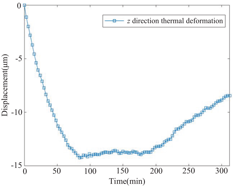
Spindle thermal displacement change.

Thermal image preprocessing

In this study, the machine tool spindle’s thermal picture sequence is obtained using a Fluke TiS50 thermal imaging camera, from the cooling condition to the thermal equilibrium state. In order to correctly collect the temperature information at any place of the spindle system and to enable the quantitative measurement and analysis of the temperature value, this study performed denoising and temperature information extraction pre-processing on the generated thermal image sequence.

Thermal image denoising

The ambient temperature, humidity, and air emissivity can all have an impact on the thermal picture that the thermal imaging camera captures, which increases the amount of noise in the image. This noise can potentially introduce inaccuracies in the temperature values of discrete points. Hence, this study employs a Gaussian filter, which preserves the overall gray distribution characteristics of the thermal image while removing noise by denoising the image sequence.

Gaussian filtering^19,20 employs a filter kernel function to carry out convolution operation with the image to be processed, in which the filter kernel function is mainly set according to the filter parameters. The calculation formula of the Gaussian filter kernel function is as follows:

G (p, q) = \frac{1}{2 π σ^{2}} e^{- \frac{{(p - p_{0})}^{2} + {(q - q_{0})}^{2}}{2 σ^{2}}}

(1)

where $G (p, q)$ is the grayscale value of the denoised image at the pixel position $(p, q)$ , $p_{0}$ , $q_{0}$ is the local filtering central point, and $σ$ represents the smoothing scale parameter.

Thermal image temperature extraction

Pixel is the most basic unit of an image, and each gray image is composed of pixels with different gray values. The essence of an infrared image is a gray image, and data information of its pixels is converted from infrared thermal radiation energy. Therefore, there is a certain mapping relationship between the gray value of each pixel in the image and the temperature value. Suppose that the mapping function between the grayscale value and temperature value²¹ is

T = \sum_{k = 0}^{n} a_{k} G^{k}

(2)

where T represents the measured temperature value of the pixel, G represents the grayscale value of the pixel of the thermal image, k is the fitting degree, $a_{k}$ and is the least square coefficient.***

The coefficient $a_{k}$ must be obtained to acquire the specific expression of equation (2). The least squares coefficient and RMSE error value for this study may be calculated using the least squares principle and the RMSE error formula,²² as shown in Table 3. The root-mean-square error changes with the level of fit, as seen in Table 3. RMSE is the smallest when k = 2; hence, quadratic fitting is adopted, and the obtained fitting coefficient is $a_{0} = 32.40, a_{1} = 0.06203, a_{2} = - 5.817 \times 10^{- 5}$ . Equation (2) can be rewritten as equation (3).

T = - 5.817 \times 10^{- 5} \times G^{2} + 0.06203 \times G + 32.40

(3)

Table. 3.

$a_{k}$ and its corresponding root-mean-square error.

K	RMSE	a ₀	a ₁	a ₂	a ₃
1	0.3046	32.85	0.04883	–	–
2	0.1342	32.40	0.06203	−5.817 × 10⁻⁵	–
3	0.1348	32.43	0.05967	−3.090 × 10⁻⁵	−8.004 × 10⁻⁸

To check the precision of the fitting formula, an additional 20 groups of data were randomly chosen as test samples within the grayscale value of the thermal image sequence’s fluctuation range. The temperature associated with each gray value was then approximated using the resulting fitting equation (3), and the residual difference between the estimated value and the observed value was determined to assess the fitting impact. The particular evaluation outcomes are displayed in Table 4. According to Table 4, the absolute maximum of residual is 0.24^oC, the absolute minimum is 0.01^oC, the absolute average is 0.1^oC, the maximum relative error is 0.7%, the minimum is 0.02%, the absolute value of residual is less than 0.3^oC, and the relative error is less than 5%. It can be concluded that the temperature value fitting based on the least square method exhibits good accuracy.

Table. 4.

Test sample estimation.

Sample number	Gray value	Measured value (^oC)	Estimated value (^oC)	Residual value (^oC)
1#	6	32.84	32.77	0.07
2#	18	33.63	33.50	0.13
3#	26	34.03	33.97	0.06
4#	32	34.43	34.33	0.10
5#	45	34.83	35.07	0.24
6#	52	35.23	35.47	0.24
7#	66	36.04	36.24	0.20
8#	79	36.82	36.94	0.12
9#	92	37.63	37.61	0.02
10#	99	38.02	37.97	0.05
11#	109	38.42	38.47	0.05
12#	124	39.22	39.20	0.02
13#	137	40.02	39.81	0.21
14#	151	40.42	40.44	0.02
15#	160	40.82	40.84	0.02
16#	180	41.64	41.68	0.04
17#	190	42.04	42.09	0.05
18#	204	42.44	42.63	0.19
19#	220	43.24	43.23	0.01
20#	240	44.12	43.94	0.18

Measurement point optimization and prediction model establishment

Measurement point optimization

For the modeling of thermal inaccuracy, locating temperature-sensitive locations is of utmost importance. If there are too many measuring points, multicollinearity problems may arise among temperature variables, and if there are too few, the relationship between temperature and thermal inaccuracy may not be fully established. The prediction power of thermal error models can also be hampered by an irrational arrangement of measurement locations. In order to filter important temperature measurement locations, this study uses the DBSCAN clustering technique and correlation coefficient approach, following the concept of measurement point optimization as outlined in Zhou et al.¹⁴

DBSCAN algorithm

One example of a density-based clustering method is the DBSCAN algorithm, which has two parameters: a minimal number of points (Minpts) and a neighborhood radius (Eps). Without specifying the number of clusters, the method may cluster data sets of any form and identify outliers.²³ To make temperature measurement points more accurate, utilize the DBSCAN method. The following detailed stages make up the algorithm:

(1) Input temperature point temperature vector $D = {T_{1}, \dots, T_{n}}$ , where n denotes how many measurement points were generally retrieved from the thermal picture.

(2) The Eps neighborhood subsample set of all temperature samples $T_{i}$ is measured via distance. If the number of sample sets meets $N_{Eps} (T_{i}) \geq Minpts$ , the measuring point $T_{i}$ is added to the collection of core object samples $Ω$ ; if not, the measuring point $T_{i}$ is marked as a boundary or noise point.

(3) A test point core object $T_{i}$ is randomly selected in the core object set $Ω$ . A new sample set $C_{1}$ is established, and all the test points in its Eps neighborhood are added to the sample set $C_{1}$ . The measuring points in the Eps neighborhood are checked for all measuring points in $C_{1}$ and added to $C_{1}$ . The check is repeated until no new test points can be added. The object collection is updated as $Ω = Ω - C_{1}$ .

(4) A test point core object $T_{i}$ is randomly selected in the updated core object set $Ω$ , and step (3) is repeated until the core object $Ω$ is empty. The sample set partitioning result ${C_{1}, C_{2}, \dots, C_{n}}$ is the output.

Correlation coefficient method

The numerical value of the Pearson correlation coefficient, which ranges from [0,1], is used to assess the relationship between each temperature measurement point and thermal deformation. The closer the absolute value was to 1, the stronger the correlation was Wei et al.²⁴ The correlation coefficient $ρ_{x_{k}, y}$ between the kth temperature measurement point and thermal deformation can be represented as follows:

ρ_{x_{k}, y} = \frac{\sum_{m = 1}^{n} [x_{k, m} - {\bar{x}}_{k}] [y_{m} - \bar{y}]}{\sqrt{\sum_{m = 1}^{n} {[x_{k, m} - {\bar{x}}_{k}]}^{2} {[y_{m} - \bar{y}]}^{2}}}

(4)

where $x_{k}$ denotes the temperature of the kth temperature measuring point; y represents the thermal deformation value; ${\bar{x}}_{k}$ and $\bar{y}$ represent the mean value of the kth measurement point and thermal deformation, respectively; $x_{k, m}$ and $y_{m}$ are the kth temperature measurement point and the mth measurement value of thermal deformation respectively.

Optimized result

As shown in Figure 3, a total of 152 locations in the thermal picture were determined to be main temperature measurement sites. The temperature values of the chosen measurement locations are then calculated using the fitting equation (3). Additionally, Figure 4 extracts and displays the temperature trends of certain temperature monitoring locations.

Figure 3.

152 measuring point positions obtained from thermal images.

Figure 4.

The temperature value of some measuring points and its changing trend.

The multicollinearity among these points may arise due to the substantial number of obtained measurement points, potentially reducing the model’s prediction accuracy. Therefore, the measurement points must be optimized. The main steps are as follows:

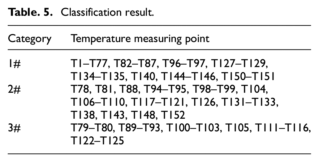
(1) the 152 acquired measurement points were segregated into three categories using the DBSCAN algorithm, with the specific classification results detailed in Table 5.

(2) To calculate the association between the temperature measurement points and the thermal deformation data within each category, the correlation coefficient technique was used, and the correlations were ordered appropriately.

(3) The key temperature points were determined for each category founded on the sorting outcomes of different temperature measurement points and the clustering findings of various points. Specifically, T140 emerged as the significant temperature point for the first category. T152 was identified as the key point for the second category, and T116 for the third category. The optimized positions of these measurement points are illustrated in Figure 5.

Table. 5.

Classification result.

Category	Temperature measuring point
1#	T1–T77, T82–T87, T96–T97, T127–T129, T134–T135, T140, T144–T146, T150–T151
2#	T78, T81, T88, T94–T95, T98–T99, T104, T106–T110, T117–T121, T126, T131–T133, T138, T143, T148, T152
3#	T79–T80, T89–T93, T100–T103, T105, T111–T116, T122–T125

Figure 5.

The optimized location of the measuring point.

Establishment of MVO-NARX prediction model

The thermal error modeling approach in this inquiry entails obtaining temperature values from critical temperature measurement locations in thermal pictures. With its memory for past data, the NARX neural network is well-suited for modeling. The NARX neural network was fed with the optimal temperature values of the selected important data locations. Simultaneously, the output variable was the thermal deformation in the z-direction of the main axis system. Concurrently, the MVO method is used to optimize the network’s parameters, culminating in the development of the MVO-NARX thermal error prediction model.

NARX neural network

The NARX neural network, which consists of input, hidden, and output layers, is a form of dynamic neural network built for periods of time prediction. The delay and feedback mechanisms are incorporated in the NARX neural network. Thus, its memory capability for historical data is enhanced by preserving and incorporating the previous moment’s data into the next time step’s calculations.^25,26 The mathematical expression is as follows:

\begin{matrix} y (p) = f (y (p - 1), y (p - 2), \dots y (p - D_{o}), \\ x (p - 1), x (p - 2), \dots x (p - D_{i})) \end{matrix}

(5)

where y(p − 1) indicates the output variable at time p − 1, x(p − 1) represents the input variable at time p − 1, $D_{o}$ is the output delay, and $D_{i}$ appears the input delay.

The NARX neural network operates in two modes. The first is the Series-Parallel mode (Open-loop), in which the intended output is known and is given back to the input directly. Using known input and output data, the network learns its functional connection. The second option is Parallel (Closed-loop), in which the intended output is unknown. This mode extends the Series-Parallel mode by adding a feedback loop in which the output signal is transmitted back into the network as an input, altering the prediction of the output signal. This paper adopts the Series-Parallel mode for network training and the Parallel mode for testing and prediction since the open-loop network can efficiently learn the functional relationship between input and output, and the closed-loop network is better at capturing the dynamic correlation and historical information between signals in the prediction process.

MVO algorithm

MVO is a swarm intelligence optimization algorithm founded on the multi-verse theory. It was jointly offered by S. Mirjalili, SM. Mirjalili, and A. Hatamlou in 2015. The multi-verse theory introduces three core notions: white holes, black holes, and wormholes.²⁷ In the multi-verse space, white holes possess strong repulsive forces capable of releasing all objects. On the contrary, black holes possess incredibly strong gravitational forces capable of absorbing all matter. Meanwhile, wormholes function as pathways that link disparate universes, enabling the transfer of objects between them. The combined interaction of these three concepts causes the entire multi-verse population to reach a stable state.

Like other intelligence optimization algorithms, the MVO algorithm follows a two-stage optimization process, involving exploration and exploitation. During the exploration stage, the white and black holes are active, while the exploitation stage involves the utilization of wormholes.

In order to build the MVO algorithm, a mathematical model is created that takes into account the motion behavior of the multiverse population. Each universe in this mathematical model is seen as a potential solution to an optimization issue, and the pace at which each universe expands is inversely related to the desired result of the optimization problem. The solution is updated in an iterative procedure until the global optimization objective is attained. According to the literature,²⁶ the MVO algorithm’s operational phases are as follows:

(1) A group of n universes is initialized to conduct the search in the d-dimensional target space, as represented in equation (6).

\begin{matrix} U = [\begin{matrix} U_{1} \\ U_{2} \\ ⋮ \\ U_{n} \end{matrix}] = [\begin{matrix} a_{1}^{1} & a_{1}^{2} & \dots & a_{1}^{d} \\ a_{2}^{1} & a_{2}^{2} & \dots & a_{2}^{d} \\ ⋮ & ⋮ & ⋮ & ⋮ \\ a_{n}^{1} & a_{n}^{2} & \dots & a_{n}^{d} \end{matrix}] \end{matrix}

(6)

where n is the population size (number of universes/candidate solutions), d represents the number of objects (variables), $U_{i} = (a_{i}^{1}, a_{i}^{2}, \dots, a_{i}^{d})$ represents the ith universe, and $a_{i}^{j}$ represents the jth object of the ith universe.

(2) The objects of the universes are exchanged to establish a white/black hole tunnel. During each iteration, the universes are sorted based on their expansion rate (fitness), and a white hole is selected using a roulette wheel mechanism following the procedure outlined in equation (7).

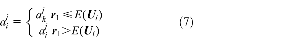
a_{i}^{j} = {\begin{matrix} a_{k}^{j} r_{1} \leq E (U_{i}) \\ a_{i}^{j} r_{1} > E (U_{i}) \end{matrix}

(7)

where $E (U_{i})$ represents the normalized expansion rate of the ith universe, $r_{1}$ is a random number within the range of [0,1], and $a_{k}^{j}$ represents the jth object of the kth universe selected by the roulette wheel mechanism.

(3) This algorithm introduces the wormhole existence probability (WEP) and travel distance ratio (TDR) to perform more precise local searches within the obtained global best range. The WEP linearly increases during iteration while the TDR continuously decreases. The update principles for these two parameters follow equations (8) and (9).

WEP = WE P_{min} + l \times (\frac{WE P_{max} - WE P_{min}}{L})

(8)

T D R = - \frac{l^{1 / p}}{L^{1 / p}}

(9)

where l is the current count of iterations, L denotes the maximum count of iterations, and p is the accuracy of iterative development, and the value is 6.

(4) The positions of the universes are updated, and the optimal individual is searched for. The universes, irrespective of the expansion rate’s magnitude, actively drive internal objects to converge toward the current optimal universe.

\begin{matrix} a_{i}^{j} = {\begin{matrix} {\begin{matrix} A_{j} + TDR \times ((b_{uj} - b_{lj}) \times r_{4} + b_{lj}) r_{3} < 0.5 \\ A_{j} - TDR \times ((b_{uj} - b_{lj}) \times r_{4} + b_{lj}) r_{3} \geq 0.5 \end{matrix} & r_{2} < WEP \\ a_{i}^{j} & r_{2} \geq WEP \end{matrix} \end{matrix}

(10)

where $A_{j}$ represents the jth object of the current optimal universe, $b_{lj}$ and $b_{uj}$ refer to the lower limit and upper limit of $a_{i}^{j}$ , respectively, and $r_{2}$ , $r_{3}$ , $r_{4}$ are random numbers between [0,1].

The internal logical structure of MVO is illustrated in Figure 6.

Figure 6.

Flowchart of the structure of the MVO.

Establishment of MVO-NARX model

The NARX neural network’s input delay order $D_{i}$ , output delay order $D_{o}$ , and the count of neurons h inside the hidden layer are all essential characteristics.

These parameters are typically determined using empirical methods or repeated experiments. Setting these values as too low may result in the network failing to capture important temporal relationships in the data. On the other hand, setting them too high may increase the training process and lead to overfitting. The MVO algorithm requires adjusting only a few parameters and exhibits strong adaptability. The algorithm can self-adjust based on feedback during the search process, aiming to find better solutions throughout the iterations. Additionally, the MVO algorithm can conduct simultaneous searches in multiple virtual universes, increasing the possibility of finding the global optimal solution. The MVO algorithm has demonstrated successful applications in various classical engineering design issues. The MVO approach is used in this work to enhance the predictive accuracy of neural networks and to explore their structural parameters in quest of the optimal parameter setting. The following are the operational stages for enhancing the NARX neural network using the MVO algorithm:

(1) Create the universe’s population. Determine the count of universes n, the upper and lower limits of the input and output delay orders, as well as the count of hidden layer neurons h, the search space dimension d, and M, the number of iterations at the most.

(2) The mean squared error (MSE), which acts as the optimization algorithm’s goal, is the fitness function. Each solution’s performance is evaluated by training and testing the NARX neural network and calculating its mean squared error.

(3) Update the universe state. Compute the fitness values for each universe and arrange them in ascending order. The white hole universe is chosen using a roulette wheel selection technique. White holes, black holes, and wormholes all operate by updating the location of the universe.

(4) The loop is terminated. Steps (2) and (3) are repeated until the maximum iteration count is reached. The best position of the universe is the output, which represents the optimal parameter combination ${D_{i}, D_{o}, h}$ .

(5) The optimal parameter combination is applied to the NARX neural network for thermal error prediction.

Case study

The obtained temperature values at measurement points and thermal deformation values from the experiment were aligned on the time axis, resulting in 105 sampling samples. Each sample corresponds to the machine tool’s condition at a particular time point. The temperature values at the measurement places are used as inputs and the recorded thermal deformation values are used as outputs to develop a NARX thermal error prediction scheme. The MVO approach was adopted to look for model parameters and improve the model’s predictive capability. The predicted outcomes were contrasted with those produced by traditional algorithms. To evaluate the model’s stability and efficacy, the 105 samples were separated into a training set and a testing set in a 7:3 ratio. The testing set was utilized in this study to evaluate the model’s predictability and stability whereas the training set was adopted to create the model and do early assessments of its efficacy. The four phases that make up the full thermal error modeling approach built around thermal imaging process are described in this study. Figure 7 reveals the comprehensive process of the approach.

(1) A thermal imaging camera and displacement sensor were used to gather information from the machining center’s spindle system.

(2) The mapping relationship between grayscale value and temperature value of thermal image was obtained by using least square principle. The thermal picture was then denoised using a Gaussian filter to reduce any potential influence from temperature data extraction.

(3) After the temperature values of the locations for measuring on the infrared picture were recorded in accordance with the relationship, the temperature measurement sites were screened using the correlation coefficient methodology and the DBSCAN method.

(4) By modifying the NARX neural network’s parameters using the optimized measurement point as input and z-direction thermal deformation as output, the thermal error prediction model for MVO-NARX is created.

Figure 7.

Flowchart of the proposed method.

Establishment of model

The training set for the model was the first 75 data from the thermal error experiment. To enhance the neural network’s parameters, we used the MVO method. For this optimization process, we set the search ranges for the input and output delay orders as [1,5], and the search range for the number of hidden layer neurons as [1,10]. Furthermore, we set the maximum iteration count to 300 and the population size to 30. The final determined parameter combination was obtained via multiple experimental simulations as {4,1,8}, the corresponding fitness curves were displayed in Figure 8(c). The fitness curves of the Genetic Algorithm (GA) and Particle Swarm Optimization (PSO) Algorithm were illustrated in Figure 8(a) and (b), respectively. It was evident from the figures that all three parameter optimization algorithms achieved convergence within 150 generations. Their respective fitness values were 0.0735, 0.0388, and 0.0299. Notably, the MVO algorithm showed the lowest fitness value, reducing it by 59.32% and 22.94% compared to GA and PSO algorithms, respectively. This demonstrated that the MVO approach recommended in this article might provide better results throughout the optimization phase and was useful in the growth of a thermal error model.

Figure 8.

Fitness curves for different optimization algorithms: (a) fitness curve of GA method, (b) fitness curve of PSO method, and (c) fitness curve of MVO method.

Validation of model

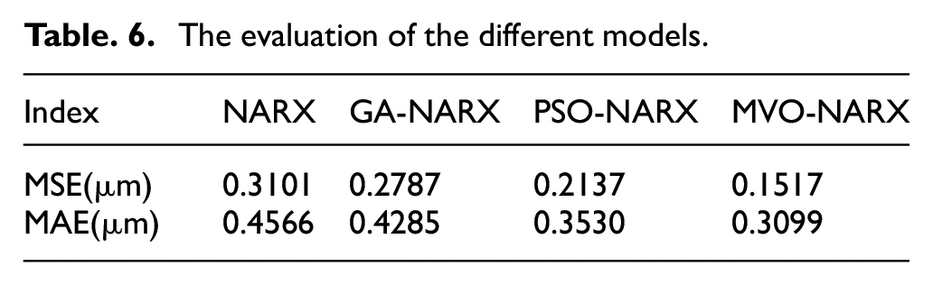
To confirm the efficacy of the predictive model developed during the training procedure, the model was assessed using the testing set. The testing set consisted of the latest 30 samples from the experimental data. The developed model was run using the optimal temperature values acquired from the measurement locations, and a comparison between the anticipated and observed thermal deformation values was done. A comparative study was conducted involving the unoptimized NARX model, the NARX neural network improved through genetic algorithm and particle swarm optimization, and the proposed model. This was done to assess the suggested MVO-NARX thermal error model’s predictive capability and generalizability. Figure 9 displays the forecasts produced by the four distinct models. Utilizing mean square error (MSE) and mean absolute error (MAE), the model’s prediction ability is evaluated. Superior prediction accuracy is shown by lower MSE and MAE values. Table 6 displays the evaluation’s findings. Figure 10 shows the predicted residual curves for each model. The thermal error model’s predictive ability is considered better when the residual curve approaches the zero axis closely.

Figure 9.

Predictions from different models: (a) prediction results of NARX model, (b) prediction results of GA-NARX model, (c) prediction results of PSO-NARX model, and (d) prediction results of MVO-NARX model.

Table. 6.

The evaluation of the different models.

Index	NARX	GA-NARX	PSO-NARX	MVO-NARX
MSE(μm)	0.3101	0.2787	0.2137	0.1517
MAE(μm)	0.4566	0.4285	0.3530	0.3099

Figure 10.

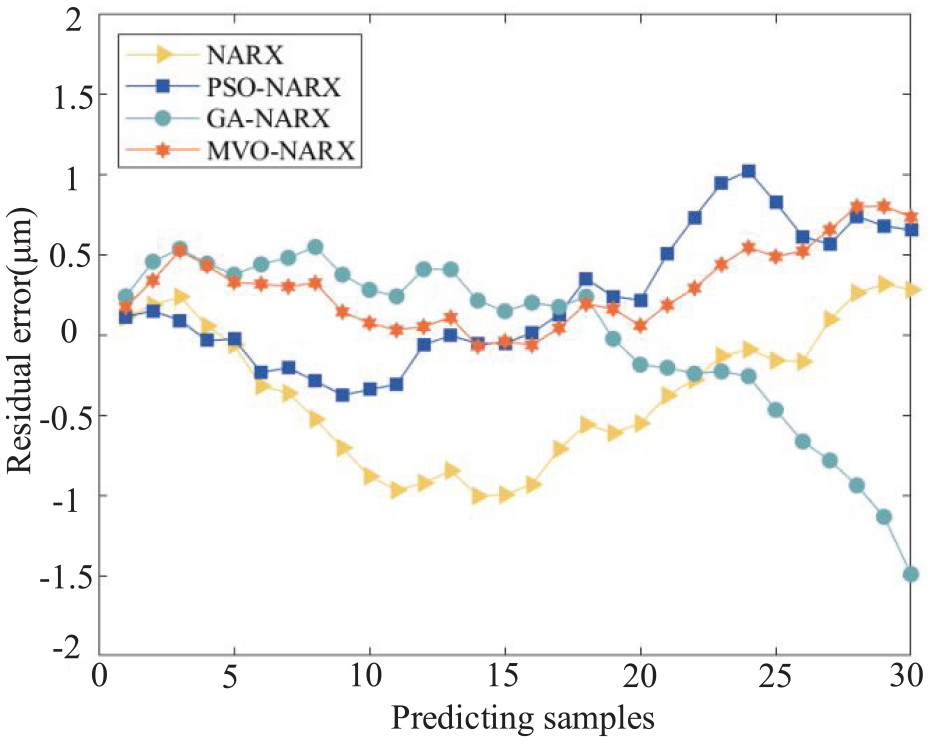
Prediction residual curves of different models.

The prediction results produced by the NARX neural network model closely match the observed values, as shown in Figures 9 and 10, and Table 6. The NARX neural network thermal error model suggests a certain amount of predictive potential when both the mean square error (MSE) and mean absolute error (MAE), which are both below 0.5 μm, are included. Additionally, by applying the multi-dimensional universe optimization technique to adjust the structural variables of the neural network, a more precise prediction model was produced. The MVO-NARX model’s residual curve shows a tighter alignment with the zero axis than the other models, and MSE and MAE are lower than the comparable values of the NARX, GA-MVO, and PSO-NARX models.

In summary, it can be said that the thermal error model developed through clever optimization algorithms effectively and efficiently captures the correlation between temperature and thermal inaccuracy based on a comparative assessment of the prediction outcomes from the NARX model and the actual thermal deformation measurements. Furthermore, when compared to models created using the GA and PSO algorithms, the MVO algorithm-based model exhibits greater prediction accuracy.

Conclusions

A thermal image-based MVO-NARX thermal error model is developed in this work to limit thermal errors in CNC machine tools and overcome the difficulty of incomplete temperature measurement point selection caused by contact measurements. To show the availability of thermal pictures and assess the prediction impact of a single prediction model and a mixed prediction model, machine tool thermal error tests were performed using the VMC-850E machining center. The following important results are possible:

(1) The mapping relationship between the gray level of thermal image and the temperature value was successfully determined by the principle of least squares, and the relative error between the measured value and the estimated value was less than 5%. The conversion of image information to temperature information was realized, which was convenient for the quantitative measurement and analysis of temperature data. The obtained temperature data were seamlessly integrated into the subsequent thermal error model, enabling accurate thermal error predictions for the CNC machine tool spindle system.

(2) The combination optimization method using DBSCAN algorithm and correlation coefficient method successfully reduced the count of measurement points from 152 to three, eliminated multicollinearity between variables, and decreased the dimension of the model.

(3) As inputs, the NARX thermal error prediction model receives optimal temperature values at measurement sites, as well as associated thermal error values. The structural parameters of the NARX neural network were improved using MVO. The investigation shows that the MVO-NARX model outperforms the NARX, GA-NARX, and PSO-NARX models in terms of parameter setting and prediction accuracy, with average square error cuts of roughly 51%, 46%, and 29%, respectively. Therefore, MVO-NARX prediction model was more proper for thermal error prediction of CNC machine tool spindle system.

Footnotes

Handling Editor: Dr Himani Dewan

Author contributions

Conceptualization, Xiaolei Deng; methodology, Wanjun Zhang, Yong Chen, and Jianchen Wang; validation, Yue Han; formal analysis, Yue Han; investigation, Yushen Chen and Chengzhi Fang; resources, Xiaolei Deng; writing—original draft preparation, Yue Han; writing—review and editing, Yushen Chen; supervision, Xiaolei Deng.

Declaration of conflicting interests

The author(s) declared no potential conflicts of interest with respect to the research, authorship, and/or publication of this article.

Funding

The author(s) disclosed receipt of the following financial support for the research, authorship, and/or publication of this article: This research was financially supported by the National Natural Science Foundation of China (52175472 & 62302263), Zhejiang Provincial Natural Science Foundation of China (LD24E050011 & LGG22E050031 & LZY21E050002 & ZCLTGS24E0601), Natural Science Foundation of Zhejiang Province for Distinguished Young Scholars (LR22E050002), and Science and Technology Plan Project of Quzhou (2022K90 & 2021K41 & ZD2022188).

ORCID iD

Yue Han

References

Bai

, et al. A review of thermal error modeling methods for machine tools. Appl Sci 2021; 11: 5216.

Deng

Lin

Wang

, et al. Review on thermal design of machine tool spindles. Opt Precis Eng 2018; 26: 1415–1429.

Liu

Wang

, et al. Review on thermal error compensation for feed axes of CNC machine tools. J Mech Eng 2021; 57: 156–173.

Zhao

Mei

, et al. Thermal error compensation based on genetic algorithm and artificial neural network of the shaft in the high-speed spindle system. Proc Inst Mech Eng Part B J Eng Manuf 2017; 231: 753–767.

Zhu

Xiang

Yang

. Novel thermal error modeling method for machining centers. Proc Inst Mech Eng Part C J Mech Eng Sci 2015; 229: 1500–1508.

Dai

Wang

Xiong

, et al., Thermal error modelling of motorised spindle in large-sized gear grinding machine. Proc Inst Mech Eng Part B J Eng Manuf 2017; 231: 768–778.

Miao

Gong

Niu

, et al. Robustness of thermal error compensation modeling models of CNC machine tools. Int J Adv Manuf Technol 2013; 69: 2593–2603.

Liu

, et al. Thermal error modeling based on BiLSTM deep learning for CNC machine tool. Adv Manuf 2021; 9: 235–249.

Tian

Pan

. An unsupervised regularization and dropout based deep neural network and its application for thermal error prediction. Appl Sci 2020; 10: 2870.

10.

Huang

Liu

Liao

, et al. Thermal error modeling of numerical control machine tools based on neural network by optimized SSO algorithm. J Northeast Univ 2021; 42: 1569–1578.

11.

Wang

Zhu

, et al. Thermal error modeling of high-speed electric spindle based on aquila optimizer optimized least squares support vector machine. Case Stud Therm Eng 2022; 39: 102432.

12.

Zhu

, et al. Thermal error modeling of electric spindle based on particle swarm optimization-SVM neural network. Int J Adv Manuf Technol 2022; 121: 7215–7227.

13.

Zhu

Dai

, et al, Thermal error modeling of motorized spindle based on Elman neural network optimized by sparrow search algorithm. Int J Adv Manuf Technol 2022; 121: 349–366.

14.

Zhou

Liu

, et al. The selection of key temperature measurement points for thermal error modeling of heavy-duty computer numerical control machine tools with density peaks clustering. Adv Mech Eng 2019; 11: 1–11.

15.

Deng

Chen

Guo

, et al. Multi-source heterogeneous information acquiring test experiment and platform construction for CNC machine tool. Opt Precis Eng 2022; 30: 1440–1451.

16.

Xiang

. Spindle thermal error prediction approach based on thermal infrared images: a deep learning method. J Manuf Syst 2021; 59: 67–80.

17.

Abdulshahed

Longstaff

Fletcher

, et al. Thermal error modelling of machine tools based on ANFIS with fuzzy c-means clustering using a thermal imaging camera. Appl Math Modell 2015; 39: 1837–1852.

18.

Lanc

Zeljković

Živković

, et al. Determination of emissivity of brass alloy using infrared thermographic technique. Mater Geoenviron 2018; 65: 115–121.

19.

Ito

Xiong

. Gaussian filters for nonlinear filtering problems. IEEE Trans Autom Control 2000; 45: 910–927.

20.

, et al. A numerical-integration perspective on gaussian filters. IEEE Trans Signal Process 2006; 54: 2910–2921.

21.

Zhang

Chen

, et al. A method for reducing the influence of measuring distance on infrared thermal imager temperature measurement accuracy. Appl Therm Eng 2016; 100: 1095–1101.

22.

Fang

Chen

Deng

, et al. Denoising method of machine tool vibration signal based on variational mode decomposition and Whale-Tabu optimization algorithm. Sci Rep 2023; 13: 2100.

23.

Bryant

Cios

. RNN-DBSCAN: a density-based clustering algorithm using reverse nearest neighbor density estimates. IEEE Trans Knowl Data Eng 2018; 30: 1109–1121.

24.

Wei

Qian

Feng

, et al. Robust modeling method for thermal error of CNC machine tools based on partial least squares algorithm. Chin J Sci Instrum 2021; 42: 34–41.

25.

Louzazni

Mosalam

Cotfas

. Forecasting of photovoltaic power by means of non-linear auto-regressive exogenous artificial neural network and time series analysis. Electronics 2021; 10: 1953.

26.

Wei

Wang

, et al. An indirect remaining useful life prediction of lithium-ion batteries based on a NARX dynamic neural network. Chin J Eng 2022; 44: 380–388.

27.

Mirjalili

Hatamlou

. Multi-verse optimizer: a nature-inspired algorithm for global optimization. Neural Comput Appl 2016; 27: 495–513.

Multi-verse optimizer for thermal error modeling approach of spindle system based on thermal image

Abstract

Keywords

Introduction

Thermal error experiment and data preprocessing

Construction of experimental platform

Thermal image preprocessing

Thermal image denoising

Thermal image temperature extraction

Measurement point optimization and prediction model establishment

Measurement point optimization

DBSCAN algorithm

Correlation coefficient method

Optimized result

Establishment of MVO-NARX prediction model

NARX neural network

MVO algorithm

Establishment of MVO-NARX model

Case study

Establishment of model

Validation of model

Conclusions

Footnotes

Author contributions

Declaration of conflicting interests

Funding

ORCID iD

References