
Abstract
The dynamic coefficients (dynamic stiffness coefficient and dynamic damping coefficient) of gas foil bearings (GFBs) are important for transient dynamics calculation and stability analysis of the GFBs-rotor system. Although the perturbation method can be used to calculate the dynamic coefficients, it can only consider a single whirl ratio. Moreover, the whirl ratio is assumed and not practical. Therefore, this paper proposes an identification method of dynamic coefficients of GFBs by simulated excitation. Firstly, based on single journal-single GFB model considering gas-structure interaction by coupled fields, harmonic excitations were applied to the rotor to obtain the shaft orbit. Next, frequency response function method and equivalence coefficient method were used to identify dynamic coefficients. The former method is suitable for the case where response and excitation are same frequency, namely linear problem. The latter method is fit for the situation in which the response has multiple frequency components, namely nonlinear problem. Finally, examples were carried out, and the results from different methods were compared and analyzed. This research work lays a theoretical foundation for the design of the GFBs-rotor system.
Introduction
GFBs are widely used in high efficiency blowers, aircraft air circulation cooling systems, micro fuel cell booster, etc., duo to its significant advantages such as high speed, oil-free, high temperature resistance, and low maintenance cost.1,2 If the journal is motivated externally, it will whirl around the static equilibrium position. To describe the above phenomenon, the dynamic coefficients are introduced, which can characterize the relationship between the gas film force and rotor displacement under small-disturbance. Dynamic coefficients are very important parameters in the analysis of rotor dynamics, which can be used to determine natural frequencies of the bearing-rotor system or to predict transient responses. Hence, how to calculate the dynamic coefficients seems very critical. 3
In previous attempts to solve the dynamic coefficients of GFBs, Constantinescu 4 and Sternlicht et al. 5 utilized an approximate method where they neglected the partial derivative of the gas film pressure with respect to time in the Reynolds equation. Ausman, 6 Castelli and Elrod, 7 and Czolczynski 8 used the perturbation method to calculate these coefficients. However, they ignored the fact that the coefficients depend on the disturbance frequency. Guo 9 coupled the compressible Reynolds equation to the deformation equation of the foil, to calculate the dynamic coefficients by using the perturbation method. Literature 10 introduced complex number and partial differential method to solve the dynamic Reynolds equation numerically. In literature, 11 test fig having high-speed heavy-load radial GFB with a cylinder loading device was designed to test the bearing capacity of the bearing. In Chen and Lee, 12 according to measured rotor position and Fourier transform, an equation including the dynamic coefficients was established, and these coefficients were estimated using the least squares method. Literature 13 developed a program for assessing the dynamic parameters of large bearings by applying dynamic loads using a vibrator. However, this program is only applicable to low-speed bearings. In Chen and Lee 14 the dynamic characteristics of rolling elements in flexible rotor-bearing systems were evaluated by the finite element method (FEM). In literature, 15 the bearing is assumed to be a linear model. Both volterra method and harmonic response probing technique were applied to estimate the dynamic coefficients by measuring the response amplitude with disregarding non-linear factors. In literature, 16 based on the numerical model of the bearing, a neural network model was trained to predict the stiffness and damping coefficients. Literature 17 identified the dynamic characteristic coefficients of bearings using the impulse response method. This method allows for the calculation of quality coefficients of bearings based on previous work, resulting in more accurate calculations. Literature 18 proposes a new method for calculating LFCM that produces robust Cannon Bell diagrams and associated modal stability diagrams. The study concludes that predicting modal properties in different cases is closely related to direct linearization. In literature, 19 the low dynamic viscous coefficient of air means that airfoil bearings offer limited damping at high speeds and may be susceptible to hydrodynamic instability. Therefore, it is necessary to perform dynamic design and analysis to ensure safe rotor operation. Obtaining the dynamic characteristics of the bearings is a prerequisite for dynamic rotor design. Literature 20 compared two methods for predicting the onset of instability and found a significant difference between the rotor instability speed predicted based on the bearing dynamic coefficients and the onset of instability speed obtained through time-domain nonlinear dynamics. The difference increases as the foil stiffness decreases. The literature 21 theoretically concluded that the greater the flexibility of the bump structure, the greater the difference between the two methods. Literature 22 presents a new method for calculating the dynamic characteristic coefficients of bearings. This method resolves the inconsistency between the instability onset velocity predicted by the force coefficient model and that obtained by using nonlinear time domain analysis. Literature 23 presents a new dynamics model that includes gas foil bearings, labyrinth seals, and impellers. The study investigates the effect of each component on the critical speed of the system. The results show that the rotor dynamics coefficients generated by the gas foil bearings are much larger than those of the other components. Therefore, the effect of the other components can be neglected when calculating the critical speed.
Parameter identification methods have shown certain advancements in solving dynamic coefficients, but there are still some issues. Firstly, in order to simplify the solution for the impact method, the main stiffness and main damping are assumed be the same, and the cross stiffness and cross damping are supposed to be opposite number. Secondly, the perturbation method can only consider a single whirl ratio (the ratio of the whirl speed to the rotating speed). Thirdly, the linear harmonic excitation method requires constructing two sets of excitations, leading to complex computations.
To solve the above challenges, this paper proposes an identification method for the dynamic coefficients of GFBs by simulated excitation. This method can search for the actual static equilibrium position automatically, and enables to consider multiple whirl ratios, that is, the nonlinear gas film force can be reflected in these coefficients. Furthermore, the method is simple and demonstrates good identification performance.
Model of GFBs-rotor system based on time-domain trajectory method
Basic equation of GFBs
The dimensional state equation for isothermal gas lubrication is as follows 24 :

For the universality and the stability of the numerical calculation, the dimensionalization of the equation is necessary. The non-dimensional forms of each parameter are as follows:
where,
Figure 1 shows a cross-section of a GFB, where,

Shaft position under arbitrary perturbation.
Numerical solution to transient film pressure
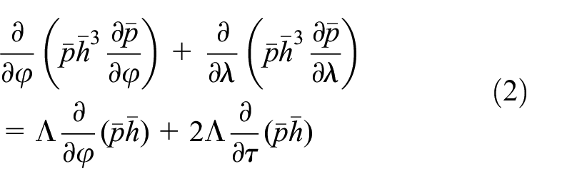
Equation (1) is an expression of the unsteady Reynolds equation. Let

where,
Once pressures of all node are determined, the load capacity of the bearing can be obtained by

Rotor dynamics equation and numerical solution process
For the symmetric rigid rotor system supported by GFB as shown in Figure 2, the dynamic model at the static equilibrium position is expressed as follows:

where,
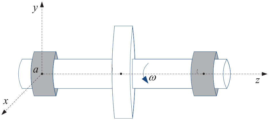
GFBs-rigid rotor system model.
In fact, the general form of equation (6) is written as

where, a represents acceleration, xc, yc are displacements of the journal from bearing center, and t denotes time.
Verlet integration algorithm is employed to construct the relationship between acceleration, velocity and displacement, as shown in equation (9), in which

Also, we can derive a formula for the displacement y that similar to equation (8). Then, the eccentricity

Trajectory method based on coupled fields
In order to understand transient behavior of the journal, the trajectory method based on coupled fields is applied. It couples gas film pressure and rotor motion. The iterative process is depicted in Figure 3, and the specific steps are listed by
(1) Given initial conditions (eccentricity and attitude angle), solving equation (4) to obtain the initial gap film pressure. Integrate the pressure to obtain the gap film resultant force, and then derive the acceleration through equation (8).
(2) The displacement and velocity of the rotor at this time are calculated by using Verlet algorithm and equation (9).
(3) The eccentricity and attitude angle of the rotor are computed by equation (10), and as the initial value for the next iteration. Repeating the above steps will get information about the shaft orbit of the rotor with time-varying.

The calculation process of trajectory method.
Calculation of dynamic coefficient
In fact, GFBs-rotor system has strong nonlinear characteristics. Usually, the higher the speed, the more significant the nonlinear phenomenon. For the case where rotor speed is small, the frequencies of input and output signals are same, which means a linear problem. Thereupon, the frequency response function method can be used to solve the dynamic coefficients. However, for the large rotor speed, the output signal will contain many components that are different from the excitation frequency. Thus, equivalence coefficient method was used to consider the nonlinear phenomenon.
Identification method of dynamic coefficients based on frequency response function
Frequency response function based on dynamic equation
The motion equation of the rotor under the excitation force is written by

where, x, y represent the displacements from static equilibrium point,
Dimensionless form the equation (10) is

where, the dimensionless quantization is perform as follows,
In the simulated excitation, harmonic excitation as input has the following expression

where,
The corresponding response, namely, rotor displacement as output is expressed as

where,
Thereupon, the frequency response function of GFBs-rotor system is described as:

where,
Frequency response function based on trajectory method
In the research, we used numerical experimentation to calculate the frequency response function. According to the coupled field model proposed previously, the displacement of the rotor can be simulated by trajectory method. And some mathematical tools such as spectral analysis and Fourier transform will be used to construct frequency response function.
The external excitations with an angular speed

Corresponding displacements are defined by
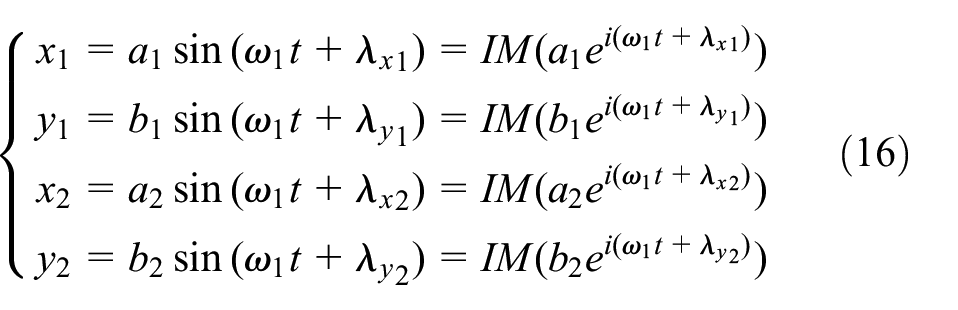
In the simulated excitation, the
The frequency response functions of numerical experimentation are defined as the followings

where,
Fast Fourier Transform (FFT) is utilized to analyze the spectrum of the displacement. In order to get analytical formula of the displacement, we rewrite the discrete displacement signals by a Fourier series as follow

where,
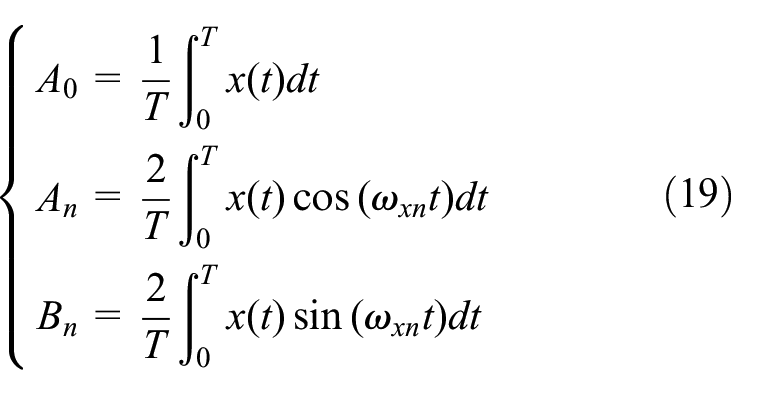
here,
Consequently,
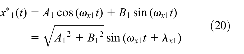
where,
Identification of dynamic coefficients
The identification of dynamic coefficients is actually a curve fitting process of two frequency response functions. The goal is that finding appropriate coefficients to get best consistency. We define an error function, and use the particle swarm optimization (PSO) algorithm to search the optimal solution (minimum value). Applying the external excitation in two directions in equation (11), there are

By substituting equation (21) into equations (12) and (13), the first two equations of equation (22) are divided by

where,
The error function G is defined by using (17) and (22)

In the PSO method, the solution to the error function is represented by a group of particles

Each particle is successively substituted into the equation (24) to obtain the error value vector.

Finding the minimum value of the error function of N particles and compare it with the next iteration. The specific process is listed as
(1) Initialize the position and velocity of the particle swarm, generate initial solution set as the current population;
(2) Calculate the fitness (error function value) of each particle in the current population;
(3) The fitness of particles is compared with each other to find the smallest value as the optimal value, record it to prepare for the next iteration;
(4) The optimal value of step 3 is compared with the optimal value of the previous iteration record, and the minimum value is selected as the global optimal value;
(5) Update the velocities and positions of the particle and return to the step 2 until the accuracy requirement is achieved (Figure 4).

PSO calculation flowchart.
Equivalence coefficient method
Under external excitation, the system response may contain multiple frequencies. The gas film force and displacement obtained through trajectory method also contain nonlinear factors. If the harmonic component in the response is too large, the equivalent coefficient method can be used to solve the dynamic characteristic coefficients. The coefficients are determined by using the data from the trajectory method, including displacement, velocity, gas foil force, and acceleration. Then the actual air foil force can be calculated by using equation (25). Although the coefficients are linear, the gas film forces calculated by equation (25) contain nonlinear factors. From this point of view, the equivalent coefficient method can consider nonlinear effects. Further, substituting the data within all-time steps in the trajectory method into equation (25) yields N equations containing eight unknowns. These equations form an overdetermined system of equations, and the eight dynamic characteristic coefficients are further identified by the nonlinear least squares method with damping. This method considers the influences of all harmonic frequencies on the coefficients, which means a nonlinear system can be equivalent to a linear system. The implementation of the equivalent coefficients method is similar to section “Frequency response function based on trajectory method,”, but only one-time excitation is required.
The motion of the rotor without mass eccentricity are written as

Where
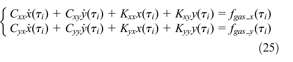
In equation (25),
The error between the equivalent gas film force and the gas film force
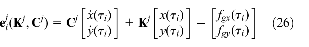
where
The overall error for the system of equations is obtained by summing the errors for each equation:
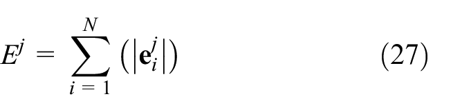
where
By constantly changing the assignments of
(1) To begin the algorithm, assign the values
(2) After completing k iterations, the current Jacobi matrix

(3) Solve the incremental equation

where
(4) If
The specific flowchart is given in Figure 5. As follows:
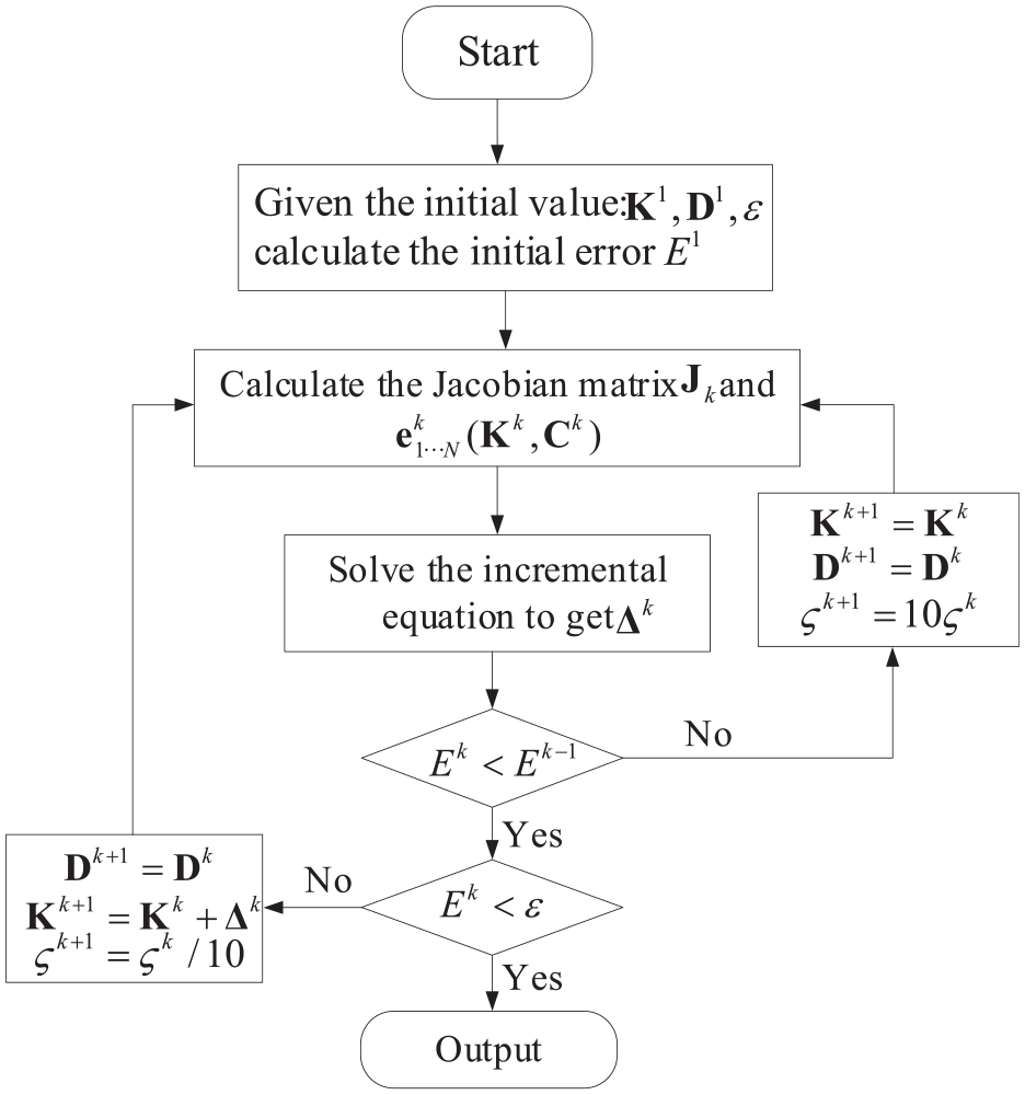
Calculation procedure diagram of algorithm.
Example and analysis
The parameters of GFBs-rotor system are shown in Table 1. Two cases with different rotor speed are considered.
The main parameters of the GFB.

where the external excitations applied in the frequency response function are represented by
Case 1: The results of linear system
In case 1, rotor speed is 30,000 rpm, and shaft orbits of numerical simulation are shown in Figure 6. For the coast down of the rotor, when discarding and considering external excitation (ignoring unbalanced mass force), the shaft orbits are shown in Figure 6(a) and (b), respectively. It shows that the shaft orbit in Figure 6(b) are larger than that of Figure 6(a) because of the centrifugal effect.

(a) Shaft orbit without unbalanced mass force and external excitation. (b) The shaft orbit without unbalanced mass force and with external excitation with
Displacements of the rotor relative to the static equilibrium point under harmonic excitation are illustrated in Figure 7. It shows that the displacements seem a harmonic vibration. The spectrum of displacements is shown in Figure 8. Among these frequency components, the amplitude of 500 Hz (equal to the excitation frequency) is maximum. Meanwhile, there are other components, such as 79.5 Hz, 155.883 Hz, 182.167 Hz, and their amplitudes are very small. In summary, the case 1 seems a linear problem.

(a) Displacement comparison in x direction with external excitation. (b) Displacement comparison in y direction with external excitation.
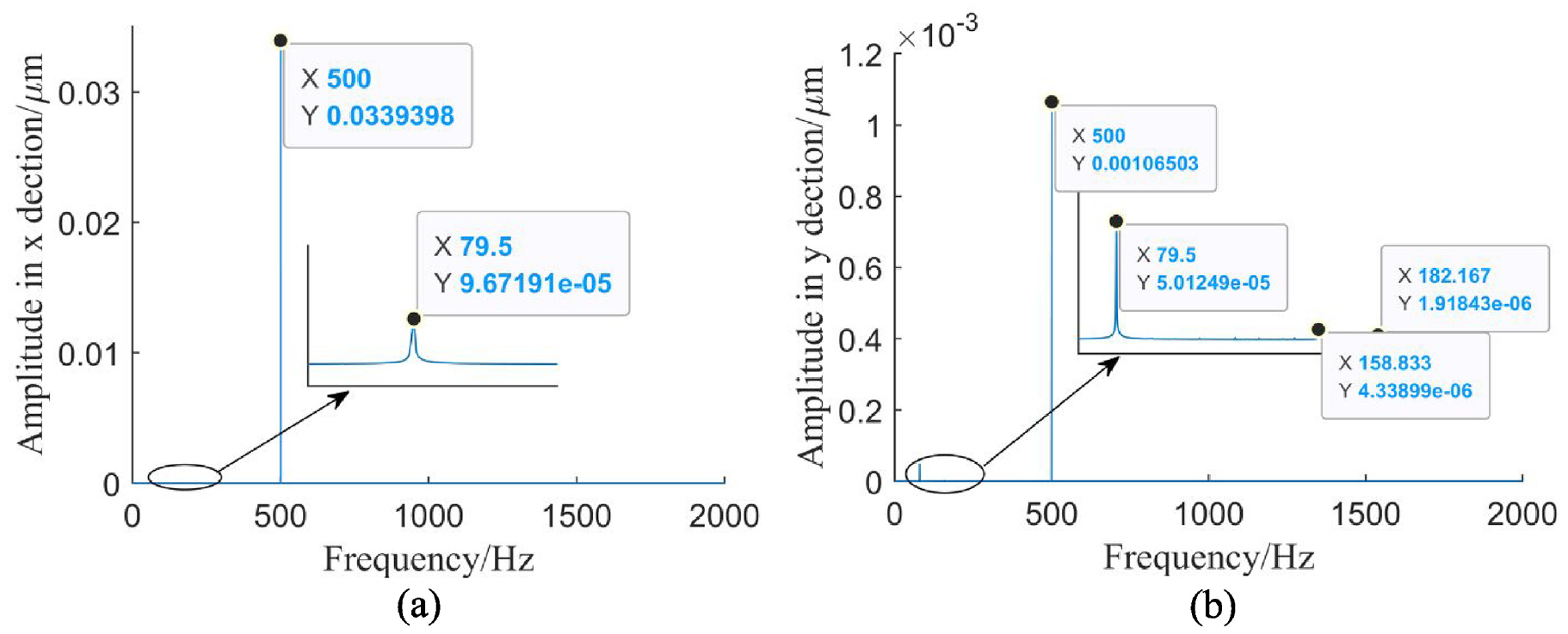
(a) x-direction displacement spectrum analysis. (b) y-direction displacement spectrum analysis.
Using equation (21), the 500 Hz component

(a) The displacement in the x direction and the phase difference of the external excitation. (b) The displacement in the y direction and the phase difference of the external excitation.
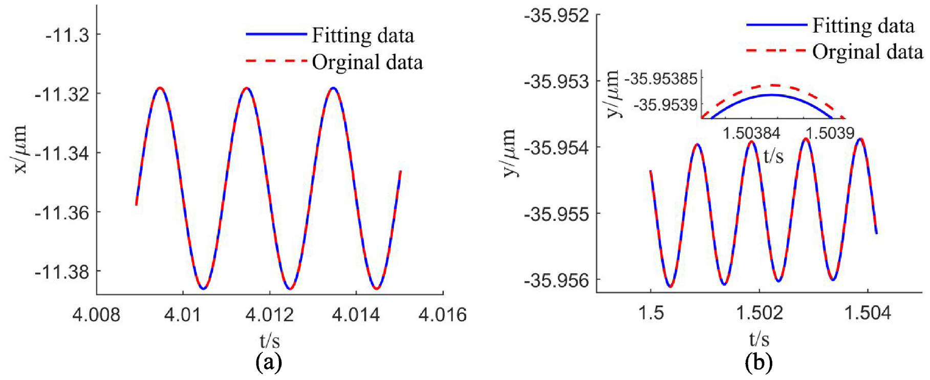
(a) Comparison of the x-direction reconstruction displacement and the original displacement. (b) Comparison of the x-direction reconstruction displacement and the original displacement.
The dynamic coefficients identified by the frequency response function are compared with the perturbation method, as shown in Table 2. With the results of the perturbation method as a reference benchmark, the conclusion can be summarized as follows.
Dynamic coefficients of GFB with 30,000 rpm.

(1) The average main stiffness coefficients
The reasons for the difference between the above two methods (perturbation method, frequency response function method) are as follows. The perturbation method is based on solving the dynamic Reynolds equation, ignoring the higher order terms of the nonlinear gas film force. But frequency response function method applies the coupled fields, and can consider more practical gas film force and rotor motion. In addition, the perturbation method can only consider a single whirl ratio, which is man-made assumptions and lacks practicality. However, the frequency response function method considers the actual whirl frequency. The frequency response function is fitted by PSO algorithm, and the dynamic coefficient is finally identified.
Case 2: The results of nonlinear system
In case 2, rotor speed is set as 60,000 rpm, and shaft orbits of numerical simulation are shown in Figure 11.
For the coast down of the rotor, when discarding and considering external excitation (ignoring unbalanced mass force), the shaft orbits are shown in Figure 11(a) and (b), respectively. Figure 11(a) illustrates the rotor has an elliptic shaft orbit for the absence of external excitation. However, under the effect of external excitation, the rotor whirls irregularly near the static equilibrium position, as shown in Figure 11(b). Compared with Figures 6 and 11, the form of rotor whirling will change with the rotation speed. The curves of the steady-state displacement over time are shown in Figure 12, and it can be observed that the effect of the external excitation on the displacement is very significant. To investigate the effect, the spectrum of rotor displacement under external excitation is plotted, as shown in Figure 13. For the case 1, the external excitation frequency (500 Hz) is main frequency as shown in Figure 8. Nevertheless, as to the case 2, the whirl frequency (89 Hz) is the main frequency as shown in Figure 13. It can be concluded from the results that the amplitude of the whirl frequency component increases with the rise of the speed, which makes the system tend to unstability. Figure 14 shows that the reconstructed displacement exhibits good consistency with the original displacement.
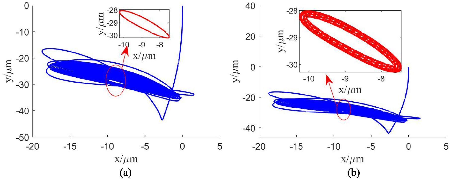
(a) Shaft orbit without unbalanced mass force and external excitation. (b) The shaft orbit without unbalanced mass force and with external excitation with 60,000 rpm.

(a) The time domain diagram of x-displacement. (b) The time domain diagram of y-displacement.

(a) Spectrum of x-direction displacement. (b) Spectrum of y-direction displacement.

(a) Comparison of the x-direction reconstruction displacement and the original displacement. (b) Comparison of the y-direction reconstruction displacement and the original displacement.
The calculation results of the perturbation method and the equivalence coefficient method are shown in Table 3. With the results of the perturbation method as a reference benchmark, the conclusion can be summarized as follows.
Dynamic coefficients of GFB with 60,000 rpm.

The stiffness coefficients obtained by both methods, namely, the equivalence coefficient method and the perturbation method, are relatively close. With the results of the perturbation method as a reference benchmark, the difference between Kxx and Kyy are 4.7% and 16%, respectively. The damping coefficients in the x and y directions are quite different, and the former is about seven times and two times of the latter, respectively.
The equivalent coefficient method includes all whirl effects, in other words, the nonlinear force at a certain rotational speed is forcibly expressed as an equivalent by linear coefficients. In a sense, although the obtained dynamic stiffness and damping coefficients are equivalent linearization coefficients, they also can reflect nonlinearity.
Modal and stability analysis of rotor
The stability of a gas foil bearing rotor system depends on the dynamic characteristic coefficients. Assuming that the stiffness is much greater than the damping and that the damping is negligible, the dynamic equations of the rotor system supported by the gas bearing can be expressed as follows:

The rotor undergoes simple harmonic motion, as described by the characteristic equation:

If the mass matrix
Taking 30,000 rpm as an example, the dynamic characteristic coefficients can be substituted into (29) to obtain eight characteristic roots:
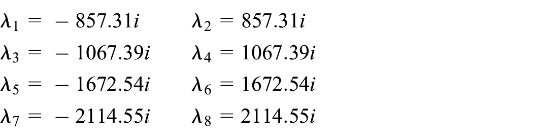
By substituting the characteristic roots obtained into equation (28), four feature vectors can be derived:

The natural frequency calculated in finite elements is (Table 4):
Modal comparison between analytical method and finite element method.

Figures 15(a) to (d) show the rigid body modes of the rotor, while Figures 15(e) and (f) show the bending modes. The rotor experiences parallel vortex (resonance) when the external excitation frequency reaches 136.44 Hz and 169.88 Hz, and conical vortex (resonance) when the external excitation frequency reaches 266.19 Hz and 336.54 Hz.

Rotor mode at 30,000 rpm.
Conclusions
Based on the trajectory method, the fluid-solid coupling dynamic model of GFBs-rotor system is established, and the transient trajectory of the rotor is solved. The dynamic coefficients identification method for simulated excitation is proposed. The following conclusions are drawn:
(1) The average main stiffness coefficients
(2) The stiffness coefficients obtained by both methods, namely, the equivalence coefficient method and the perturbation method, are relatively close. With the results of the perturbation method as a reference benchmark, the difference between Kxx and Kyy are 4.7% and 16%, respectively. The damping coefficients in the x and y directions are quite different, and the former is about seven times and two times of the latter, respectively.
(3) The equivalent coefficient method includes all whirl effects, in other words, the nonlinear force at a certain rotational speed is forcibly expressed as an equivalent by linear coefficients. In a sense, although the obtained dynamic stiffness and damping coefficients are equivalent linearization coefficients, they also can reflect nonlinearity.
The two methods proposed in this paper are to use the numerical simulation results of the coupled field to identify the dynamic parameters, so it is closer to the actual situation than the perturbation method.
Footnotes
Handling Editor: Sharmili Pandian
Declaration of conflicting interests
The author(s) declared no potential conflicts of interest with respect to the research, authorship, and/or publication of this article.
Funding
The author(s) disclosed receipt of the following financial support for the research, authorship, and/or publication of this article: This work is supported by the National Natural Science Foundation of China (No. 51705413, 52275271, 11972282, 6110119004) and the Shaanxi Natural Science Foundation Research Plan (No. 2022JM-194).